Spatial and Temporal Variability in Bioswale Infiltration Rate Observed during Full-Scale Infiltration Tests: Case Study in Riga Latvia

Abstract

Urban nature-based solutions (NBSs) are widely implemented to collect, store, and infiltrate stormwater. This study addressed infiltration rate as a measure of the performance of bioretention solutions. Quick scan research was conducted, starting with mapping over 25 locations of implemented green infrastructure in Riga, Latvia. Basic information, such as location, characteristics, as well as photos and videos, has been uploaded to the open-source database ClimateScan. From this, eight bioswales installed in the period 2017–2022 were selected for hydraulic testing, measuring the infiltration capacity of bio-retention solutions. The results show a high temporal and spatial variation of infiltration rate for the bioswales, even those developed with similar designs: 0.1 to 7.7 m/d, mean 2.0 m/d, coefficient of variation 1.0. The infiltration capacity decreased after saturation: a 30% to 58% decrease in infiltration rate after refilling storage volume. The variation in infiltration rate as well as infiltration rate decrease on saturation is similar to other full-scale studies done internationally. The infiltration rate of most bioswales falls within the range specified by international guidelines, all swales empty within 48 h. Most bioswales empty several times within one day, questioning the effectiveness of water retention and water availability for dry periods. The results are of importance for stakeholders involved in the implementation of NBS and will be used to set up Latvian guidelines for design, construction, and maintenance.

1. Introduction

Climate change (with higher temperatures and high intensive rainfall) and urbanisation (with an increasing impervious land cover) affect the urban water balance, resulting in flooding, heat stress, and droughts. According to the Intergovernmental Panel on Climate Change, the frequency and intensity of heavy precipitation have likely increased globally and very likely increased in Europe since the 1950s. Both global and regional (convection permitting) climate models project with high confidence an increase in extreme precipitation, and, by direct association, pluvial flooding in the Northern and Central European regions, where Latvia belongs [1]. Apart from the extreme precipitation enhanced by climate change, urban pluvial floods are attributed to urbanisation, increased sealing, and decreased infiltration [2,3,4,5]. Alongside increased extreme precipitation and pluvial flooding, there have been global increases in the intensity and duration of heat waves [1]. This, combined with a decrease in green areas because of urbanization, drives a more frequent prevalence of heat stress and drought conditions in cities [1,6,7].

As a response to the multiple challenges presented by urbanisation and climate change, nature-based solutions (NBSs), also called Sustainable Urban Drainage Systems (SuDSs), blue and green infrastructure (BGI), and sponge city approaches are being deployed actively throughout the world [8,9,10,11,12,13]. Further in the article, we use the term ‘Nature-based solutions’ (NBSs), which is defined as “solutions that are inspired and supported by nature, which are cost-effective, simultaneously provide environmental, social and economic benefits and help build resilience” [14]. Examples of NBSs for urban stormwater management include bioretention features like rain gardens or bioswales, permeable pavements, green roofs and green walls, artificial wetlands, sedimentation ponds, and others [15]. These techniques have multiple benefits in the broad categories of hydraulic control and flood avoidance/reduction, water treatment, biodiversity enhancement, microclimate improvement, amenity, and recreation, which are often conflicting and thus careful planning is important considering the specific context [14,16,17].

Some of the most popular NBs, both globally and in Latvia, are bioretention features, which are also known as rain gardens, swales, bioswales, and biofilters. Bioretention systems are constructed techniques comprising surface depression for temporary storage of runoff and constructed soil layers typically designed for quick infiltration as well as a variety of plants. Depending on the site and design requirements, bioretention features may contain an underdrain/overflow connected to a stormwater sewer as well as internal water storage [18]. Bioretention features such as bioswales are designed to reduce the peak flow rate and volume of runoff through water attenuation and infiltration and have been used for decades globally to provide infrastructure conveyance and water quality treatment [19].

Bioretention systems ensure a significant reduction in peak runoff, delivering a 40–99% average reduction, as well as the total volume of runoff, averaging a 58% reduction. However, there is still a deficit of information on the performance of real-life systems due to the difficulty in long-term monitoring of such systems [20]. Other research needs include research on optimal media composition, the role and selection of plants for optimal bioretention performance, the study of internal water storage and the outlet section, and long-term research studies that provide calibration data for the models prepared to predict long-term performance [18,21].

Infiltration capacity is an important factor influencing the performance of bioretention systems [18,22]. Many international guidelines suggest an infiltration rate of 100–300 mm/h [23] or an emptying time within 24–48 h [24,25]. Addressing the need to provide data on the infiltration rate in real-life systems, several studies have undertaken full-scale infiltration tests in bioretention features, establishing a high degree of spatial and temporal variability in the infiltration rate [23,24,26].

As a part of the solution to make Baltic States climate-adaptive, the first NBSs have been implemented that enable rainfall infiltration and the evapotranspiration of stored water to mitigate the effects of drought and heat stress, but also intensive rainfall events causing floodings. Examples of green infrastructure implemented in recent years include permeable pavements, artificial wetlands, green roofs and green walls, and most importantly, bioretention systems [27].

The methodology and regulation basis for implementing sustainable urban drainage solutions is still developing in Latvia. There are local guidelines on the design of sustainable urban drainage techniques by an NGO, Cleantech Latvia [28], which provide typical sections of bioretention features; however, there are no guidelines on infiltration rates or emptying times. Very often infiltration rates are not taken into account while designing at all, considering only surface storage for dealing with the volume of surface runoff.

Therefore, the study aims to determine the infiltration rate in the recently created bioretention solutions in the capital of Latvia, Riga, and compare it to similar studies conducted internationally as well as design guidelines. The study both addresses the international need for research on implemented bioretention solutions as well as to build local knowledge on water-balance-optimal bioswale design. To that end, full-scale infiltration tests were performed in July and October 2023 in eight bioswales installed in the period 2017–2022 in Riga, Latvia.

2. Materials and Methods

2.1. Study Site Selection

The study sites were selected using ClimateScan—an open-source, interactive web-based map application for international knowledge exchange on ‘blue-green’ projects around the globe [29,30]. The platform features more than 14,000 climate adaptation solutions around the world including more than 6000 NBS locations. The database contains basic information, such as location, characteristics, as well as photos and videos, and for the featured projects—links to research performed on specific locations. It is the most comprehensive source of information about NBSs in Latvia, featuring over 70 locations related to climate adaptation (e.g., green roofs, constructed wetlands, and floating structures) with over 25 locations with biofiltration, such as bioswales, implemented in Riga (see Figure 1a). The projects in Latvia have been mapped since 2018 through stakeholder involvement events called climate cafes and individually by users and experts in the field [27]. Figure 1 shows location sites mapped in Riga in the platform as well as the locations of the study sites.

The three locations were selected for research based on the year of construction (not older than 10 years), the presence of detailed design documentation and known rationale for the design choices, as well as access to the sites for testing purposes.

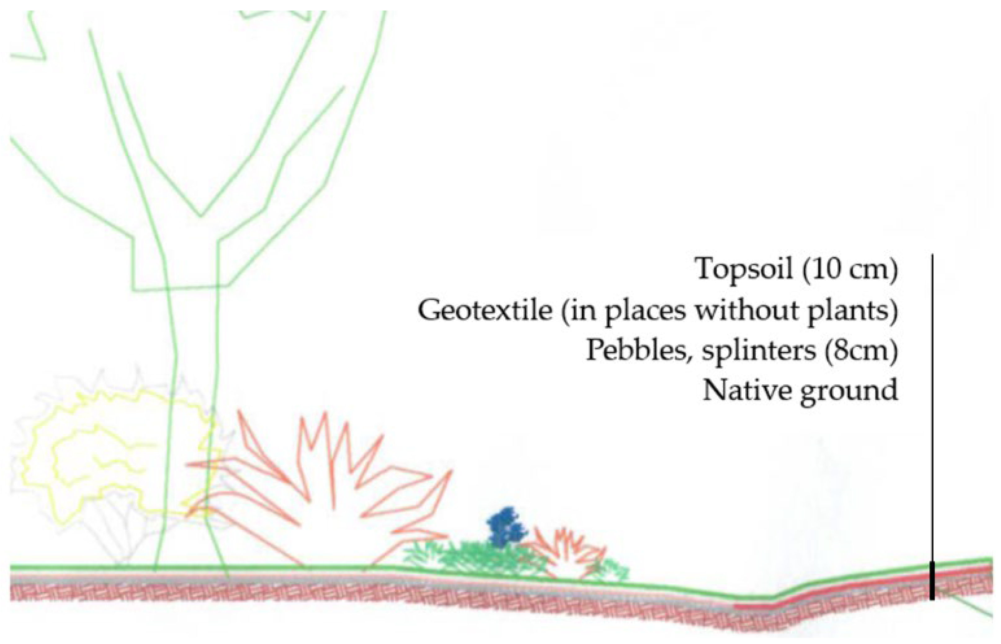
2.2. Study Site Description

Sites 1 and 2 have been developed on former industrial properties, whereas Site 3 is a greenfield site. Sites 1 and 2 are residential developments constructed in 2020–2021 by the residential real estate developer Bonava. Site 3 is a parking lot of a shopping centre SPICE Home with two symmetrical bioswales, developed in 2017. See Figure 2 for bioswale locations within the study sites.

The bioswales in Sites 1 and 2 are implemented with the same design, with the only exception being the presence of underdrains and overflow at Site 2. Such difference is due to the fact that conditions on Site 1 (low groundwater level, well-draining surrounding soil on the one hand, and the absence of connection to the municipal storm sewer, on the other hand) have resulted in a completely decentralised stormwater management system, with runoff leaving the site only through exfiltration and evapotranspiration. In Site 2, on the other hand, a fully decentralised system was not possible due to high groundwater levels, so a restricted connection to the municipal system is provided.

Bioswales 1–6 have a storage depth up to 30–50 cm with overflow at typically 15–30 cm above the bottom of the swales. Bioswales 1–4 (Site 1) are implemented without underdrains and thus lose water only through exfiltration and evapotranspiration; Bioswales 1–2 and 3–4 are connected through an overflow pipe. Bioswales 5–6 are equipped with underdrains below the filter media, losing water additionally through drainage. In these swales, there is also an overflow connection to the underdrain.

The design choices for Bioswales 7 and 8 at Site 3 are explained by the high groundwater level. The bioswales have a depth of up to 45 cm and overflow pipe 10 cm above the bottom of the swales, connected to the municipal storm sewer.

All bioswales have perennial plants in the zone below overflow and trees and shrubs in the zone above overflow, based on the study of plants suitable for similar systems internationally as well as local guidelines [28]. The exception is Swale 6, which has grass only, and the reason for this design choice is unknown.

The photos of the bioswales are shown in Figure 3.

Table 1. Bioswale details.

Swale #	Area, m2	Catchment Area (Excl. Swale), m2	Catchment Surfaces	Outflow via	Surrounding Soil Conditions	Groundwater Depth below Swale Bottom, m *	Plants
Swale 1	95	604	Building roof, parking lot, sidewalks	Exfiltration, overflow to Swale 2	Artificial soil: sand with construction rubble and organics	1.3	Perennial plants: Eupatorium fistulosum, Molinia arundincea, Miscanthus sinensis, Physostegia virginiana Trees and shrubs: Salix purpurea, Salix fragilis, Betula utilis var. jacquemontii
Swale 2	88	656	Parking lot, sidewalks	Exfiltration, overflow to Swale 1		1.7
Swale 3	140	798	Parking lot, sidewalks	Exfiltration, overflow to Swale 4	Downstream: Artificial soil: sand with construction rubble and organics, sandy peat with construction rubble Upstream: Artificial soil: sand with construction rubble and organics, degraded peat and sandy peat	1.1
Swale 4	88	379	Parking lot, sidewalks	Exfiltration, overflow to Swale 3	Artificial soil: sand with construction rubble and organics, degraded peat and sandy peat	1.3
Swale 5	175	1241	Parking lot, sidewalks, playground	Exfiltration, underdrain, overflow to underdrain, located at the edge of the swale	Artificial soil: sand with construction rubble and organics, coarse sand	0.7	Perennial plants: Carex elata, Eupatorium fistulosum, Iris pseudacorus, Iris sibirica, Lysimachia punctata, Miscanthus sinensis, Molinia arundincea, Nepeta mussinii Trees and shrubs: Salix fragilis Betula utilis var. jacquemontii
Swale 6	53	600	Parking lot, sidewalks	Exfiltration, underdrain, overflow to underdrain, located for the entire length of the swale
Swale 7	358	2355	Parking lot	Exfiltration, overflow to municipal sewer	Greenfield: sand, dusty, dense, saturated with water, yellow and pale yellow	0.6	Perennial plants: Miscanthus sinensis, Miscanthus purpurascens, Iris sibirica Trees and shrubs: Coloneaster dammer, Salix purpurea, Salix repens, Quercus robur, Physocarpus opulifolius
Swale 8	352	2659	Parking lot	Exfiltration, overflow to municipal sewer

* Based on geology surveys during construction stage, except for Swales 5–6, which are based on groundwater level sensor in Swale 5.

shows details of the bioswales.

Figure 4 and Figure 5 show the typical cross-section and filter media composition of Bioswales 1–6 and 7–8 respectively, as per the design documentation.

2.3. Full-Scale Infiltration Testing

Full-scale infiltration testing has been introduced as a way to overcome high variability in point infiltration capacity measurements. Full-scale infiltration tests have been successfully used in bioretention features like swales as well as permeable pavements [31,32].

In this study, the bioswales were filled up repeatedly up to the point of overflow (overflow structures were closed off with plastic sheets and duct tape) through a firefighting hose, connected to the street fire taps. Then, the drop in water level to the empty or nearly empty level was registered with pressure sensor data loggers [33,34]. Wireless, self-logging pressure transducer loggers were used in the study as the primary method of measuring and recording the reduction in water levels over time. The loggers were individually factory-calibrated and tested to ensure that at least 68% of measurements during the calibration check were within the stated typical accuracy. The transducers continuously monitored the static water pressures in the bioswales, logging the data in internal memory.

Figure 6 illustrates the performance of the infiltration tests in Bioswale 2 and Bioswale 8.

To back up the data, measurements were performed with several sensors as well as supplemented with visual observations using a ruler and time-lapse photography. An infiltration test at one site was carried out for one full day, filling up the swales repeatedly when they were empty or half empty. Data loggers were left in the swales for a certain amount of time to register the emptying of the swales after the end of the day, where possible. Infiltration tests were performed on 13 July 2023 in Bioswales 1–4, on 14 July 2023 in Bioswales 5–6, and then repeatedly on 16 October in Bioswales 1–4, as well as additionally on 17 October in Bioswales 7–8.

Table 2. Conditions before and during the infiltration tests.

Swale and Date	Number of Tests	Sensors Used	Sensor Accuracy	Logging Frequency	Measurement Verification	Presence during the Test	Environmental Conditions before and during the Test
Swale 1—13 July 2023	2	2 TD-diver loggers	±0.5 cm H2O	5 s	2 sensors	Two people supervised the test for the entire duration of test 1 and halfway through test 2, sensors were extracted in the evening	Abnormally dry months of April–June 2023 in Riga: cumulative precipitation 37.9 mm compared to the climatic norm of 150.7 mm over the three months, in the first 10 days of July the precipitation amount was lower by 28% compared to the norm, the average temperature in April was higher by 1.4 °C, in May by 0.2 °C, in June by 1.6 °C compared to the climatic norm. Last rainfall 7 days before the test with a depth of 3.8 mm
Swale 2—13 July 2023	3	1 CTD-diver logger for tests 1–3 and 1 TD-diver logger for tests 1–2	±0.5 cm H2O	5 s	2 sensors, time-lapse photos	Two people supervised the test for the entire duration of tests 1 and 2 and 75% of test 3, sensors were extracted in the evening
Swale 3—13 July 2023	1	CTD-diver logger in the downstream part, TD-diver logger in the upstream part	CTD-diver: ±2.5 cm H2O TD-diver: ±0.5 cm H2O	1 s in the downstream part 0.5 s in the upstream part	2 sensors	Two people supervised the test for 58% of the test duration, the sensors were extracted in the evening
Swale 4—13–14 July 2023	1	TD-diver logger	±0.5 cm H2O	5 s	Visual inspection with a ruler	Two people supervised the test for 15% of the test duration, the site was inspected in the evening, and the sensor was extracted the next morning
Swale 5—14 July 2023	2	2 TD-diver loggers	±0.5 cm H2O	5 s	2 sensors, time-lapse photos	Two people supervised the test for the entire duration of test 1 and 75% of test 2, the sensors were extracted the next morning	Same conditions as Swales 1–4. Rainfall of 3 mm during test 2
Swale 6—14 July 2023	4	2 TD-diver loggers	±0.5 cm H2O	5 s	2 sensors	Two people supervised the test for the entire duration of all tests	Same conditions as Swales 1–4
Swale 1—16 October	2	TD-diver logger	±0.5 cm H2O	5 s	Visual inspection with a ruler	Two people supervised the test for the entire duration of test 1 and halfway through test 2, sensors extracted in the evening	Abnormally wet months of July and August: 264.6 mm of rainfall compared to the norm of 158.2 mm. Abnormally dry September: 36.2 mm of rainfall compared to the norm of 66 mm. In the first 10 days of October, the precipitation amount exceeded the norm by 100% and in the second 10 days by 50%. Last rainfall: 5.8 mm the previous day. Rainfall of 1.2 mm during the test day
Swale 2—16 October	3	TD-diver logger	±0.5 cm H2O	5 s	Time-lapse photos	Two people supervised the test for the entire duration of test 1 and 2 and 75% of test 3, the sensor extracted in the evening
Swale 3—16 October	1	TD-diver logger	±0.5 cm H2O	5 s	Visual inspection with a ruler	Two people supervised the test for 75% of the test duration, the sensor was extracted in the evening
Swale 4—16–18 October	1	TD-diver logger	±0.5 cm H2O	5 s	Visual inspection with a ruler	Two people supervised the test for 25% of the test duration, the sensor was extracted in the evening
Swale 7—17–18 October	2	TD-diver logger	±0.5 cm H2O	5 s	Visual inspection with a ruler	Two people supervised the test for the first 2 h, the site was inspected in the evening, and on October 18, the sensor was extracted in the morning of October 19	Same conditions as Swales 1–4. Rainfall of 13.2 mm between the tests
Swale 8—17–18 October	2	2 TD-diver loggers	±0.5 cm H2O	5 s	2 sensors

summarises the conditions of infiltration tests performed in different swales in July and October 2023.

2.4. Data Processing

The raw data obtained during the tests comprised uncompensated pressure data in cm H₂O. Pressure sensor readings were compensated with the atmospheric pressure data to calculate the water level above the sensor. Time series of specific emptying sequences (water level drop) were extracted from subsequent tests and analysed using linear regression. The resulting slope of the linear regression was used to calculate the infiltration rate in m/d. The detailed data processing pipeline is shown in Figure 7.

Alternative data processing methods include calculating the infiltration rate based on the difference in the full and empty level (absolute difference) divided by time or calculating the infiltration rate as the effective storage volume of water in the system between 75% and 25% effective storage depth divided by the product of the internal surface area of the system up to 50% effective storage depth and including the base area and the time for the water level to fall from 75% to 25% effective storage depth [35]. Although the latter method may be more precise in calculating saturated hydraulic conductivity, the method used in this study was chosen to facilitate comparing the results of the study with other international studies conducted on full-scale infiltration testing.

3. Results

3.1. Results of Individual Infiltration Tests

Figure 8 shows the infiltration rate calculation for Bioswales 1–4, placed in the same location (Site 1), for infiltration tests on July 13–14 (panels a, c, e, g) and 16–17 October (panels b, d, f, h). The panels of the figure show the water level changes in respective swales as well as linear regression trendlines derived to calculate the infiltration rate, with coefficient a (slope) denoting infiltration rate in cm per hour.

The figures show the variability in infiltration rate between the two testing dates, between the consecutive infiltration tests of the same swale as a variation in infiltration rate between the swales, constructed with the same design.

Moreover, the results obtained for Swale 3 indicate infiltration rate differences in the same swale (Figure 9). The sensor placed in the downstream part of the swale (Figure 9a) showed not only a higher infiltration rate for the entire test compared to the sensor placed in the upstream part of the swale (Figure 9b), but also a higher infiltration rate in the second half of the emptying time, compared to the first half. This can be explained by the fact that the swale is the longest in the site, having a non-uniform slope and micro-pools, and when the water level in the upstream part of the swale dropped below 10 cm (approximately 3.5 h into the infiltration test), the downstream part of the swale became hydrologically isolated from the upstream part. Figure 9a shows the depth measured by the sensor downstream of the swale, whereas the sensor placed upstream of the swale (closer to swale 4, which had the lowest infiltration rate) showed a lower infiltration rate, as seen in Figure 9b.

Similar variability is seen in Bioswales 5–6, placed in different locations but delivered with a similar design, the only difference being an underdrain below constructive layers of the swale. See Figure 10 for the results of the infiltration tests, which were performed once in July 2023.

At Site 3, infiltration tests were carried out on October 17–19. The results of the full-scale infiltration testing are shown in Figure 11. The gap between the test 1 and test 2 time series in the charts is a rain event that happened during the infiltration test; thus, a slight increase in water level can be seen in the charts.

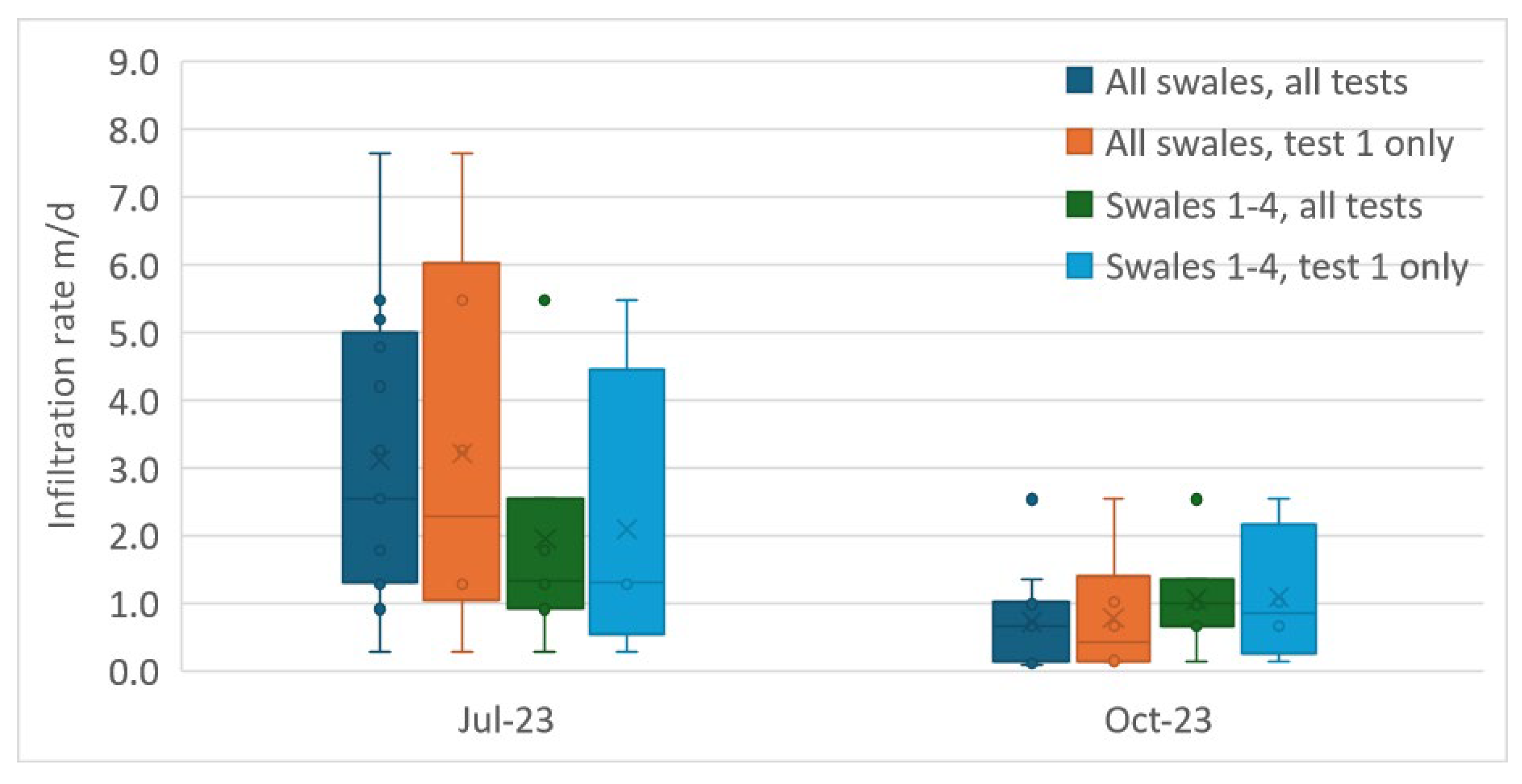
3.2. Summary of the Results

The results of all infiltration tests are summarized in

Table 3. Infiltration test results summary—infiltration rate in meters per day.

	13–14 July 2023
Test #	Swale1	Swale2	Swale3	Swale4	Swale5	Swale6
Test 1	1.28	5.48	1.33	0.29	3.26	7.65
Test 2	0.92	2.55			1.84	5.20
Test 3		1.78				4.66
Test 4						4.20
	16–19 October 2023
Test #	Swale1	Swale2	Swale3	Swale4	Swale7	Swale8
Test 1	1.03	2.54	0.67	0.14	0.16	0.18
Test 2	0.69	1.35			0.09	0.11
Test 3		0.99

. The infiltration rate in meters per day is shown, calculated from the linear regression trendline slope coefficient of the water depth time series. For the swales where two sensors were installed (Swales 1, 2, 3, 5, and 6 in July 2023 and Swale 8 in October 2023), the average result of the two sensors is shown in the table.

Figure 12 visualises the results of the infiltration tests.

Table 4. Infiltration test results summary—infiltration rate in meters per day.

Parameter	All Swales and All Tests	All swales, Test 1 Only	July 2023				October 2023
			All Swales, All Tests	All Swales, Test 1 Only	Swales 1–4, All Tests	Swales 1–4, Test 1 Only	All Swales, All Tests	All Swales, Test 1 Only	Swales 1–4, All Tests	Swales 1–4, Test 1 Only
n	24	12	13	6	7	4	11	6	7	4
Minimum (m/d)	0.09	0.14	0.29	0.29	0.29	0.29	0.09	0.14	0.14	0.14
Maximum (m/d)	7.65	7.65	7.65	7.65	5.48	5.48	2.54	2.54	2.54	2.54
Mean (m/d)	2.02	2.00	3.12	3.22	1.95	2.10	0.72	0.78	1.06	1.09
Median (m/d)	1.31	1.16	2.55	2.29	1.33	1.31	0.67	0.43	0.99	0.85
Standard deviation (m/d)	2.02	2.29	2.10	2.60	1.58	2.00	0.71	0.85	0.70	0.89
Coefficient of variation	1.00	1.14	0.67	0.81	0.81	0.95	0.99	1.08	0.66	0.82

provides a statistical summary of the infiltration test results, whereas Figure 13 visualises the results in a box and whisker plot.

The results show great variability in the infiltration rate in the bioswales, with the coefficient of variation (CV, which is calculated as the standard deviation divided by the mean) being 1.00 for all of the tests performed both in July and October 2023. The variation decreases with consecutive tests.

3.3. Result Interpretation

Swales 1–4, located at the same site and designed for infiltration, showed a more than 10-fold variability in the first test in July 2023, when the filter media was least saturated. The infiltration rates are highest in Swale 2, near which the groundwater table was lower compared to the other swales, as per the geology survey performed before the construction. Considering the proximity of the swales, such differences in groundwater level can be explained by the high heterogeneity of surrounding soil conditions due to previous development at the site.

Another factor possibly explaining the much higher infiltration rate in Swale 2, compared to other swales in Site 1, is the observed preferential flow in the upper soil layer, see Figure 14a.

Notable is the presence of degraded peat and sandy peat in geology study samples near Swales 3 and 4, which had lower infiltration rates. In the upstream of Swale 3, where the infiltration rate was lower, compared to the downstream part, the geology survey indicated the presence of a continuous degraded peat layer, compared to the downstream of the swale, where peat is just one of the components of artificial soil layer. Degraded peat is known to have low hydraulic conductivity and the ability to create waterlogged areas [36].

At Site 2, a more than two-fold difference is observed in infiltration rate in Swales 5 and 6, placed at the same location and built with nearly the same design. The differences between the swales are the absence of perennial plants in Swale 6, compared to Swale 5, as well as the underdrain, which is located on the edge of Swale 5 but runs for the entire length of Swale 6. Like in Swale 2 at Site 1, preferential flow was observed in Swale 6 (Figure 14b). Interestingly, Swale 2 at Site 1, not equipped with an underdrain, showed a comparable infiltration rate to the swales at Site 2, equipped with an underdrain. This probably can be explained by the preferential flow in Swale 2, discussed above.

The technical design for Swales 1–6 specified an infiltration rate of 2–3 m/d for the upper soil layer, which was achieved in Swales 2, 5, and 6 and not achieved in Swales 1, 3, and 4. This most probably can be attributed to the surrounding soil conditions, as in the full-scale test water fills the available pore space of the filter media relatively quickly and the surrounding soil becomes the limiting factor.

Table 5. Decrease in infiltration rate in the subsequent tests.

	13–14 July 2023
Test #	Swale1	Swale2	Swale3	Swale4
Test 2	−29%	−53%	−44%	−32%
Test 3		−30%		−8%
Test 4				−12%
	16–19 October 2023
Test #	Swale1	Swale2	Swale7	Swale8
Test 2	−33%	−47%	−44%	−39%
Test 3		−27%

shows a calculated decrease in infiltration rate in subsequent tests.

It should be noted that the differences between the infiltration rate decreases between the tests are much smaller compared to the differences between the infiltration rates in the different swales. For example, for Swales 1, 2, 5, and 6, built with a similar design and for which several infiltration tests were carried out on 13–14 July, the coefficient of variation (the ratio of the standard deviation to the mean) of the infiltration rate during the first infiltration test is 0.62, whereas the coefficient of variation of the decrease in infiltration rate in subsequent tests is 0.29.

At Site 1 (Swales 1–4), where infiltration tests were performed both in July, after a long dry period, and in October, after a long period of rainfall, a decrease in infiltration rate of more than 50% was observed—see

Table 6. Decrease in infiltration rate measured in Site 1 between July and October 23.

Test #	Swale1	Swale2	Swale3	Swale4
Test 1	−19%	−55%	−58%	−53%
Test 2	−25%	−46%
Test 3		−45%

for comparison.

In all swales but Swale 1, the infiltration rate decreased by more than half, which can be explained by soil saturation due to a long rain period before infiltration tests. Volumetric soil moisture content, measured in Swale 1 with soil moisture sensors 15, 30 and 45 cm below the bottom of the swale, was, respectively, 0.31, 0.14, and 0.28 cm³ cm⁻³ before the test on July 13 and 0.37, 0.36, and 0.38 cm³ cm⁻³ before the test on 16 October, showing full saturation after a long rainfall in the autumn.

Notable is the smaller decrease in infiltration rate for Swale 1, which needs to be further investigated. A possible reason could be preferential flow to the underground cavities formed by construction rubble below the swale constructive layers through groundwater and surface water level observation borehole in the swale. This is indirectly corroborated by the soil moisture data and water depth data in the borehole during infiltration tests and rain events, not covered by this paper.

The bioswales at Site 3, where infiltration testing was performed on 17–19 October, are different in design from Sites 1 and 2 in that they are not mainly designed for infiltration but rather for water attenuation and limited discharge into the storm sewer, although infiltration is allowed through a non-lined bottom. The lower infiltration rate in these swales could be explained by the high groundwater table as well as soil saturation before the test after the long rainfall. Another possible reason could be the longer time in operation and resulting clogging of the bioretention system.

3.4. Comparison with Other Full-Scale Test Studies

The obtained results on the high temporal and spatial variability in bioswales are comparable with other full-scale infiltration test studies carried out internationally [23,24,26,37]. In these studies, the number of repeated tests performed in the bioretention features differ greatly; for example, in the study carried out in Dalfsen, the Netherlands [24], the swales were filled up and emptied up to five times, whereas the swales studied in Bergen, Norway [23] were emptied only once and filled only once. Therefore, in the case that several subsequent infiltration tests were performed in a study, like Swales 1, 2, 5, and 6 in July 2023 and Swales 1, 2, 7, and 8 in October 2023 in this study, only the results of the first infiltration tests are used in the analysis. The infiltration test comparison results are shown in

Table 7. Full-scale infiltration test results compared to other international studies of full-scale infiltration tests in bioretention features (bioswales, rain gardens, etc.).

Study	n	Minimum (m/d)	Maximum (m/d)	Mean (m/d)	Median (m/d)	Standard Deviation (m/d)	Coefficient of Variation
Present study—July (dry period)	6	0.29	7.65	3.22	2.29	2.60	0.81
Present study—October (wet period) *	6	0.14	2.54	0.78	0.43	0.85	1.08
Dalfsen, NL—drought [24]	3	3.10	8.20	5.17	4.20	2.19	0.42
Dalfsen, NL—normal conditions [24]	3	1.70	12.00	5.90	4.00	4.41	0.75
Bergen, NO [23]	2	12.24	38.40	25.32	25.32	13.08	0.52
Gdansk, PL [26]	4	0.42	0.71	0.52	0.48	0.12	0.22
New Orleans, USA [37]	14	3.31	70.81	21.58	14.37	19.70	0.91
All studies (test 1 only)	38	0.14	70.81	10.84	4.10	15.79	3.85

* Note: different swales were tested in July and October 2023.

and Figure 15.

The infiltration rates varied widely in the 38 tests analysed in this international comparison: median 4.02 m/d, mean 10.84 m/d, with a coefficient of variation of 3.85, which is nearly four-fold greater compared to the CV in full-scale infiltration rates measured in the present study.

At the same time, if the infiltration rate decreases between the first and second consecutive infiltration tests are compared, the variation is much smaller, as shown in

Table 8. Decreases in infiltration rates between first and second infiltration tests.

Study	n	Minimum (%)	Maximum (%)	Mean (%)	Median (%)	Standard Deviation (%)	Coefficient of Variation
Present study—July (dry period)	4	−53%	−29%	−40%	−38%	11%	0.28
Present study—October (wet period)	4	−47%	−33%	−41%	−42%	6%	0.15
Dalfsen, NL—drought [24]	3	−65%	−11%	−34%	−27%	28%	0.80
Dalfsen, NL—normal conditions [24]	3	−71%	−50%	−58%	−54%	11%	0.19
New Orleans, USA [37]	4	−46%	−21%	−31%	−28%	10%	0.33
All studies	18	−71%	−11%	−42%	−44%	15%	0.36

.

For multiple bioretention features in Dalfsen [24], like in the present study, even more tests were conducted, with a corresponding decrease in infiltration rate, which stabilised during the third consecutive test in one swale and during the fourth test in another one.

Table 9. Decreases in infiltration rates between first and second infiltration tests.

Study	n	Minimum (%)	Maximum (%)	Mean (%)	Median (%)	Standard Deviation (%)	Coefficient of Variation
Present study—July 2023 (dry period)	4	−67%	−29%	−46%	−44%	16%	0.35
Present study—October 2023 (wet period)	4	−61%	−33%	−43%	−39%	12%	0.29
Dalfsen, NL—drought [24]	3	−77%	−52%	−69%	−76%	14%	0.21
Dalfsen, NL—normal conditions [24]	3	−76%	−70%	−74%	−75%	3%	0.05
New Orleans, USA [37]	4	−46%	−21%	−31%	−28%	10%	0.33
All studies	18	−77%	−21%	−50%	−45%	19%	0.39

shows the decrease in infiltration rates between the first and the last infiltration tests performed in all swales at a specific location.

Figure 16 illustrates the decreases in infiltration rates between the infiltration tests.

Given the high variability in infiltration rates obtained in the full-scale tests both in the present study and internationally, there are important considerations for the research and design of bioretention features.

4. Discussion

The results obtained in this study, taken together with the results of other studies carried out on full-scale infiltration tests in bioretention systems, merit a discussion on the sources of variability in infiltration rates, compliance with international recommendations, implications for the research, and the design of bioretention systems.

4.1. Variability in Infiltration Rates and Factors Contributing to It

The study established a high spatial and temporal variability in infiltration rate in bioretention solutions: the median infiltration rate of all tests was 1.31 m/d (55 mm/h), the mean 2.0 m/d (83 mm/h), and the coefficient of variation 1.0. The infiltration rate decreased by 40–46% with the consecutive tests, showing the impact of saturation. The coefficient of variation is highest in the unsaturated infiltration rates (CV 1.14) and decreases with saturation.

Full-scale infiltration tests performed in bioretention features internationally showed comparably high variation in infiltration rates in bioretention systems. The median infiltration rate of 38 full-scale infiltration tests (first filling—emptying only) performed in five studies, including the present one, is 4.10 m/d (171 mm/h), with the mean rate being 10.8 m/d (450 mm/h) and the coefficient of variation 3.85, heavily influenced by outlier results in Bergen, Norway [23] and New Orleans, United States [37]. In all the studies where consecutive infiltration tests were performed (18 bioretention features in total), there was a decrease in infiltration rate on saturation, on average 42% between the first and second test, and 50% between the first and the last test. The variation in the rates of infiltration rate decay (CV 0.39) was much smaller compared to the variation in infiltration rates during the first infiltration test (CV 1.7).

The observed factors during this study that could contribute to high variability in infiltration rates include differences in antecedent soil moisture in filter media (likely to decrease infiltration rate), also observed in Dalfsen [24] and Gdansk [26]. Increased soil moisture content and a lower infiltration rate in the comparable soils may be due not only to antecedent rainfall but also due to shallower groundwater. Bioretention features with an underdrain are likely to have a higher infiltration rate, as observed in this study as well as in the study conducted in Bergen [23]. Preferential flow in soil macropores and cavities due to biological processes as well as dry periods, observed in Riga as well as Dalfsen [24], may greatly increase the infiltration rate. Finally, but most importantly, this study observed a lower saturated infiltration rate in locations with less permeable surrounding soil.

The wider literature studying the factors impacting infiltration in bioretention systems has concluded that the infiltration rate depends on preceding rainfall and initial soil moisture conditions [38,39,40,41], underlying soil conditions, and differences in soil texture of the upper soil layer [38,40,41,42,43,44], plant diversity [38,42,43,45], biological activity in the soil including mesofauna [42,44] and microbiota [46], ground compaction through snow piling [41,44], and the presence of an underdrain [47,48,49].

To verify and establish the relative impact of the factors described above on the variation in infiltration rate at the specific sites, more systematic data collection, preferably continuous monitoring data on infiltration rate, soil moisture, and environmental and maintenance conditions is needed, to provide more data points for analysis as well as computer modelling.

4.2. Recommended Infiltration Rates and Emptying Times

Considering the novelty of the bioretention solutions in Latvia, there are no local standards or guidelines regulating the infiltration rates or the emptying times of bioretention systems. Therefore, guidelines from other countries have been considered.

According to international guidelines, there is a wide range of recommended infiltration rates/emptying times for bioretention systems. British guidelines specify an emptying time of 24–48 h for bioretention systems and half-emptying in 24 h for swales and underground infiltration systems [25], which for a maximum storage depth of 300 mm corresponds to 6.25–12.4 mm/h or 0.15–0.3 m/d. At the same time, the guidelines specify that the filter media’s recommended permeability is 100–300 mm/h, or 2.4–7.2 m/d, which is 16–24 times more than the infiltration rate derived from the emptying time. The infiltration rate for most swales in this study fell within the range between the minimum and recommended infiltration rates, and for all swales, it was above the minimum threshold. Two swales, however, had higher-than-recommended infiltration rates.

Dutch guidelines for bioswales (wadis) [50] recommend an infiltration rate of at least 0.6 m/d (25 mm/h) and an emptying time of 24 h, which for a 30 cm deep swale corresponds to at least 0.3 m/d or 12.5 mm/h. The upper limit for infiltration rate is not specified in the guidelines. Five out of eight swales covered by this study complied with the Dutch recommendations.

Australian guidelines for biofiltration systems specify the recommended infiltration rate for filter media to be 100–300 mm/h (2.4–7.2 m/d) and recommend a sand-based filter media [51]. Most bioswales in this study showed a lower infiltration rate.

The Minnesota Stormwater Manual [52] specifies the acceptable range of infiltration rates to be between 25.4 and 203.2 mm/h, or 0.6 and 4.9 m/d, with recommendations given for the infiltration rate based on targeted pollutants. For suspended solids, pathogens, and metals, an infiltration rate range of 50.8 to 152.4 mm/h (1.2–3.7 m/d) is specified, and for nutrients 25.4 to 50.8 mm/h (0.6–1.2 m/d). The manual also specifies the maximum emptying time as being 24 h. Only half of the swales in this study were in line with the recommendations, with one infiltrating stormwater too fast and three too slowly.

Interestingly, many full-scale tests conducted internationally have shown infiltration rates that are higher than expected by stakeholders or recommended by guidelines, raising concerns about water quality and downstream hydrological impacts [23,24,37]. Considering that the unsaturated infiltration rate is higher than the saturated infiltration rate, the infiltration rate during small rain events, comprising most of the annual runoff, maybe even higher.

4.3. Implications for the Design of Bioretention Systems

The high variability in the infiltration rates observed in bioretention systems worldwide, and, indeed, the high variability in recommended infiltration rates in different countries, underscores the importance of local context in optimising bioretention features and the specific functions/benefits the system is expected to deliver.

A high infiltration rate may be preferable if groundwater recharge is important or the bioretention feature receives runoff from a large catchment area, like in Bergen [23]. In Latvian practice, most bioswales are dimensioned not for frequent rain but a rain with a return period of at least 1 year, and a lower infiltration rate could be acceptable.

It can be argued that the observed infiltration rates, as well as, indeed, the recommended infiltration rates ensuring an emptying time within 24–48 h of rainfall, are optimal for peak runoff reduction, but not optimal for other functions of bioretention, like evapotranspiration and plant health, a risk confirmed in other studies [18,53]. Moreover, considering the generally high return period in bioswale design, it can be argued that bioswales designed with high infiltration rates are over-dimensioned, especially when evapotranspiration is ignored [22]. More research is needed into the interplay between bioretention composition factors like layering, soil type, plant selection, the presence of internal water storage, the catchment area ratio, and other factors and optimal water balance, ensuring both protection against flooding as well as water availability for plant growth, evapotranspiration, and urban cooling.

The high variation in infiltration rates of the bioretention structures raises questions on how to decrease or insure against such performance uncertainties in technical design and on possible ways of retrofitting the structures when they do not perform as expected. Possible options could be internal water storage or smart outlets and engaging or switching of outflow through an underdrain.

Finally, considering that the saturated infiltration rate may be highly correlated with surrounding soil permeability, infiltration testing in the potential locations for bioretention systems is crucial to inform the design and make changes in the location or dimensions of the solutions.

4.4. Suggestions for Future Full-Scale Tests and Monitoring

Full-scale infiltration testing is a powerful method to provide data on the performance of real-life bioretention systems. To make full-scale studies more informative and comparable across different sites, it is useful to have repeated filling and emptying of the bioretention features, to obtain data on saturated conductivity. This is especially practical in situations where the first tests show a high infiltration rate or short emptying time. Such an approach requires careful planning, as sufficient human and water resources are needed. It is also important to gather and record as much information as possible on the design and as-built delivery of the systems, and site-specific conditions like terrain, surrounding soils, groundwater levels, and environmental and maintenance conditions of the bioretention features.

It is also very useful to collect continuous data on rainfall, soil moisture, infiltration, and outflow from the system, to be able to model continuously the water balance of the system and develop solutions to optimise the system.

5. Conclusions

The full-scale infiltration tests showed the variability in performance of bioretention systems of even similar designs and should be repeated in the study sites to see how system performances change with time. On top of that, continuous monitoring data on infiltration, soil moisture, evapotranspiration, and other parameters of the systems, can improve understanding of the dynamics of the system and sources of performance variability. Based on the monitoring data, simulation models representing interactions between soil, plants, and water can be created, and different combinations of system components can be tried out, to optimise the balance between infiltration and water retention. Such an approach can thus inform the optimisation and retrofitting of bioretention systems in the existing sites and the design of water-balance-optimal bioretention systems with safeguards regarding performance variability.

References

1. Intergovernmental Panel On Climate Change (Ipcc). Climate Change 2021—The Physical Science Basis: Working Group I Contribution to the Sixth Assessment Report of the Intergovernmental Panel on Climate Change, 1st ed.; Cambridge University Press: Cambridge, UK, 2023; ISBN 978-1-00-915789-6. [Google Scholar]
2. Seleem, O.; Heistermann, M.; Bronstert, A. Efficient Hazard Assessment for Pluvial Floods in Urban Environments: A Benchmarking Case Study for the City of Berlin, Germany. Water 2021, 13, 2476. [Google Scholar] [CrossRef]
3. Di Salvo, C.; Ciotoli, G.; Pennica, F.; Cavinato, G.P. Pluvial Flood Hazard in the City of Rome (Italy). J. Maps 2017, 13, 545–553. [Google Scholar] [CrossRef]
4. Singh, H.; Nielsen, M.; Greatrex, H. Causes, Impacts, and Mitigation Strategies of Urban Pluvial Floods in India: A Systematic Review. Int. J. Disaster Risk Reduct. 2023, 93, 103751. [Google Scholar] [CrossRef]
5. Sakib, M.S.; Alam, S.; Shampa; Murshed, S.B.; Kirtunia, R.; Mondal, M.S.; Chowdhury, A.I.A. Impact of Urbanization on Pluvial Flooding: Insights from a Fast Growing Megacity, Dhaka. Water 2023, 15, 3834. [Google Scholar] [CrossRef]
6. Nuruzzaman, M. Nuruzzaman Urban Heat Island: Causes, Effects and Mitigation Measures—A Review. Int. J. Environ. Monit. Anal. 2015, 3, 67. [Google Scholar] [CrossRef]
7. Boogaard, F.; Vojinovic, Z.; Chen, Y.-C.; Kluck, J.; Lin, T.-P. High Resolution Decision Maps for Urban Planning: A Combined Analysis of Urban Flooding and Thermal Stress Potential In Asia and Europe. MATEC Web Conf. 2017, 103, 04012. [Google Scholar] [CrossRef]
8. Fletcher, T.D.; Shuster, W.; Hunt, W.F.; Ashley, R.; Butler, D.; Arthur, S.; Trowsdale, S.; Barraud, S.; Semadeni-Davies, A.; Bertrand-Krajewski, J.L.; et al. SUDS, LID, BMPs, WSUD and More—The Evolution and Application of Terminology Surrounding Urban Drainage. Urban Water J. 2015, 12, 525–542. [Google Scholar] [CrossRef]
9. Intergovernmental Panel on Climate Change (IPCC). Climate Change 2022—Impacts, Adaptation and Vulnerability: Working Group II Contribution to the Sixth Assessment Report of the Intergovernmental Panel on Climate Change; Cambridge University Press: Cambridge, UK, 2023. [Google Scholar]
10. Jiang, Y.; Zevenbergen, C.; Ma, Y. Urban Pluvial Flooding and Stormwater Management: A Contemporary Review of China’s Challenges and “Sponge Cities” Strategy. Environ. Sci. Policy 2018, 80, 132–143. [Google Scholar] [CrossRef]
11. Li, C.; Peng, C.; Chiang, P.C.; Cai, Y.; Wang, X.; Yang, Z. Mechanisms and Applications of Green Infrastructure Practices for Stormwater Control: A Review. J. Hydrol. 2019, 568, 626–637. [Google Scholar] [CrossRef]
12. Oral, H.V.; Carvalho, P.; Gajewska, M.; Ursino, N.; Masi, F.; Hullebusch, E.D.V.; Kazak, J.K.; Exposito, A.; Cipolletta, G.; Andersen, T.R.; et al. A Review of Nature-Based Solutions for Urban Water Management in European Circular Cities: A Critical Assessment Based on Case Studies and Literature. Blue-Green Syst. 2020, 2, 112–136. [Google Scholar] [CrossRef]
13. Rentachintala, L.R.N.P.; Reddy, M.G.M.; Mohapatra, P.K. Urban Stormwater Management for Sustainable and Resilient Measures and Practices: A Review. Water Sci. Technol. 2022, 85, 1120–1140. [Google Scholar] [CrossRef]
14. Raymond, C.M.; Frantzeskaki, N.; Kabisch, N.; Berry, P.; Breil, M.; Nita, M.R.; Geneletti, D.; Calfapietra, C. A Framework for Assessing and Implementing the Co-Benefits of Nature-Based Solutions in Urban Areas. Environ. Sci. Policy 2017, 77, 15–24. [Google Scholar] [CrossRef]
15. Tsatsou, A.; Frantzeskaki, N.; Malamis, S. Nature-Based Solutions for Circular Urban Water Systems: A Scoping Literature Review and a Proposal for Urban Design and Planning. J. Clean. Prod. 2023, 394, 136325. [Google Scholar] [CrossRef]
16. Frantzeskaki, N. Seven Lessons for Planning Nature-Based Solutions in Cities. Environ. Sci. Policy 2019, 93, 101–111. [Google Scholar] [CrossRef]
17. Castellar, J.A.; Popartan, L.A.; Pueyo-Ros, J.; Atanasova, N.; Langergraber, G.; Säumel, I.; Corominas, L.; Comas, J.; Acuna, V. Nature-Based Solutions in the Urban Context: Terminology, Classification and Scoring for Urban Challenges and Ecosystem Services. Sci. Total Environ. 2021, 779, 146237. [Google Scholar] [CrossRef] [PubMed]
18. Nazarpour, S.; Gnecco, I.; Palla, A. Evaluating the Effectiveness of Bioretention Cells for Urban Stormwater Management: A Systematic Review. Water 2023, 15, 913. [Google Scholar] [CrossRef]
19. De Graaf-van Dinther, R. (Ed.) Climate Resilient Urban Areas: Governance, Design and Development in Coastal Delta Cities; Palgrave Studies in Climate Resilient Societies; Springer International Publishing: Cham, Switzerland, 2021; ISBN 978-3-030-57536-6. [Google Scholar]
20. Koiv-Vainik, M.; Kill, K.; Espenberg, M.; Uuemaa, E.; Teemusk, A.; Maddison, M.; Palta, M.M.; Török, L.; Mander, Ü.; Scholz, M.; et al. Urban Stormwater Retention Capacity of Nature-Based Solutions at Different Climatic Conditions. Nat. -Based Solut. 2022, 2, 100038. [Google Scholar] [CrossRef]
21. Spraakman, S.; Rodgers, T.F.M.; Monri-Fung, H.; Nowicki, A.; Diamond, M.L.; Passeport, E.; Thuna, M.; Drake, J. A Need for Standardized Reporting: A Scoping Review of Bioretention Research 2000–2019. Water 2020, 12, 3122. [Google Scholar] [CrossRef]
22. Spraakman, S.; Martel, J.-L.; Drake, J. How Much Water Can Bioretention Retain, and Where Does It Go? Blue-Green Syst. 2022, 4, 89–107. [Google Scholar] [CrossRef]
23. Venvik, G.; Boogaard, F. Infiltration Capacity of Rain Gardens Using Full-Scale Test Method: Effect of Infiltration System on Groundwater Levels in Bergen, Norway. Land 2020, 9, 520. [Google Scholar] [CrossRef]
24. Boogaard, F.C. Spatial and Time Variable Long Term Infiltration Rates of Green Infrastructure under Extreme Climate Conditions, Drought and Highly Intensive Rainfall. Water 2022, 14, 840. [Google Scholar] [CrossRef]
25. Woods Ballard, B.; Wilson, S.; Udale-Clarke, H.; Illman, S.; Scott, T.; Ashley, R.; Kellagher, R. The SuDS Manual (C753); CIRIA: London, UK, 2015; ISBN 978-0-86017-759-3. [Google Scholar]
26. Kasprzyk, M.; Szpakowski, W.; Poznańska, E.; Boogaard, F.C.; Bobkowska, K.; Gajewska, M. Technical Solutions and Benefits of Introducing Rain Gardens—Gdańsk Case Study. Sci. Total Environ. 2022, 835, 155487. [Google Scholar] [CrossRef]
27. Boogaard, F.; Kondratenko, J. Low Impact Development Devices DNA of Cities for Long Term Stormwater Management Strategies. Discov. Water 2024, 4, 34. [Google Scholar] [CrossRef]
28. Kondratenko, J.; Ieviņa, D.; Zemīte, M.; Boogaard, F.; Rukšāne, I.; Verza, A.; Alpa-Šulmane, K. Projektēšanas vadlīnijas ilgtspējīgo lietus ūdeņu apsaimniekošanas risinājumu izmantošanai. In Design Guidelines for the Sustainable Stormwater Management Solutions; Cleantech Latvia: Riga, Latvia, 2021. [Google Scholar]
29. ClimateScan. Available online: https://climatescan.org/ (accessed on 22 June 2024).
30. Restemeyer, B.; Boogaard, F.C. Potentials and Pitfalls of Mapping Nature-Based Solutions with the Online Citizen Science Platform ClimateScan. Land 2021, 10, 5. [Google Scholar] [CrossRef]
31. Boogaard, F.; Cherqui, F.; Clemens-Meyer, F.H.L.R.; Lepot, M.L.; Shepherd, W.; van der Valk, M. Investigate the Condition of an Asset. In Asset Management of Urban Drainage Systems: If Anything Exciting Happens, We′ve Done It Wrong; IWA Publishing: London, UK, 2024. [Google Scholar] [CrossRef]
32. Bahrami, M.; Boogaard, F.; Bosseler, B.; Cherqui, F.; van Duin, B.; Funke, F.; Goerke, M.; Kelly-Hooper, F.; Kleidorfer, M.; Moglia, M.; et al. Operation, Maintenance and Rehabilitation Techniques; IWA Publishing: London, UK, 2024. [Google Scholar] [CrossRef]
33. TD-Diver Water Level Data Logger. Available online: https://www.royaleijkelkamp.com/en-us/products/monitoring/sensors-probes/water-level-sensors/td-diver/ (accessed on 22 June 2024).
34. CTD Diver Water Level Sensor. Available online: https://www.royaleijkelkamp.com/en-us/products/monitoring/sensors-probes/water-level-sensors/ctd-diver/ (accessed on 22 June 2024).
35. Garvin, S.L. Digest 365: Soakaway Design; BRE: Watford, UK, 2016; ISBN 978-1-84806-918-6. [Google Scholar]
36. Lennartz, B.; Liu, H. Hydraulic Functions of Peat Soils and Ecosystem Service. Front. Environ. Sci. 2019, 7, 92. [Google Scholar] [CrossRef]
37. Boogaard, F.; Rooze, D.; Stuurman, R. The Long-Term Hydraulic Efficiency of Green Infrastructure under Sea Level: Performance of Raingardens, Swales and Permeable Pavement in New Orleans. Land 2023, 12, 171. [Google Scholar] [CrossRef]
38. Yang, F.; Fu, D.; Zevenbergen, C.; Boogaard, F.C.; Singh, R.P. Time-Varying Characteristics of Saturated Hydraulic Conductivity in Grassed Swales Based on the Ensemble Kalman Filter Algorithm—A Case Study of Two Long-Running Swales in Netherlands. J. Environ. Manag. 2024, 351, 119760. [Google Scholar] [CrossRef] [PubMed]
39. Yang, F.; Fu, D.; Zevenbergen, C.; Boogaard, F.C.; Singh, R.P. Screening of Representative Rainfall Event Series for Long-Term Hydrological Performance Evaluation of Grassed Swales. Environ. Sci. Pollut. Res. 2024. [Google Scholar] [CrossRef] [PubMed]
40. Saraçoğlu, K.E.; Kazezyılmaz-Alhan, C.M. Determination of Grass Swale Hydrological Performance with Rainfall-Watershed-Swale Experimental Setup. J. Hydrol. Eng. 2023, 28, 04022043. [Google Scholar] [CrossRef]
41. Chen, T.; Wang, M.; Su, J.; Li, J. Unlocking the Positive Impact of Bio-Swales on Hydrology, Water Quality, and Biodiversity: A Bibliometric Review. Sustainability 2023, 15, 8141. [Google Scholar] [CrossRef]
42. Fischer, C.; Roscher, C.; Jensen, B.; Eisenhauer, N.; Baade, J.; Attinger, S.; Scheu, S.; Weisser, W.W.; Schumacher, J.; Hildebrandt, A. How Do Earthworms, Soil Texture and Plant Composition Affect Infiltration along an Experimental Plant Diversity Gradient in Grassland? PLoS ONE 2014, 9, e98987. [Google Scholar] [CrossRef] [PubMed]
43. Monrabal-Martinez, C.; Aberle, J.; Muthanna, T.M.; Orts-Zamorano, M. Hydrological Benefits of Filtering Swales for Metal Removal. Water Res. 2018, 145, 509–517. [Google Scholar] [CrossRef] [PubMed]
44. Jarvis, N.J. A Review of Non-Equilibrium Water Flow and Solute Transport in Soil Macropores: Principles, Controlling Factors and Consequences for Water Quality. Eur. J. Soil Sci. 2007, 58, 523–546. [Google Scholar] [CrossRef]
45. Técher, D.; Berthier, E. Supporting Evidences for Vegetation-Enhanced Stormwater Infiltration in Bioretention Systems: A Comprehensive Review. Environ. Sci. Pollut. Res. 2023, 30, 19705–19724. [Google Scholar] [CrossRef] [PubMed]
46. Coban, O.; Bebout, B.M.; De Deyn, G.B.; van der Ploeg, M. Soil Microbiota as Game-Changers in Restoration of Degraded Lands. Science 2022, 375, abe0725. [Google Scholar] [CrossRef] [PubMed]
47. Hunt, W.F.; Davis, A.P.; Traver, R.G. Meeting Hydrologic and Water Quality Goals through Targeted Bioretention Design. J. Environ. Eng. 2012, 138, 698–707. [Google Scholar] [CrossRef]
48. Stewart, R.D.; Lee, J.G.; Shuster, W.D.; Darner, R.A. Modelling Hydrological Response to a Fully-Monitored Urban Bioretention Cell. Hydrol. Process. 2017, 31, 4626–4638. [Google Scholar] [CrossRef]
49. Meng, Y.; Wang, H.; Chen, J.; Zhang, S. Modelling Hydrology of a Single Bioretention System with HYDRUS-1D. Sci. World J. 2014, 2014, e521047. [Google Scholar] [CrossRef] [PubMed]
50. Boogaard, F.C.; Bruins, G.; Wentink, R. Wadi’s: Aanbevelingen Voor Ontwerp, Aanleg En Beheer [Wadis: Recommendations for Design, Construction and Management]; Stichting RIONED: Ede, The Netherlands, 2006; ISBN 90-73645-220. [Google Scholar]
51. Payne, E.; Hatt, B.; Deletic, A.; Dobbie, M.; McCarthy, D.; Chandrasena, G. Adoption Guidelines for Stormwater Biofiltration Systems (Version 2); Cooperative Research Centre for Water Sensitive Cities: Clayton, CA, USA, 2015; ISBN 978-1-921912-27-6. [Google Scholar]
52. Minnesota Stormwater Manual. Available online: https://stormwater.pca.state.mn.us/index.php?title=Main_Page (accessed on 30 July 2024).
53. Tu, M.; Caplan, J.S.; Eisenman, S.W.; Wadzuk, B.M. When Green Infrastructure Turns Grey: Plant Water Stress as a Consequence of Overdesign in a Tree Trench System. Water 2020, 12, 573. [Google Scholar] [CrossRef]
Figure 1. (a) Over 70 locations with climate adaptation-related projects in Riga [29]. (b) Chosen locations of study sites in the context of north-eastern Europe and the city of Riga.
Water 16 02219 g001
Figure 2. Location of bioswales (BSs) within the study sites.
Water 16 02219 g002
Figure 3. Photographs of bioswales. (a) Swale 1; (b) Swale 2; (c) Swale 3; (d) Swale 4; (e) Swale 5; (f) Swale 6; (g) Swale 7; and (h) Swale 8.
Water 16 02219 g003
Figure 4. Typical bioswale section (Swales 1–6).
Water 16 02219 g004
Figure 5. Typical bioswale section (Swales 7–8).
Water 16 02219 g005
Figure 6. Infiltration tests in Bioswale 2 (Site 1, https://www.climatescan.org/projects/11214/detail, accessed on 20 June 2024) and Bioswale 8 (Site 3, https://www.climatescan.org/projects/2461/detail, accessed on 20 June 2024).
Water 16 02219 g006
Figure 7. Infiltration test data processing pipeline.
Water 16 02219 g007
Figure 8. Water level changes in bioswales at Site 1 in July and October 2023. (a) Swale 1, July 2023; (b) Swale 1, October 2023; (c) Swale 2, July 2023; (d) Swale 2, October 2023; (e) Swale 3, July 2023; (f) Swale 3, October 2023; (g) Swale 4, July 2023; and (h) Swale 4, October 2023.
Water 16 02219 g008
Figure 9. Water level changes in Bioswale 3, as measured in the downstream part of the swale (a) and upstream part of the swale (b).
Water 16 02219 g009
Figure 10. Water level changes in bioswales at Site 1 in July 2023. (a) Swale 5; (b) Swale 6.
Water 16 02219 g010
Figure 11. Water level changes in bioswales at Site 3 in October 2023. (a) Swale 7; (b) Swale 8.
Water 16 02219 g011
Figure 12. Full-scale infiltration test results summary—infiltration rate in meters per day.
Water 16 02219 g012
Figure 13. Full-scale infiltration test results summary—infiltration rate in meters per day.
Water 16 02219 g013
Figure 14. Evidence of preferential flow in (a) test 1 in Swale 2 on 13 July 2023; (b) test 1 in Swale 6 on 14 July 2023.
Water 16 02219 g014
Figure 15. Results of the study compared with other studies of full-scale infiltration tests in bioretention systems.
Water 16 02219 g015
Figure 16. Decrease in infiltration rates between consecutive tests in full-scale infiltration test studies.
Water 16 02219 g016