Daily Runoff Prediction Based on FA-LSTM Model

Abstract

Accurate and reliable short-term runoff prediction plays a pivotal role in water resource management, agriculture, and flood control, enabling decision-makers to implement timely and effective measures to enhance water use efficiency and minimize losses. To further enhance the accuracy of runoff prediction, this study proposes a FA-LSTM model that integrates the Firefly algorithm (FA) with the long short-term memory neural network (LSTM). The research focuses on historical daily runoff data from the Dahuangjiangkou and Wuzhou Hydrology Stations in the Xijiang River Basin. The FA-LSTM model is compared with RNN, LSTM, GRU, SVM, and RF models. The FA-LSTM model was used to carry out the generalization experiment in Qianjiang, Wuxuan, and Guigang hydrology stations. Additionally, the study analyzes the performance of the FA-LSTM model across different forecasting horizons (1–5 days). Four quantitative evaluation metrics—mean absolute error (MAE), root mean square error (RMSE), coefficient of determination (R²), and Kling–Gupta efficiency coefficient (KGE)—are utilized in the evaluation process. The results indicate that: (1) Compared to RNN, LSTM, GRU, SVM, and RF models, the FA-LSTM model exhibits the best prediction performance, with daily runoff prediction determination coefficients (R²) reaching as high as 0.966 and 0.971 at the Dahuangjiangkou and Wuzhou Stations, respectively, and the KGE is as high as 0.965 and 0.960, respectively. (2) FA-LSTM model was used to conduct generalization tests at Qianjiang, Wuxuan and Guigang hydrology stations, and its R² and KGE are 0.96 or above, indicating that the model has good adaptability in different hydrology stations and strong robustness. (3) As the prediction period extends, the R² and KGE of the FA-LSTM model show a decreasing trend, but the whole model still showed feasible forecasting ability. The FA-LSTM model introduced in this study presents an effective new approach for daily runoff prediction.

1. Introduction

Runoff prediction is a critical task that plays a pivotal role in optimizing water resource utilization and safeguarding the water environment [1,2,3,4,5]. The dynamic shifts in global climate, alterations in surface conditions, escalating human activities, and other factors directly impact the hydrological elements within the basin, rendering traditional runoff prediction methods progressively inadequate. This escalation in uncertainty and the challenges of hydrological prediction [6,7] underscore the pressing need for more adaptable runoff prediction models to yield precise forecasting outcomes, a focal point in hydrological forecasting.

Two prevalent runoff prediction models are the process-driven model and the data-driven model [8,9,10,11,12]. While the process-driven hydrological model holds physical significance, its practical application is constrained by a lack of insight into hydrological processes’ mechanisms, model complexity, and numerous parameters. Conversely, the data-driven hydrological model, devoid of the necessity to consider the physical significance of runoff formation, predicts runoff solely by discerning correlations between input and output data [13], offering heightened applicability flexibility. The advent of deep learning models and enhanced computational capabilities has propelled the widespread adoption of data-driven models in runoff prediction [14,15,16], encompassing backpropagation neural networks (BP), support vector machines (SVM), and random forests (RF). For instance, Wang J.J. et al. [17] optimized the XAJ model using an enhanced BP neural network algorithm to enhance flood prediction accuracy. Sivapragasam, C. et al. [18] amalgamated SSA and SVM to forecast runoff and rainfall data, demonstrating superior prediction accuracy compared to traditional nonlinear prediction methods. Li M. et al. [19] effectively employed the random forest method to gauge the impact of forest thinning on runoff, outperforming conventional methods in annual runoff prediction. Nevertheless, these conventional methods exhibit practical limitations, such as the intricate parameter configuration of BP neural networks, the interpretational complexity of RF models, and SVM’s subpar performance in large-sample prediction scenarios. As methodologies evolve and are refined, the realm of runoff prediction is poised for expansive exploration.

In recent years, recurrent neural networks (RNNs), particularly long short-term memory (LSTM) models and gated recurrent unit (GRU) models, have gained traction in runoff prediction due to their adeptness in addressing intricate nonlinear interactions among complex hydrological elements. For instance, Zhang, J.W. et al. [20] observed that RNN models incorporating multi-dimensional meteorological data outperform those reliant solely on rainfall data. He, F.F. et al. [21] introduced an SD-GRU daily runoff prediction method grounded in seasonal decomposition, yielding commendable predictive outcomes. However, RNNs’ capacity to capture long-term dependencies is curtailed by the gradient problem in exceedingly long sequences [22,23]. While GRU simplifies LSTM [24,25], it falters in certain complex sequence tasks. In contrast, LSTM adeptly surmounts long-term dependencies [26], enhancing predictive efficacy. A plethora of studies underscore the superior performance of LSTM models in runoff forecasting, often surpassing traditional models. Li, W. et al. [27] validated LSTM’s viability in simulating rainfall-runoff models, particularly in modeling high-resolution and long-term dependency relationships. Sabzipour, B. et al. [28] noted LSTM’s proficiency in predicting Canadian catchment flows for up to ten days. Yin, Z.K. et al. [29] established a watershed rainfall-runoff model based on LSTM, showcasing high forecasting accuracy across diverse forecast periods. Jiaxin Li et al. [30] ascertained LSTM’s superior prediction accuracy compared to CNN, DTR, and RF models.

While LSTM demonstrates proficiency in runoff prediction, its simulation fitting capability hinges not only on input data characteristics but also on algorithm hyperparameters. Hyperparameter selection, a traditionally nebulous domain, significantly influences model performance [31,32,33]. To enhance the overall efficacy of the LSTM model, various optimization algorithms have been proposed, including grid search [34,35], particle swarm optimization (PSO) [36,37,38,39], random search [40], and the firefly algorithm (FA). The research shows that selecting the appropriate optimization method can improve the performance of model prediction [41]. Inspired by firefly behavior, FA is a fast, parallel, simple heuristic algorithm suitable for continuous optimization. Compared with grid search, random search, and PSO, FA has better performance in global optimization. It efficiently explores the solution space of high-dimensional complex problems, reduces the risk of falling into local optimality, and is less sensitive to initial parameters, resulting in stable performance over multiple trials and generally faster convergence. This makes FA more efficient and accurate in hyperparameter optimization and more suitable for solving various optimization problems. Cong, Y. et al. [42] successfully trained the FA-LSTM gas concentration prediction model, surpassing traditional models in performance. Luo, G. et al. [43] introduced FA-LSTM in composite material defect detection, showcasing its precision in identifying defect dimensions. Zhu, L.Z. [44] proposed a time series prediction model integrating FA and similar day selection, validating its efficacy. Zhang, R. et al. [45] amalgamated FA and LSTM for short-term wind power generation prediction, yielding superior prediction accuracy and stability compared to alternative algorithms. Building upon these findings, this paper devises a Firefly Long Short-Term Memory model (FA-LSTM) to enhance the accuracy and efficiency of runoff prediction. Leveraging the FA algorithm to optimize LSTM model hyperparameters, the FA-LSTM model is applied to the Dahuangjiangkou and Wuzhou Hydrology stations in the Xijiang River Basin. Comparative analysis against RNN, LSTM, GRU, SVM, and RF models underscores the model’s efficacy and viability in runoff prediction, offering a novel approach to time series data prediction models in daily runoff forecasting.

2. Study Area and Data

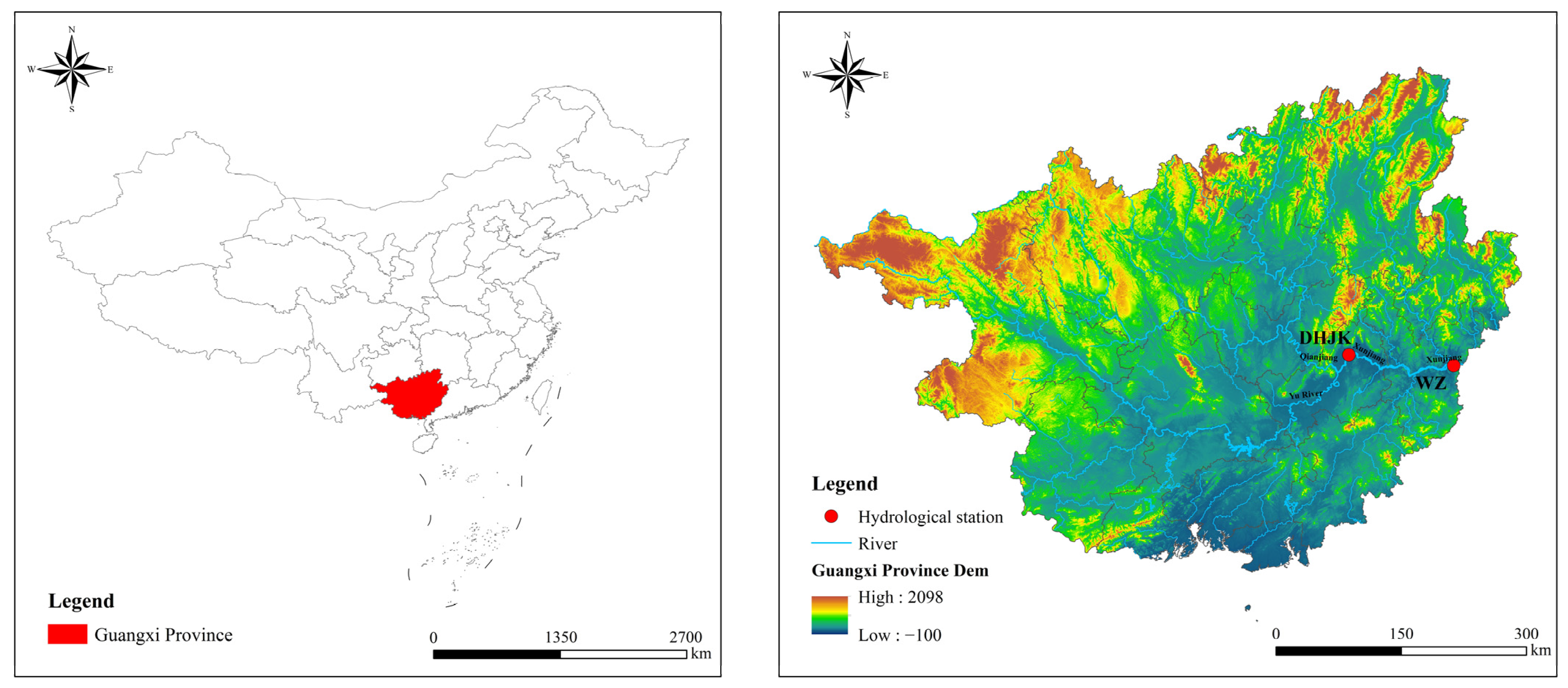
2.1. Overview of the Study Area

The Xijiang River, historically known as Yu Shui, Langshui, and Pangjiang, stands as the largest river system within the Pearl River Basin and the third longest river in China, spanning a total length of 2214 km, trailing only the Yangtze River and the Yellow River. The drainage area reaches 353,100 km², as the river traverses five provinces and autonomous regions. Renowned for its abundant water conservancy and hydraulic resources, the Xijiang River has significantly contributed to agricultural irrigation, river transportation, and power generation in coastal regions. The main streams from upstream to downstream are the Nanpan River, Hongshui River, Qian River, Xun River, and Xijiang River. Situated within the typical subtropical monsoon climate zone, the region experiences substantial annual runoff fluctuations, particularly during the flood season spanning April to September, which accounts for 72–88% of the yearly runoff. The terrain predominantly slopes from northwest to southeast.

The Wuzhou Station, a pivotal control station located in Guangxi, was established in 1900, with flow measurements commencing in 1915. Wuzhou Station records an annual average runoff of approximately 219.9 billion cubic meters, representing 95.6% of the total annual runoff of Xijiang Sixian Jiao. Monthly runoff distribution mirrors that of the Dahuangjiangkou Station, yet the period from May to October contributes 81.2% of the annual runoff, influenced by the Guijiang River.

2.2. Data Sources

This paper utilizes the recorded series of daily runoff data from the Dahuangjiangkou and Wuzhou stations spanning the period from 2003 to 2007 for runoff prediction. The daily runoff data for both stations are sourced from the Zhujiang Water Conservancy Commission, adhering to national standards for measurement and testing, ensuring high reliability and authenticity. The spatial distribution of the two sites is illustrated in Figure 1, with pertinent statistical characteristics detailed in

Table 1. Statistical characteristics of daily runoff series of selected hydrological stations.

Station	Sequence Length/d	Daily Runoff Series Statistics (m3/s)
		Maximum Value	Minimum Value	Mean Value	Standard Deviation
DHJK	1826	42,400	576	4552	4943
WZ	1826	53,300	964	5463	5786

. To uphold the model’s training and testing reliability, 70% of the data preceding each hydrological station is allocated as the training set, while the remaining 30% is designated as the test set for predictive analysis. Effective interpolation processing is carried out for some missing data.

3. Research Methods

This section mainly introduces the structure of RNN, LSTM, GRU, SVM, RF, FA, and FA-LSTM models. By explaining these models, readers can gain a more comprehensive understanding of the analytical tools and techniques used in this article.

3.1. RNN Model Introduction

Recurrent neural networks (RNNs) [46] are neural networks designed for processing sequential data. A key feature of RNNs is the incorporation of cyclic connections between hidden layers, enabling each hidden layer unit to consider the output from the previous time step when processing input at each time step, thereby capturing temporal dependencies in sequential data. In RNNs, the hidden layer neurons are interconnected by new weights, linking the neurons across hidden layers to the neurons from the previous time step in the sequence. The structure of the RNN model is depicted in Figure 2.

The mathematical expression for the hidden layer neuron is represented by Formula (1):

$$h_t=f\left(W_x{x}_t+W_s{h}_{t-1}+b_h\right)$$

(1)

For the output layer, the mathematical expression is given by Equation (2):

$$y_t=W_y{h}_t+b_y$$

(2)

where f represents the activation function; w denotes the weight matrix; x_t signifies the time series value at time t at the input end; b_h stands for the bias vector of the hidden state; and b_y represents the bias vector of the output.

3.2. LSTM Model Introduction

Long short-term memory (LSTM) [47] is a modified RNN structure tailored to addressing vanishing and exploding gradient issues, enhancing the capture of long-term dependencies. By integrating sophisticated gating mechanisms, LSTM effectively manages information retention, forgetting, and gradient flow over extended sequences. The typical structure of the LSTM model memory unit is illustrated in Figure 3.

The specific calculation process is expressed as:

$$f_t=\sigma (W_f[h_{t-1},x_t]+b_f)$$

(3)

$$i_t=\sigma (W_i[h_{t-1},x_t]+b_i)$$

(4)

$$C_t^{\prime }=tanh(W_c[h_{t-1},x_t]+b_c)$$

(5)

$$C_t=f_t\otimes C_{t-1}+i_t\otimes C_{t-1}^{\prime }$$

(6)

$$O_t=\sigma (W_o[h_{t-1},x_t]+b_o)$$

(7)

$$h_t=o_{t}tanh\otimes C_{t}t$$

(8)

where x_t represents the input vector; h_t−1 denotes the output information from the previous unit state; $\sigma$ signifies the sigmoid activation function; $\otimes$ denotes vector multiplication; W_f, W_i, W_c, and W_o are the weight matrices of the neural network; b_f, b_i, b_c, and b_o represent the bias vectors.

3.3. GRU Model Introduction

Gated Recurrent Units (GRUs) [48], a variant of RNNs, are designed to address gradient challenges. Compared to LSTM, GRUs streamline gating mechanisms from three to two, enhancing operational efficiency while preserving model accuracy. The internal structure of GRUs is depicted in Figure 4. Update gates regulate the transfer of information from memory cells of the previous moment to the current moment, determining the retention of past memory. Reset gates control the integration of information from memory cells of the previous moment into the current moment’s input, facilitating selective memory updates.

The specific calculation process is expressed as:

$$r_t=\sigma \left(W_{rh}{h}_{t-1}+W_{zx}{x}_t\right)$$

(9)

$$z_t=\sigma \left(W_{zh}{h}_{t-1}+W_{zx}{x}_t\right)$$

(10)

$$\overline{h_t}=\tanh \left(W_{hh}\left(r_t\odot h_{t-1}\right)+W_{hx}{x}_t\right)$$

(11)

$$h_t=h_{t-1}\odot z_t+\overline{h_t}\odot \left(1-z_t\right)$$

(12)

$$t=\sigma \left(W_{qh}{h}_t\right)$$

(13)

where tanh and $\sigma$ denote the tangent and sigmoid activation functions, respectively; W signifies the weight of the variable; $\odot$ represents the element-wise product; t signifies the output variable value of the output layer; W_qh denotes the weight coefficient of the output layer; W_rh represents the weight coefficient of the reset gate; W_zh signifies the weight coefficient of the update gate; W_hh denotes the weight coefficient of the hidden state in the previous moment; and W_hx represents the weight coefficient that conceals the candidate state at the current moment.

3.4. SVM Model Introduction

Support vector machines (SVMs) [49] are classical machine learning models utilized for classification and regression tasks. SVMs aim to identify an optimal hyperplane that separates data points of different categories, minimizing classification errors while maximizing margins. The principle of SVMs is illustrated in Figure 5. For nonlinear problems, SVMs employ kernel techniques to map data to a high-dimensional space, rendering data linearly separable. In regression tasks, SVMs can model nonlinear relationships effectively.

In this study, SVMs are applied to the nonlinear regression problem of runoff prediction, and its regression function is expressed as follows:

$$f(x)={\displaystyle \sum _{i=1}^n{\alpha }_{i}K\left(x,x_i\right)+b}$$

(14)

where $\alpha$ represent Lagrange multipliers; x_i denotes the support vector; $K$ signifies the kernel function, which must satisfy Mercer’s condition; b represents the offset term. Common kernel functions include the linear kernel, radial basis kernel, and others.

3.5. RF Model Introduction

Random forest (RF) [50] is an ensemble learning method comprising multiple decision trees. During training, samples and features are randomly selected from raw data to train multiple decision trees. Each decision tree in the random forest makes predictions for new input data in classification or regression tasks, with the final result being determined by voting or averaging these predictions. The basic structure of a simple RF model is depicted in Figure 6.

3.6. Firefly Algorithm

The firefly algorithm (FA) [51] is a heuristic optimization algorithm inspired by the behavior of fireflies in nature. Mimicking firefly behavior in search and reproduction, FA utilizes mutual attraction and light to seek optimal solutions. The algorithm iteratively updates firefly positions and brightness, enabling brighter fireflies to attract darker ones, facilitating global optimal solution search. The FA process involves elements of brightness and attraction, with brightness reflecting firefly position and attraction determining movement distance.

The brightness of fireflies is defined as:

$$I_{ij}(r_{ij})=I_i{e}^{-\gamma r_{ij}^2}$$

(15)

where I_i denotes the maximum fluorescence brightness of firefly i, correlated with the objective function value. Higher objective function values correspond to increased brightness of the firefly; $\gamma$ represents the light absorption coefficient, with fluorescence diminishing gradually with distance and media absorption, typically set as a constant; r_ij signifies the distance between firefly i and firefly j, which is defined as:

$$r_{ij}=\overrightarrow{x_i}-\overrightarrow{x_j}=\sqrt{{\displaystyle \sum _{k=1}^d{(x_{i,k}-x_{j,k})}^2}}$$

(16)

According to the relative brightness formula, the attraction degree of firefly i to firefly j is:

$${\beta }_{ij}(r_{ij})={\beta }_0{e}^{-\gamma r_{ij}^2}$$

(17)

where ${\beta }_0$ is the attraction of fireflies at r_ij = 0.

Firefly j is attracted by firefly i and moves towards it. The position update formula is as follows:

$$\overrightarrow{x_j}(t+1)=\overrightarrow{x_j}(t)+{\beta }_{ij}(r_{ij})(\overrightarrow{x_i}(t)-\overrightarrow{x_j}(t))+\alpha \overrightarrow{{\epsilon }_j}$$

(18)

where t represents the number of algorithm iterations; $\overrightarrow{x_i}$ and $\overrightarrow{x_j}$ denote the position coordinates of fireflies; ${\beta }_{ij}(r_{ij})$ signifies the attraction between fireflies; $\alpha$ is a constant and generally acceptable [0, 1]; $\overrightarrow{{\epsilon }_j}$ denotes a random number vector.

The FA algorithm is detailed in Figure 7, where fireflies are initially distributed uniformly and randomly in the search space, attracted by brighter fireflies to optimize the solution iteratively.

3.7. Model Construction and Parameter Setting

3.7.1. Model Construction

The constructed dataset is divided into a training set and a test set. The training set comprises data from 1 January 2003 to 2 July 2006, for model training purposes. The test set consists of data from 3 July 2006 to 31 December 2007, and is utilized to evaluate the predictive performance of the model. In the forecasting process, the historical runoff is used as input, and the predicted runoff is used as output. The model employs the rolling window method to predict the runoff on day t. This method uses the runoff data from the previous t − 1 day as input to predict the runoff on day t. The window is then shifted to predict the runoff on day t + 1 by utilizing the data from day t − 3 to day t as the new input feature. This process is repeated until all the data is covered.

Runoff forecasting is subject to various influencing factors and inherent instability. This study selects the LSTM model, known for its exceptional performance in runoff prediction, as the foundational model. To enhance the LSTM model’s predictive efficacy, the FA is employed to optimize key parameters such as learning rate, training batch size, number of hidden layer elements, and iteration times. This optimization process yields the optimal combination of model parameters. The flowchart of the FA-LSTM hybrid model is illustrated in Figure 8.

3.7.2. Model Parameter Setting

We adopted a unified parameter adjustment method; that is, we calculated the best parameters for the data set in this paper through cross-validation and multiple trials. The main settings of each model are as follows:

The key hyperparameters of the LSTM model include the learning rate, training batch size, number of hidden layer units, and iteration count. The learning rate governs the model’s complexity and generalization ability, the training batch size influences training speed and effectiveness, the number of hidden layer units impacts model representation capacity, and the iteration count affects model fitting. Figure 9 illustrates that when the learning rate is 0.1 or less, the R² indicators of both the model training set and test set remain stable, resulting in better model fit. Conversely, if the learning rate exceeds 0.1, the indicators decrease significantly, indicating that the value should not be excessively high. Model performance varies with changes in batch size. A batch size within the range of 24 to 64 (inclusive) yields relatively good model performance, while increasing the batch size to 80 to 120 (inclusive) leads to a decline in performance. When the number of hidden layer units surpasses 105, the R² indices for both training and test sets are consistently high and exhibit minimal fluctuation. With the increase of the number of iterations, the R² index of the model was observed to be gradually stable between 110 and 200 iterations, indicating that the model had learned the data features well, and further increasing the number of iterations had little impact on the improvement of the model accuracy. Consequently, to ensure optimal model fitting and enhance predictive performance, the LSTM model’s hyperparameters are set as follows: learning rate of 0.01, training batch size of 64, number of hidden layer units at 105, and iteration count of 110.

In constructing the FA-LSTM hybrid model, FA is utilized to optimize the aforementioned hyperparameters within specified ranges. The FA parameters are configured with a firefly population of 10, light absorption coefficient of 0.005, 200 iterations, and default values for other parameters. RNN, GRU and LSTM models have the same activation function and optimizer settings, which are RELU and Adam. The RNN model is a single-layer model with 48 neuron nodes and 150 iteration times. The GRU model is a single-layer model with 32 neuron nodes, 0.01 learning rate, and 200 iteration times. In the SVM model, the radial basis function (RBF) serves as the kernel function, with the penalty parameter c set to 600 and the ε parameter set to 2. For the RF model, each forest comprises 6 decision trees, with a maximum tree depth of 5 and a minimum branching sample node of 3.

4. Case Analysis

4.1. Model Evaluation Index

To assess prediction accuracy and effectiveness, the study employs average absolute error (MAE), root mean square error (RMSE), determination coefficient (R²), and Kling–Gupta efficiency coefficient (KGE) as evaluation metrics. The specific calculation formula is as follows:

$$MAE={\displaystyle \frac{1}{n}}{\displaystyle \sum _{i=1}^n\left|y_i-\overline{\overline{y_i}}\right|}$$

(19)

$$RMSE=\sqrt{{\displaystyle \frac{1}{n}}{\displaystyle \sum _{i=1}^n(y_i-\overline{\overline{y_i}}{)}^2}}$$

(20)

$$R^2=1-{\displaystyle \frac{{\displaystyle \sum _{i=1}^n{\left(y_i-\overline{\overline{y_i}}\right)}^2}}{{\displaystyle \sum _{i=1}^n{\left(y_i-\overline{y}\right)}^2}}}$$

(21)

$$KGE=1-\sqrt{(r-1{)}^2+({\displaystyle \frac{s}{s_0}}-1{)}^2+({\displaystyle \frac{e}{\overline{y}}}-1{)}^2}$$

(22)

where $y_i$ is the measured value of the i-day runoff, $\overline{\overline{y_i}}$ is the predicted value of the i-day runoff, $\overline{y}$ is the average value of the observed daily runoff, n is the length of the runoff time series, r is the correlation coefficient, s₀ is the standard deviation of the observed daily runoff, and e is the average value of the predicted daily runoff.

Mean absolute error (MAE) represents the average value of absolute errors, effectively reflecting the actual error in predictions. Its range is from 0 to positive infinity, with smaller values indicating lower model errors. Root mean square error (RMSE) is the square root of the mean squared error, with smaller values indicating better model fitting and higher accuracy. The determination coefficient R² ranges from 0 to 1, with values closer to 1 indicating higher predictive accuracy. KGE comprehensively considers the correlation between the model prediction results and the measured data, and the difference between the mean and standard deviation. The closer the value is to 1, the better the model performance is.

4.2. Comparison and Analysis of Model Results

To showcase the accuracy of the hybrid model proposed in this study for daily runoff prediction, we compared the performance of various technical models in the Dahuangjiangkou river estuary station and Wuzhou Hydrological Station in the Xijiang River Basin, including RNNs, LSTM, GRUs, SVMs, RF, and the FA-LSTM model proposed in this paper. The FA-LSTM model was used to carry out the generalization experiment in Qianjiang, Wuxuan, and Guigang hydrology stations, along with an analysis of the FA-LSTM model’s performance over a prediction period of 1–5 days.

4.2.1. Runoff Prediction Results of the Model

The evaluation metrics for the six models are summarized in

Table 2. Evaluation results of each model during training and testing.

Station	Model	Training Set				Test Set
		MAE (103 m3/s)	RMSE (103 m3/s)	R2	KGE	MAE (103 m3/s)	RMSE (103 m3/s)	R2	KGE
DHJK	FA-LSTM	0.426	0.850	0.972	0.965	0.455	0.871	0.966	0.965
	RNN	0.564	1.214	0.935	0.917	0.596	1.283	0.933	0.917
	LSTM	0.490	1.046	0.952	0.952	0.495	1.101	0.950	0.953
	GRU	0.560	1.130	0.949	0.943	0.574	1.141	0.942	0.942
	SVM	0.651	1.248	0.932	0.908	0.663	1.319	0.929	0.891
	RF	0.562	1.164	0.943	0.940	0.575	1.208	0.939	0.938
WZ	FA-LSTM	0.445	1.117	0.968	0.956	0.330	0.748	0.971	0.960
	RNN	0.704	1.581	0.936	0.933	0.465	1.027	0.946	0.935
	LSTM	0.615	1.454	0.946	0.945	0.427	0.949	0.954	0.947
	GRU	0.638	1.507	0.942	0.938	0.454	0.988	0.950	0.940
	SVM	0.766	1.665	0.929	0.916	0.541	1.090	0.939	0.908
	RF	0.733	1.614	0.934	0.929	0.516	1.053	0.943	0.929

. The FA-LSTM model demonstrates superior prediction performance compared to RNN, LSTM, GRU, SVM, and RF models overall. In both the training and verification periods, the fitting accuracy at Dahuangjiangkou Station ranks as follows: FA-LSTM, LSTM, GRUs, RF, RNNs, SVMs. At Wuzhou Station, the order is FA-LSTM, LSTM, GRUs, RNNs, RF, and SVMs. Notably, the FA-LSTM model exhibits the best fitting performance across all stations, with R² and KGE values approaching 1 and minimized MAE and RMSE values. Comparing the single models, LSTM performs best for both stations, followed by GRUs, while SVMs show the least favorable fitting effect, and RNN and RF models exhibit varying performances in different scenarios.

For Dahuangjiangkou Station, compared with RNN, LSTM, GRU, SVM, and RF models, the R² values of the FA-LSTM model during the test period increased by 3.54%, 1.68%, 2.54%, 3.98%, and 2.87%, respectively. The KGE value increased by 5.23%, 1.26%, 2.44%, 8.31%, and 2.88% respectively. RMSE value decreased by 32.11%, 20.89%, 23.66%, 33.97%, and 27.90%, and MAE value decreased by 23.66%, 8.08%, 20.73%, 31.37%, and 20.87%, respectively. For Wuzhou Station, compared with RNN, LSTM, GRU, SVM, and RF models, the R² values of FA-LSTM model during the test period increased by 2.64%, 1.78%, 2.21%, 3.41%, and 2.97%, respectively. KGE value increased by 2.67%, 1.37%, 2.13%, 5.73%, and 3.34% respectively. RMSE value decreased by 27.17%, 21.18%, 24.29%, 31.38%, and 28.96%, while MAE value decreased by 29.03%, 22.72%, 27.31%, 39.00%, and 36.05%, respectively. This indicates that FA has a positive effect on parameter tuning.

Figure 10 illustrates the runoff forecast results of six models at two stations. The consistency in the general trend of predicted and observed values across different models indicates the reliability and effectiveness of the adopted model in runoff prediction.

For a more in-depth analysis of each model’s prediction performance during the verification period, Figure 11 presents scatter plots of predicted and observed values for Dahuangjiangkou and Wuzhou stations, with red lines representing linear fitting lines. Observing Figure 11 reveals noticeable deviations between the fitting lines of the five single models and the data points, with a relatively scattered scatter distribution. This suggests that the overall prediction ability of these models is limited, particularly when predicting extreme values. In contrast, the FA-LSTM model exhibits a concentrated scatter distribution, showcasing improved overall prediction and extreme value prediction performance, indicating enhanced prediction accuracy.

4.2.2. Model Generalization Experiment

To further validate the generalization of the proposed FA-LSTM model, we applied the trained model to the daily runoff data of Qianjiang, Guigang, and Wuxuan hydrographic stations in the Xijiang River Basin from 1961 to 1970. The dataset is complete without missing values, with the first 70% of data from each hydrologic station used as the training set and the remaining 30% as the test set. Maintaining consistent parameter settings ensures the experiment’s repeatability, facilitating an objective comparison of predicted performance across different hydrology stations. The prediction results of the FA-LSTM model on the training and test sets of each hydrographic station are detailed in

Table 3. Prediction results of FA-LSTM model for each hydrographic station.

Station	Model	Training Set				Test Set
		MAE (103 m3/s)	RMSE (103 m3/s)	R2	KGE	MAE (103 m3/s)	RMSE (103 m3/s)	R2	KGE
QJ	FA-LSTM	0.198	0.484	0.970	0.984	0.157	0.411	0.973	0.985
WX	FA-LSTM	0.309	0.850	0.963	0.980	0.426	1.105	0.960	0.978
GG	FA-LSTM	0.099	0.224	0.977	0.962	0.183	0.345	0.975	0.961

and Figure 12a–c. It can be seen from the prediction results that the prediction accuracy of FA-LSTM model for daily runoff series is basically stable. The model consistently achieves a prediction accuracy of 0.96 or higher, underscoring its adaptability across diverse hydrological stations and its robust predictive capabilities.

4.2.3. The Prediction Performance of the Optimal Model under Different Prediction Periods

Based on the preceding analysis, it is evident that the FA-LSTM model exhibits superior predictive performance. To delve deeper into the model’s accuracy across varying prediction periods, forecasts ranging from 1 to 5 days were scrutinized at Dahuangjiangkou Station and Wuzhou Station. The prediction results for these hydrographic stations at different forecast periods are detailed in

Table 4. The prediction effect of FA-LSTM model under different prediction periods.

Station	Model	Error Indicator	Forecast Period
			1 Day	2 Days	3 Days	4 Days	5 Days
DHJK	FA-LSTM	MAE (103 m3/s)	0.455	0.699	0.803	0.980	1.072
		RMSE (103 m3/s)	0.871	1.360	1.747	2.042	2.304
		R2	0.966	0.916	0.862	0.811	0.760
		KGE	0.965	0.930	0.915	0.837	0.811
WZ	FA-LSTM	MAE (103 m3/s)	0.330	0.520	0.650	0.769	0.843
		RMSE (103 m3/s)	0.748	1.128	1.475	1.751	1.995
		R2	0.971	0.935	0.888	0.843	0.796
		KGE	0.960	0.939	0.885	0.861	0.821

and Figure 13. Notably, at Dahuangjiangkou Station, the R² values for 1 to 5 days decrease by 5.18%, 5.90%, 5.92%, and 6.29% respectively, while the KGE values decrease by 3.63%, 1.61%, 8.52%, and 3.11% respectively. Similarly, at Wuzhou Station, the R² values for 1 to 5 days decrease by 3.71%, 5.03%, 5.07%, and 5.58% respectively, with the KGE values decreasing by 2.19%, 5.75%, 2.71%, and 4.65% respectively.

5. Discussion

Runoff prediction is pivotal for natural resource management and environmental conservation. This study compares the performance of various models, including RNN, LSTM, GRU, SVM, RF, and FA-LSTM. The evaluation outcomes of the identical prediction cycle test set are delineated in the Taylor diagram (Figure 14) and the Violin diagram (Figure 15), accentuating the exceptional predictive prowess of the FA-LSTM model across diverse hydrographic stations. Subsequently, the FA-LSTM model’s accuracy and stability are assessed over different forecasting periods, demonstrating its sustained predictive efficacy despite a slight performance decline. FA is an efficient optimization technique. Optimization of LSTM model parameters (learning rate, number of hidden layer elements, etc.) by FA can improve the integrity of the model and reduce the risk of overfitting and underfitting. Unlike process-based hydrological models reliant on intricate hydrological mechanisms, FA-LSTM models operate independently of such physical constraints. Moreover, while traditional hydrological models demand extensive hydrological data, FA-LSTM models exhibit versatility by training on limited time series data, such as historical runoff and precipitation, to construct intricate models efficiently. However, this paper also has some limitations. The escalating unpredictability of weather patterns due to global climate change has intensified extreme flood and drought occurrences, amplifying uncertainty in river runoff forecasts. Acknowledging the complexity of flood and drought genesis involving multifaceted interactions, the reliance solely on historical runoff data in the model may not encapsulate these intricate hydrometeorological processes comprehensively. Future research avenues could entail incorporating additional input variables to enhance the model’s predictive capacity for extreme weather events. Furthermore, this study is based on the data from 2003 to 2007, and previous studies have shown that flow rate is affected by multiple factors such as precipitation, temperature and potential evaporation [52,53]. Because the data used predates many observed climate changes, the results may not accurately reflect current runoff, and future studies may need to collect updated data for further research.

In this study, FA-LSTM model has made some progress in the prediction effect, and it can become a framework for machine learning applications, which can be further optimized or integrated with new technologies in the future to promote the research of more efficient hydrological prediction methods.

6. Conclusions

To enhance the precision of runoff prediction, this paper introduces a FA-LSTM hybrid model. The model’s performance is evaluated using daily runoff data from Dahuangjiangkou Station and Wuzhou Station in the Xijiang River Basin. Additionally, a generalization experiment is conducted by applying the model to Qianjiang Station, Wuxuan Station, and Guigang Station in the same basin:

(1) Model Performance Comparison: A comparative analysis of the FA-LSTM mixed model with RNN, LSTM, GRU, SVM, and RF models demonstrates superior R² values of 0.966 and 0.971, and KGE values of 0.965 and 0.960, for Dahuangjiangkou Station and Wuzhou Station, respectively. These values outperform other single models, yielding more accurate predictions. Further examination of the single models indicates that the LSTM model performs best, followed by GRUs, while SVMs exhibit the least favorable performance. RNNs and RF models demonstrate varying performances across different scenarios.

(2) Generalization Experiment Results: The FA-LSTM model is applied to Qianjiang, Wuxuan, and Guigang hydrological stations, achieving prediction accuracies of 0.96 or higher. This outcome underscores the model’s adaptability across diverse hydrological stations and its robustness.

(3) Forecast Period Analysis: A detailed comparison of runoff prediction over forecast periods of 1–5 days is conducted to explore the variation in prediction accuracy of the FA-LSTM model at the two hydrological stations. The findings reveal a trend of decreasing R² and KGE values as the prediction period extends. Specifically, at Dahuangjiangkou Station, the R² value decreased from 0.966 to 0.760, the KGE value decreased from 0.965 to 0.811, the MAE increased from 0.455 to 1.072, and the RMSE increased from 0.871 to 2.304 over the 1st to 5th day. Similarly, at Wuzhou Station, the R² decreased from 0.971 to 0.796, KGE decreased from 0.960 to 0.821, MAE increased from 0.330 to 0.843, and RMSE increased from 0.748 to 1.995. Despite the gradual decline in model accuracy, it continues to exhibit a viable predictive capability.

Based on the above results, the FA-LSTM model can be regarded as an effective runoff prediction tool, which provides a new method to improve the accuracy of daily runoff forecast.

References

1. Solaimani, K. Rainfall-runoff prediction based on artificial neural network (a case study: Jarahi watershed). Am.-Eurasian J. Agric. Environ. Sci. 2009, 5, 856–865. [Google Scholar]
2. Li, F.F.; Cao, H.; Hao, C.F.; Qiu, J. Daily streamflow forecasting based on flow pattern recognition. Water Resour. Manag. 2021, 35, 4601–4620. [Google Scholar] [CrossRef]
3. Wu, J.H.; Wang, Z.C.; Dong, J.H.; Cui, X.F.; Tao, S.; Chen, X. Robust runoff prediction with explainable artificial intelligence and meteorological variables from deep learning ensemble model. Water Resour. Res. 2023, 59, e2023WR035676. [Google Scholar] [CrossRef]
4. Mao, G.Q.; Wang, M.; Liu, J.G.; Wang, Z.F.; Wang, K.; Meng, Y.; Zhong, R.; Li, Y. Comprehensive comparison of artificial neural networks and long short-term memory networks for rainfall-runoff simulation. Phys. Chem. Earth Parts A/B/C 2021, 123, 103026. [Google Scholar] [CrossRef]
5. Han, H.; Morrison, R.R. Improved runoff forecasting performance through error predictions using a deep-learning approach. J. Hydrol. 2022, 608, 127653. [Google Scholar] [CrossRef]
6. Lei, X.H.; Wang, H.; Yang, M.X.; Gui, Z.L. Research Progress on Meteorological Hydrological Forecasting under Changing Environments. J. Hydraul. Eng. 2018, 49, 9–18. (In Chinese) [Google Scholar]
7. Zhu, S.; Zhou, J.Z.; Ye, L.; Meng, C.Q. Streamflow estimation by support vector machine coupled with different methods of time series decomposition in the upper reaches of Yangtze River, China. Environ. Earth Sci. 2016, 75, 531. [Google Scholar] [CrossRef]
8. Wu, J.H.; Wang, Z.C.; Hu, Y.; Tao, S.; Dong, J.H. Runoff forecasting using convolutional neural networks and optimized bi-directional long short-term memory. Water Resour. Manag. 2023, 37, 937–953. [Google Scholar] [CrossRef]
9. Kalra, A.; Miller, W.P.; Lamb, K.W.; Ahmad, S.; Piechota, T. Using large-scale climatic patterns for improving long lead time streamflow forecasts for Gunnison and San Juan River Basins. Hydrol. Process. 2013, 27, 1543–1559. [Google Scholar] [CrossRef]
10. Lin, G.F.; Chou, Y.C.; Wu, M.C. Typhoon flood forecasting using integrated two-stage support vector machine approach. J. Hydrol. 2013, 486, 334–342. [Google Scholar] [CrossRef]
11. Xu, X.Y.; Yang, D.; Yang, H.; Lei, H. Attribution analysis based on the Budyko hypothesis for detecting the dominant cause of runoff decline in Haihe basin. J. Hydrol. 2014, 510, 530–540. [Google Scholar] [CrossRef]
12. Van, S.P.; Le, H.M.; Thanh, D.V.; Dang, T.D.; Loc, H.H.; Anh, D.T. Deep learning convolutional neural network in rainfall–runoff modelling. J. Hydroinform. 2020, 22, 541–561. [Google Scholar] [CrossRef]
13. Liu, Y.; Zhang, T.; Kang, A.Q.; Li, J.Z.; Lei, X.H. Research on runoff simulations using deep-learning methods. Sustainability 2021, 13, 1336. [Google Scholar] [CrossRef]
14. Osman, A.; Afan, H.A.; Allawi, M.F.; Jaafar, O.; Noureldin, A.; Hamzah, F.M.; Ahmed, A.N.; El-Shafie, A. Adaptive Fast Orthogonal Search (FOS) algorithm for forecasting streamflow. J. Hydrol. 2020, 586, 124896. [Google Scholar] [CrossRef]
15. Wu, Y.Q.; Wang, Q.H.; Li, G.; Li, J.D. Data-driven runoff forecasting for Minjiang River: A case study. Water Supply 2020, 20, 2284–2295. [Google Scholar] [CrossRef]
16. Moosavi, V.; Fard, Z.G.; Vafakhah, M. Which one is more important in daily runoff forecasting using data driven models: Input data, model type, preprocessing or data length? J. Hydrol. 2022, 606, 127429. [Google Scholar] [CrossRef]
17. Wang, J.J.; Shi, P.; Jiang, P.; Hu, J.W.; Qu, S.; Chen, X.Y.; Chen, Y.B.; Dai, Y.Q.; Xiao, Z.W. Application of BP neural network algorithm in traditional hydrological model for flood forecasting. Water 2017, 9, 48. [Google Scholar] [CrossRef]
18. Sivapragasam, C.; Liong, S.Y.; Pasha, M.F.K. Rainfall and runoff forecasting with SSA–SVM approach. J. Hydroinform. 2001, 3, 141–152. [Google Scholar] [CrossRef]
19. Li, M.; Zhang, Y.Q.; Wallace, J.; Campbell, E. Estimating annual runoff in response to forest change: A statistical method based on random forest. J. Hydrol. 2020, 589, 125168. [Google Scholar] [CrossRef]
20. Zhang, J.; Chen, X.; Khan, A.; Zhang, Y.K.; Kuang, X.; Liang, X.; Taccari, M.; Nuttall, J. Daily runoff forecasting by deep recursive neural network. J. Hydrol. 2021, 596, 126067. [Google Scholar] [CrossRef]
21. He, F.F.; Wan, Q.J.; Wang, Y.Q.; Wu, J.; Zhang, X.Q.; Feng, Y. Daily Runoff Prediction with a Seasonal Decomposition-Based Deep GRU Method. Water 2024, 16, 618. [Google Scholar] [CrossRef]
22. Tabas, S.S.; Samadi, S. Variational Bayesian dropout with a Gaussian prior for recurrent neural networks application in rainfall–runoff modeling. Environ. Res. Lett. 2022, 17, 065012. [Google Scholar] [CrossRef]
23. Gao, S.; Huang, Y.F.; Zhang, S.; Han, J.C.; Wang, G.Q.; Zhang, M.X.; Lin, Q.S. Short-term runoff prediction with GRU and LSTM networks without requiring time step optimization during sample generation. J. Hydrol. 2020, 589, 125188. [Google Scholar] [CrossRef]
24. Sheng, Z.Y.; Wen, S.P.; Feng, Z.K.; Shi, K.B.; Huang, T.W. A Novel Residual Gated Recurrent Unit Framework for Runoff Forecasting. IEEE Internet Things J. 2023, 10, 12736–12748. [Google Scholar] [CrossRef]
25. Ayzel, G.; Heistermann, M. The effect of calibration data length on the performance of a conceptual hydrological model versus LSTM and GRU: A case study for six basins from the CAMELS dataset. Comput. Geosci. 2021, 149, 104708. [Google Scholar] [CrossRef]
26. Kratzert, F.; Klotz, D.; Brenner, C.; Schulz, K.; Herrnegger, M. Rainfall–runoff modelling using long short-term memory (LSTM) networks. Hydrol. Earth Syst. Sci. 2018, 22, 6005–6022. [Google Scholar] [CrossRef]
27. Li, W.; Kiaghadi, A.; Dawson, C. High temporal resolution rainfall–runoff modeling using long-short-term-memory (LSTM) networks. Neural Comput. Appl. 2021, 33, 1261–1278. [Google Scholar] [CrossRef]
28. Sabzipour, B.; Arsenault, R.; Troin, M.; Martel, J.L.; Brissette, F.; Brunet, F.; Mai, J. Comparing a long short-term memory (LSTM) neural network with a physically-based hydrological model for streamflow forecasting over a Canadian catchment. J. Hydrol. 2023, 627, 130380. [Google Scholar] [CrossRef]
29. Yin, Z.K.; Liao, W.H.; Wang, R.J.; Lei, X.H. Rainfall-Runoff Simulation and Forecasting Based on Long Short-Term Memory Neural Network (LSTM). South—North Water Divers. Water Sci. Technol. 2019, 17, 1–9. (In Chinese) [Google Scholar]
30. Li, J.X.; Qian, K.X.; Liu, Y.; Yan, W.; Yang, X.Y.; Luo, G.P.; Ma, X.F. LSTM-based model for predicting inland river runoff in arid region: A case study on Yarkant River, Northwest China. Water 2022, 14, 1745. [Google Scholar] [CrossRef]
31. Yang, L.; Shami, A. On hyperparameter optimization of machine learning algorithms: Theory and practice. Neurocomputing 2020, 415, 295–316. [Google Scholar] [CrossRef]
32. Luo, G. A review of automatic selection methods for machine learning algorithms and hyper-parameter values. Netw. Model. Anal. Health Inform. Bioinform. 2016, 5, 1–16. [Google Scholar] [CrossRef]
33. Wu, J.W.; Chen, X.Y.; Zhang, H.; Xiong, L.D.; Lei, H.; Deng, S.H. Hyperparameter optimization for machine learning models based on Bayesian optimization. J. Electron. Sci. Technol. 2019, 17, 26–40. [Google Scholar]
34. Chu, H.B.; Wang, Z.Q.; Nie, C. Monthly Streamflow Prediction of the Source Region of the Yellow River Based on Long Short-Term Memory Considering Different Lagged Months. Water 2021, 16, 593. [Google Scholar] [CrossRef]
35. Alqahtani, F. AI-driven improvement of monthly average rainfall forecasting in Mecca using grid search optimization for LSTM networks. J. Water Clim. Chang. 2024, 15, 1439–1458. [Google Scholar] [CrossRef]
36. Yang, X.Z.; Maihemuti, B.; Simayi, Z.; Saydi, M.; Na, L. Prediction of glacially derived runoff in the muzati river watershed based on the PSO-LSTM model. Water 2022, 14, 2018. [Google Scholar] [CrossRef]
37. Xu, Y.H.; Hu, C.H.; Wu, Q.; Jian, S.Q.; Li, Z.H.; Chen, Y.Q.; Zhang, G.D.; Zhang, Z.X.; Wang, S. Research on particle swarm optimization in LSTM neural networks for rainfall-runoff simulation. J. Hydrol. 2022, 608, 127553. [Google Scholar] [CrossRef]
38. Aderyani, F.R.; Mousavi, S.J.; Jafari, F. Short-term rainfall forecasting using machine learning-based approaches of PSO-SVR, LSTM and CNN. J. Hydrol. 2022, 614, 128463. [Google Scholar] [CrossRef]
39. Wang, X.J.; Wang, Y.P.; Yuan, P.X.; Wang, L.; Cheng, D.L. An adaptive daily runoff forecast model using VMD-LSTM-PSO hybrid approach. Hydrol. Sci. J. 2021, 66, 1488–1502. [Google Scholar] [CrossRef]
40. Li, W.Z.; Liu, C.S.; Hu, C.H.; Niu, C.J.; Li, R.X.; Li, M.; Xu, Y.Y.; Tian, L. Application of a hybrid algorithm of LSTM and Transformer based on random search optimization for improving rainfall-runoff simulation. Sci. Rep. 2021, 14, 11184. [Google Scholar] [CrossRef]
41. Naganna, S.R.; Marulasiddappa, S.B.; Balreddy, M.S.; Yaseen, Z.M. Daily scale streamflow forecasting in multiple stream orders of Cauvery River, India: Application of advanced ensemble and deep learning models. J. Hydrol. 2023, 626, 130320. [Google Scholar] [CrossRef]
42. Cong, Y.; Zhao, X.M.; Tang, K.; Wang, G.; Hu, Y.F.; Jiao, Y.K. FA-LSTM: A novel toxic gas concentration prediction model in pollutant environment. IEEE Access 2021, 10, 1591–1602. [Google Scholar] [CrossRef]
43. Luo, G.; Wang, X.Y.; Zhu, J.M.; Zhou, Y.Q. Quantitative detection of composite defects based on infrared technology and FA-LSTM. J. Phys. Conf. Ser. 2024, 2770, 012012. [Google Scholar] [CrossRef]
44. Zhu, L.Z. Short-term power load forecasting based on FA-LSTM with similar day selection. In Proceedings of the 2023 IEEE 3rd International Conference on Electronic Technology, Communication and Information, Qingdao, China, 21–24 July 2023; IEEE: Piscataway, NJ. USA, 2023; pp. 1110–1115. [Google Scholar]
45. Zhang, R.; Zheng, X. Short-term wind power prediction based on the combination of firefly optimization and LSTM. Adv. Control Appl. Eng. Ind. Syst. 2024, 6, e161. [Google Scholar] [CrossRef]
46. Elman, J.L. Finding structure in time. Cogn. Sci. 1990, 14, 179–211. [Google Scholar] [CrossRef]
47. Hochreiter, S.; Schmidhuber, J. Long short-term memory. Neural Comput. 1997, 9, 1735–1780. [Google Scholar] [CrossRef]
48. Cho, K.; Van Merriënboer, B.; Gulcehre, C.; Bahdanau, D.; Bougares, F.; Schwenk, H.; Bengio, Y. Learning phrase representations using RNN encoder-decoder for statistical machine translation. arxiv 2014, arXiv:1406.1078. [Google Scholar]
49. Gunn, S.R. Support Vector Machines for Classification and Regression. Technical Report, Image Speech and Intelligent Systems Research Group, University of Southampton. 1997. Available online: http://www.isis.ecs.soton.ac.uk/isystems/kernel/ (accessed on 28 April 2024).
50. Breiman, L. Random forests. Mach. Learn. 2001, 45, 5–32. [Google Scholar] [CrossRef]
51. Yang, X.S. Firefly algorithms for multimodal optimization. In International Symposium on Stochastic Algorithms; Springer: Berlin/Heidelberg, Germany, 2009; pp. 169–178. [Google Scholar]
52. Chen, Y.; Zhang, P.; Zhao, Y.; Qu, L.Q.; Du, P.F.; Wang, Y.G. Factors Affecting Runoff and Sediment Load Changes in the Wuding River Basin from 1960 to 2020. Hydrology 2022, 9, 198. [Google Scholar] [CrossRef]
53. Yin, L.; Wang, L.; Keim, B.D.; Konsoer, K.; Yin, Z.; Liu, M.; Zheng, W. Spatial and wavelet analysis of precipitation and river discharge during operation of the Three Gorges Dam, China. Ecol. Indic. 2023, 154, 110837. [Google Scholar] [CrossRef]
Figure 1. Location of selected hydrological control station.
Water 16 02216 g001
Figure 2. RNN model basic structure diagram.
Water 16 02216 g002
Figure 3. LSTM model basic structure diagram.
Water 16 02216 g003
Figure 4. GRU model basic structure diagram.
Water 16 02216 g004
Figure 5. SVM model basic structure diagram.
Water 16 02216 g005
Figure 6. RF model schematic.
Water 16 02216 g006
Figure 7. FA flow chart.
Water 16 02216 g007
Figure 8. FA optimizes LSTM model flow chart.
Water 16 02216 g008
Figure 9. R2 index trends of four hyperparameters of LSTM model.
Water 16 02216 g009
Figure 10. Comparison of predicted and observed runoff values.
Water 16 02216 g010
Figure 11. Scatter plots of predicted and observed values for (a) DHJK station and (b) WZ station.
Water 16 02216 g011
Figure 12. (a) Comparison of predicted and observed values at QJ station. (b) Comparison of predicted and observed values at WX station. (c) Comparison of predicted and observed values at GG station.
Water 16 02216 g012aWater 16 02216 g012bWater 16 02216 g012c
Figure 13. Prediction results of FA-LSTM model for (a) DHJK station and (b) WZ station under different forecast periods.
Water 16 02216 g013
Figure 14. Taylor diagram for (a) DHJK Station and (b) WZ station.
Water 16 02216 g014
Figure 15. Violin plots of predicted and measured values for (a) DHJK station and (b) WZ station.
Water 16 02216 g015