A Spectral Precursor Indicative of Artificial Water Reservoir-Induced Seismicity: Observations from the Xiangjiaba Reservoir, Southwestern China

Abstract

Spectral analysis is an effective tool for processing seismic signals, particularly when time-domain characteristics are challenging to capture. In this study, we developed a method using P-wave signals to calculate the power spectrum, enabling the estimation of two spectral parameters—peak frequency and shape factor—for earthquakes recorded by regional seismic networks in the Xiangjiaba (XJB) reservoir area from 2010 to 2015. The temporal evolution of the two spectral parameters was analyzed, revealing that the mean values of individual spectral parameters remain relatively stable despite variations in reservoir water levels. However, a notable increase in the ratio of the shape factor to the peak frequency is observed when the XJB reservoir reaches its maximum water level, suggesting its potential as a precursor indicator for reservoir-induced seismicity (RIS). Furthermore, we performed spatial interpolation on the spectral parameters, and the results show that reservoir impoundment significantly influences the spatial distribution of these parameters. In addition, several regions between the two faults in the tail section of the XJB reservoir exhibit an elevation in the proposed precursor indicator. This study presents a new approach for monitoring and early warning of RIS.

1. Introduction

In response to the demand for sustainable and clean energy, the transition to electrically driven devices has stimulated the construction of numerous hydropower plants, notably in countries such as Brazil [1], China [2] and Romania [3]. Hydropower is considered a renewable energy source that plays a significant role in reducing carbon emissions and providing flood protection. However, these artificial water reservoirs, designed to regulate water levels for turbine-driven electricity generation, can induce seismic events due to changes in stress fields [4], a phenomenon that seismologists [5,6] refer to as reservoir-induced seismicity (RIS).

RIS has been observed since the 1940s [7], with over 100 reservoirs worldwide reported to experience RIS as of 2023 [8]. Prominent sites include the Koyna (e.g., [9]) in India, the Polyphto (e.g., [10]) in Greece and the Xinfengjiang (e.g., [11]) in China, where the maximum magnitudes of their induced or triggered events have all exceeded $M6.0$. Such large earthquakes pose significant risks to hydraulic infrastructure and can trigger secondary geological disasters, such as landslides [12] and debris flows [13], particularly in mountainous regions. Therefore, advancing early warming methodologies for RIS is crucial based on the seismic monitoring network deployed in the reservoir area.

Extensive studies have focused on the mechanisms of RIS, with researchers exploring factors such as stress alterations (e.g., [6]) and pore pressure diffusion (e.g., [14]). However, methodologies for identifying RIS and recognizing precursor information remain relatively underdeveloped. Gupta [5] proposed several qualitative criteria for identifying RIS based on a variety of cases from global contexts, emphasizing patterns in the aftershock decay and foreshock–aftershock sequences. Nonetheless, the definitive evidence for discerning RIS lies in establishing the correlation between reservoir water levels and seismic activity. Temporal and spatial evolution studies of seismicity near reservoirs have emerged as leading approaches in RIS research (e.g., [15,16,17,18]). These studies incorporate methods such as statistical seismic parameter analysis [16], cross-correlation [19] and epidemic-type aftershock sequence (ETAS) modeling [16,18] to investigate seismic patterns linked to reservoir impoundment. However, these methods primarily rely on time-domain features and often neglect the frequency spectral information of seismic event signals.

Laboratory experiments [20] have shown distinct spectral signatures of acoustic emission signals between saturated and dry rocks during failure, indicative of differing microfracture patterns. For RIS waveform data, the exploration of seismic source parameters [21,22,23] was expected to discriminate RIS from natural tectonic earthquakes. However, capturing the entirety of a source spectrum’s characteristics utilizing a solitary parameter (i.e., corner frequency) poses a challenge. This motivates us to develop a methodology leveraging multiple spectral parameters extracted from RIS spectra to identify precursor information associated with reservoir impoundment.

The Xiangjiaba (XJB) dam, with a height of 162 m, is one of the four cascading hydropower projects on the lower reaches of the Jinsha River (Figure 1b). Reservoir induced seismicity (RIS) has been detected in the XJB region since its impoundment in October 2012 [18,24,25,26], yet the mechanisms of RIS in this area are not well understood due to the lack of effective analytical methods. For example, the predominant strike-slip faulting mechanism solution for the $M1.0+$ earthquakes in the tail section of the XJB reservoir [24], as determined by the P/S amplitude ratio approach, is incongruent with the fault types in the vicinity. Based on the stratigraphic lithology analysis of the region, Feng et al. [25] considered that some of them were caused by karst collapse. Yang et al. [27] opposed this perspective for the reason that a considerable number of earthquakes feature an epicenter depth exceeding 5 km, a criterion inconsistent with the attributes of karst-induced ones. Drawing from the proceeding analysis, it becomes evident that traditional earthquake inversion methods, particularly concerning small events associated with reservoir impoundment, face challenges in discriminating between tectonically induced and karst-induced ones in the reservoir area. Deng et al. [28] proposed that different rupture modes should be reflected in the spectral characteristics of the waveforms they generate, which has been verified by extensive laboratory acoustic emission tests of rock failure (e.g., [29,30]). Spectral parameter analysis has been successfully applied to acoustic emissions, such as in the classification of fracture modes [28,29] and fluid information detection [30,31]. Given the similarities between regional-scale microseismic signals and laboratory-scale acoustic emissions, this method holds promise for addressing current challenges in the identification of precursors to RIS.

The intention of this study was to develop a new spectral parameter method for monitoring seismic events associated with reservoir impoundment. After selecting the relocated earthquakes recorded by regional seismic stations, we devised a strategy to obtain a cutting-window waveform (i.e., P-wave) for each event. Subsequently, Welch’s method was adopted to estimate the power spectral density (PSD) of each cutting-window waveform. Next, we extracted two spectral parameters, namely, the peak frequency and the shape factor, from each PSD curve. We then investigated the spatiotemporal evolution of these multiple spectral parameters. Lastly, we propose a spectral precursor indicative of RIS. The results can serve as a reference for research on RIS and the development of early warming systems for three other downstream reservoirs (i.e., XLD, BHT and WDD as shown in Figure 1b) along the Jinsha River.

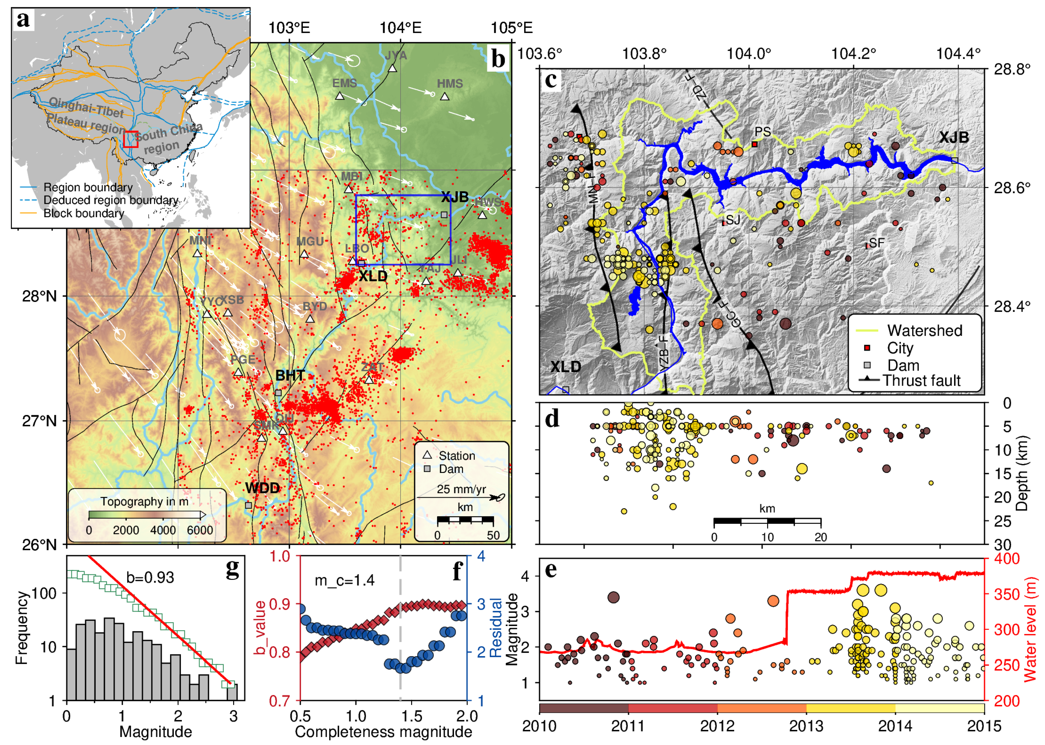
2. Background of the XJB Reservoir

2.1. Geological Settings

Situated downstream of the Jinsha River, the XJB hydropower station is located at the junction of the stable South China block and the Qinghai–Tibet Plateau block (Figure 1a,b). Such a convergence zone indicates strong and varied tectonic activities, such as uplifting, folding and faulting [35]. The NNW–NS striking faults and a few NE striking faults cut the region into segments, resulting in a complex regional tectonic stress environment. Modern GPS measurements [33] reveal a motion velocity field in the region, with speeds ranging from 5 mm/a to 25 mm/a, oriented in a direction from the northwest to the southeast, as a consequence of materials escaping from the Tibetan Plateau towards the southeast [36]. In this grand tectonic context, the NNW–NS striking faults in the region are expected to exhibit both strike-slip and reverse components. The XJB reservoir traverses the north-west trending Mabian–Yanjin fault zone (MYFZ) [37], a tectonic active seismic belt characterized primarily by several thrust faults (e.g., MN-F, YZB-F and GC-F as depicted in Figure 1c. Several $M6.0+$ earthquakes historically occurred in the MYFZ. For instance, an $M7.0$ earthquake in 1216 induced a giant landslide, leading to the creation of Mahu Lake between the YZB-F and the MN-F [38]. Extensive red beds outcrop in the XJB area. In addition, Permian Yanxin limestone is developed in the tail section the XJB reservoir [24,25]. Moreover, two major rivers, namely, the Jinsha River and the Min River, meet at the head of the XJB dam, providing the region with abundant water resources. In addition, due to the significant difference in elevation between the east and west, the river has strong downcutting forces.

2.2. Seismicity and Water Levels

The XJB hydropower plant is the first dam to be constructed among the four cascading conservancy projects on the lower Jinsha River, impounding water to form an approximately 146 km long artificial reservoir. Its first impoundment commenced on 10 October 2012, resulting in a rise in water level by 74 m relative to the average pre-storage elevation of 281 m. No significant surge in seismicity was observed during this period (Figure 1e). During and after reaching the design water lever (i.e., 380 m above sea level), a remarkable increase, some 5–6 times the monthly earthquake count over the ambient seismicity prior to the impoundment, was recorded. Notably, two $M3.0$ earthquakes occurred in August and November 2013, respectively.

3. Methodology

3.1. Seismic Data

Earthquakes in the XJB area from 2010 to 2015 were recorded by the regional and local permanent broadband seismic stations with 100 Hz sampling rate. The frequency–magnitude relation of the original earthquake catalog was estimated after the completeness magnitude ($m_c$) was determined (Figure 1f,g). The seismic b-value (0.93) during the entire period in the XJB reservoir is higher than that of observed in natural cases (0.6–0.8, refer to [39]), which aligns with the typical feature of RIS [5]. To obtain precise results on the spatiotemporal evolution, we used the phase data recorded by the stations within 200 km (Figure 1b) to relocate the events by the double difference location method [40]. The time–space distribution of the relocated seismic catalog is shown in Figure 1c,e. We noticed that the vast majority of events along the reservoir were within the watershed. Several seismic clusters were identified in the tail section of the reservoir between the YZB-F and the MN-F, aligning with the results observed by the reservoir-specific network [26,27]. The epicenters do not exhibit a distinct clustering at depth; however, an interface is discernible at a depth of 5 km (Figure 1d), potentially associated with a regional stratigraphic boundary. We selected the waveform data of $M1.0+$ earthquakes (180 s length for each event) recorded by about 20 seismic stations for the extraction of spectral parameters.

3.2. Data Processing

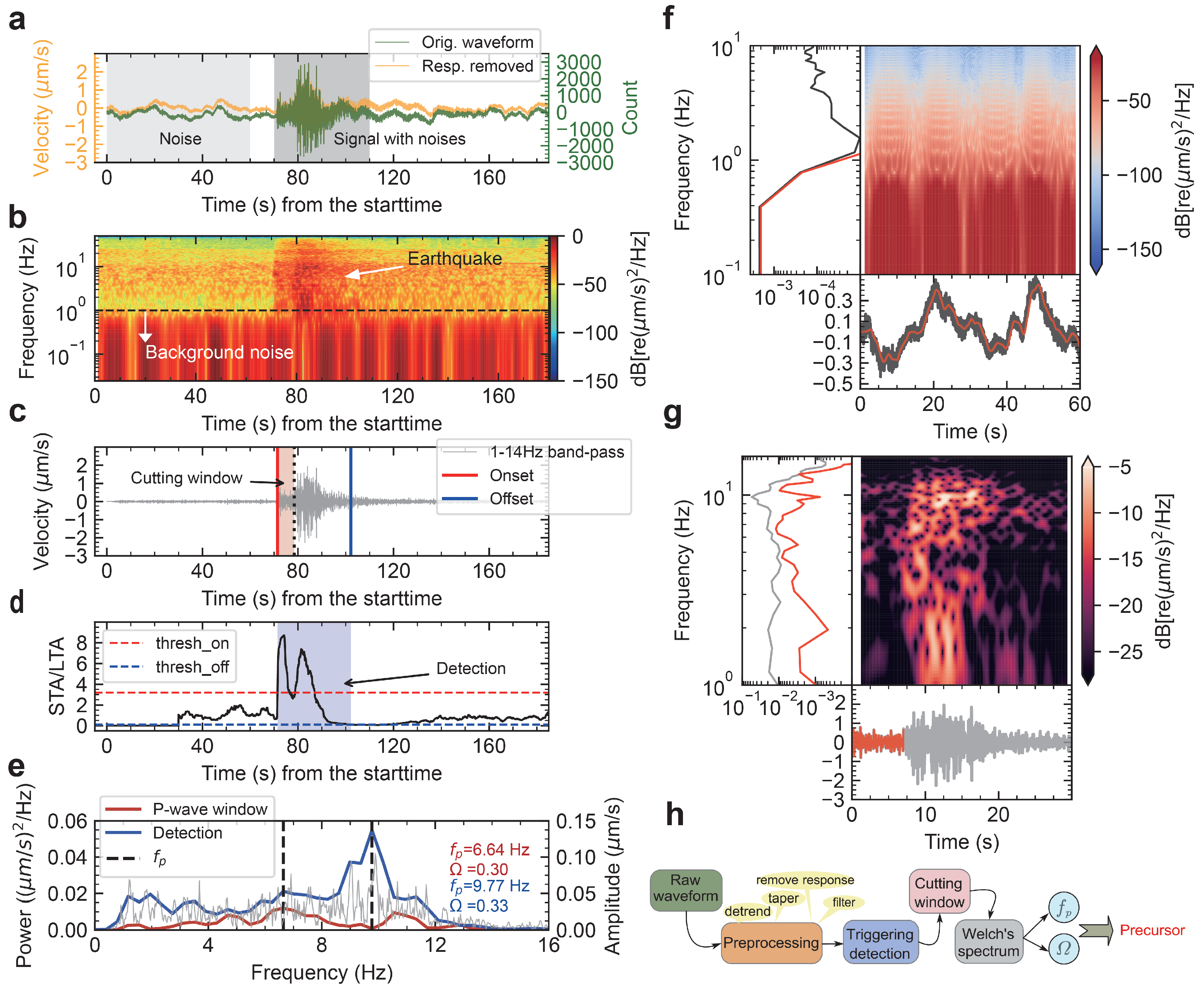
3.2.1. Power Spectra of Earthquakes

To investigate the spectral characteristics of RIS, we need to convert waveform time series to the frequency domain using the Fast Fourier Transform (FFT). The power spectral density (PSD) is computed by averaging the FFT results of individual segments that constitute the entire seismic signal. Thus, the power spectrum is more stable and smoother than the Fourier spectrum for evaluating frequency features of nonstationary seismic signals [41]. In this study, we utilized Welch’s method [42] to obtain power spectra of earthquakes in the XJB reservoir for spectral parameter extraction. Furthermore, a probability density function PSD approach [43] was adopted to visualize power spectra, aiming to identify suitable filtering references during data preprocessing. Taking the LBO station as an example (Figure 2), we can see that the power level of the 2–14 Hz frequency band is relatively low and falls within the range of the new high/low noise models [44]. We used this frequency band range for filtering seismic waveforms to enhance the signal-to-noise ratio, aiding in the detection of P-arrivals.

3.2.2. Spectral Parameters

Parameter analysis (e.g., [45]) proves to be a suitable tool for crack classification when the conventional methods such as moment tensor inversion become ineffective in dealing with low signal-to-noise or low-magnitude events. One well-known example is the rise angle (RA) and the average frequency (AF) ratio method [46], which utilizes characteristic parameters in the time domain to classify cracks and is widely used in acoustic emission monitoring. The author of [28] asserted that observing rupture modes, particularly micro-ruptures, proves challenging in the time domain but is more easily achieved in the frequency domain. His research group (e.g., [20,29,30,45]) introduced a spectral parameter (i.e., peak frequency) approach and devised a statistical strategy for the differentiation of tensile and shear cracks. Recently, a shape factor parameter derived from the frequency domain was successfully employed for the classification of volcanic seismic signals [47]. In addressing the challenge of describing spectral features comprehensively with a single parameter, particularly in the context of predominantly microseismic events in the reservoir area, this study integrates the dominant frequency and the shape factor to explore their spatiotemporal evolution, with the goal of identifying potential precursors associated with RIS.

To explore precursor information related to RIS, we focus on characterizing the P-waves of individual earthquakes, recorded by different stations, through the extraction of spectral parameters, including the peak frequency and the shape factor, from their power spectra. Assume that the P-wave with a certain length has been accurately captured from the event waveform. Its power spectrum, $S\left(f\right)$, is estimated by Welch’s method [42], where $S\left(f\right)$ denotes the amplitude corresponding to the frequency f of the power spectrum. The peak frequency $f_p$ is the frequency at which the spectrum reaches its maximum amplitude, and it can be determined as follows:

$$f_p=argmax\left(S\left(f\right)\right)$$

(1)

where $argmax\left(y\right(x\left)\right)$ denotes the operation of searching the x that maximizes the function $y\left(x\right)$. A series of statistical moments of the power spectrum [47], $m_i$, are computed by the following equations:

$$m_i={\int }_{f_1}^{f2}S\left(f\right)f^{i}df$$

(2)

where for $i=0,1,2$ and $m_i$ represent the zero-, first and second moment, respectively. The upper and lower limits of integration are taken as $f_1=2$ Hz and $f_2=14$ Hz, respectively, according to the filter band in this study. As such, the shape factor of the spectrum, $\Omega$, can be described by the formula:

$$\Omega =\sqrt{1-{\displaystyle \frac{m_1^2}{m_0{m}_2}}}$$

(3)

3.2.3. Data Processing Workflow

In this section, we describe the entire data processing workflow in detail. Taking a vertical component event waveform recorded by the BYD station as an example, after demeaning and tapering the raw waveform, instrument response removal was applied routinely, converting the digital counts to physical velocity (Figure 3a). It is not possible to discern the earthquake signal from the response-removed waveform due to the signal being submerged in noise. The spectrogram (Figure 3b) clearly illustrates that this waveform exhibits a high power level in the frequency band below 2 Hz over time, primarily due to background noise in the region, whereas seismic signals can be observed in the 2–10 Hz frequency band at about 100 s, highlighting the advantage of examining RIS in the frequency domain. We also found that the waveform with frequencies below 2 Hz closely matches the waveform preceding the seismic signal (which we extracted for the first 60 s) (Figure 3f). This implies that we can effectively filter our data with the highpass of 2Hz. To enhance the signal-to-noise for earthquakes, we subsequently applied a bandpass filter ranging from 2 Hz to 14 Hz to the response-removed waveform, as depicted in Figure 3c. After implementing this filtering process, the seismic signal became readily noticeable in the time domain, affirming the suitability of this filter band.

Considering the intricate propagation of seismic waves within the medium and the need to mitigate interference such as refraction and scattering, we refrained from analyzing the entire waveform spectrum. Instead, we focused on extracting the initial arrival wave to obtain the most pristine spectral information from the seismic source. Here, we adopted the short time average/long time average (STA/LTA) technique, a widely used method for detecting signals from recordings [48], to facilitate the detection of P-waves. We selected the appropriate threshold parameters for the SLA/LTA trigger to ensure its applicability to our dataset. As shown in Figure 3c,d, the seismic signal with a start time at 66s and an end time at 120 s was detected. Given our selection of waveforms recorded by stations within a 200 km radius, the maximum travel time difference between the P-wave and S-wave was calculated as 24 s ($200/v_s-200/v_p)=24$. For computational convenience, we cut a 20 s duration for the first arrival wave (the cut window as displayed in Figure 3c). Moreover, the power spectrum of the cut-window waveform was estimated by Welch’s method [42] as described in Section 3.2.1. Finally, the peak frequency $f_p$ and the shape factor $\Omega$ were extracted from the power spectrum using Equations (1)–(3). As shown in Figure 3e, compared to the power spectrum, the Fourier spectrum of the detection, characterized by numerous spikes, lacks smoothness and is thereby not favorable for the extraction of spectral parameters. This is the reason why we employed the power spectrum instead of the Fourier spectrum used in the previous paper [29]. From Figure 3g, we can see that the peak frequency ($f_p=3.91$ Hz shown in Figure 3e) of the detection was identified at 30 s, likely corresponding to the surface wave with maximum amplitude in the time domain. Due to their strong correlation with site effects, surface waves may obscure the inherent characteristics of the seismic source. Therefore, we extracted a cut-window from the entire detection to capture the first arrival body wave, which readily reflects failure patterns of seismic source. The workflow of data processing is depicted in Figure 3h. High values of the shape factor are concentrated in various directions, displaying a narrow distribution. We also observe that the shape factor exhibits more sensitive to distance in the northwest to south direction compared to other directions (see Section 4.1).

4. Results

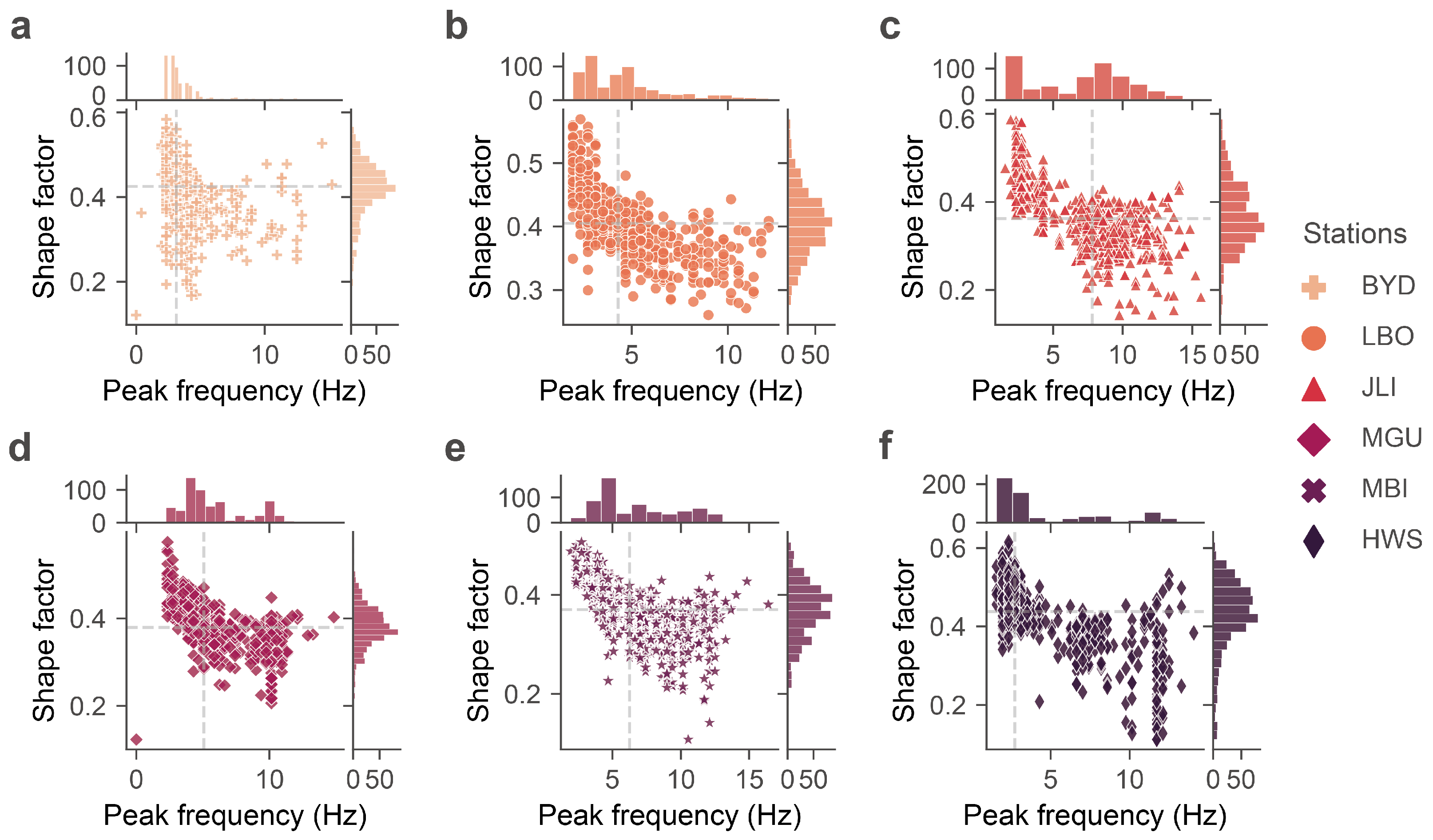
4.1. Joint Distribution of Spectral Parameters and Site Effects

The spectral parameters evaluated by the proposed method introduced in Section 3.2 were obtained for events recorded by the three-component seismometers. For convenience, here we selected six stations within 100 km to display their joint distributions (Figure 4). The results from the six sites reveal analogous joint distributions of the two spectral parameters, albeit with slight differences in the marginal distributions of the peak frequency. The shape factor values predominantly fall within the range of 0.2–0.6, resembling properties of a Gaussian distribution. Peak frequencies are distributed within the filtering range of 2–14 Hz, with the majority concentrated in the lower frequency band of 3–6 Hz. Moreover, it is apparent that the representation of seismicity through the peak frequency and shape factor effectively partitions events into distinct areas of the joint distribution graph (Figure 4), even though the criteria for such classification remain elusive. This study places its emphasis on precursor information rather than the categorization of seismic events. In addition, the variability in the distribution of spectral parameters obtained for stations is influenced by site-specific factors. For instance, station BYD, positioned farthest from the seismic clusters among the six stations (Figure 1b), exhibits a relatively small proportion of the peak frequency in the high-frequency band (>5 Hz), which can be attributed to the rapid attenuation of the high-frequency component.

To examine site effects on the spectral parameters, we analyzed the evolving patterns of the peak frequency and shape factor with respect to the event azimuth and epicentral distance. Using the event coordinates, we computed the epicentral distance and azimuthal angle from each event to its corresponding station. Subsequently, we plotted the relationship between the peak frequency and shape factor of each event against these two independent variables (shown as Figure 5a and Figure 5b), respectively. The peak frequency and shape factor values exhibit non-uniformity across different epicentral distances and azimuths, with specific sites displaying high or low values, thereby empirically confirming the significant impact of the site effects on spectral parameter estimation. To quantitatively characterize such non-uniformity, we conducted data interpolation, and the results are presented in Figure 5d,e. By considering the geometric center of all events within the XJB reservoir as a reference point (Figure 5c), we calculated the distances and azimuth angles of seismic events recorded by different stations relative to this reference point. Then, we applied a radial basis function (RBF) method to interpolate the peak frequency and shape factor dataset within the relative coordinate system. From Figure 5d, we can find that high-peak-frequency events are concentrated in the northwest and southeast directions, with a discernible decreasing trend in the peak frequency as the distance from the reference point increases. The values with higher shape factors are present in various directions except the northeast, forming a narrow and elongated distribution. Notably in the northwest to south direction, the shape factor exhibits greater sensitivity to distance compared to other directions (Figure 5e).

4.2. Temporal Process of Spectral Parameters and the New Indicator

To uncover potential precursors of RIS in the frequency domain, we conducted a statistical analysis of the temporal evolution of spectral parameters. The changes in the peak frequency and shape factor of events throughout the reservoir impoundment process are illustrated in Figure 6c. As we can see, the single event possesses various values due to site effects described in Section 4.1, making it challenging to discern an overall trend in both the peak frequency and shape factor. We calculated three statistical metrics, namely, the mean, the 25th and 75th percentile, for both the peak frequency and shape factor of each event to provide a smoother result of the temporal evolution in spectral parameters. We found that 50% of the events exhibited slight fluctuations over time in the peak frequency within the range of 3–6 Hz and in the shape factor within the range of 0.35–0.46, with their respective mean values converging towards stability at approximately 4 Hz and 0.42 (Figure 6b). Whether before or after reservoir impoundment (Figure 6a), there is no evident inflection point in the temporal evolution of individual spectral parameters.

Based on the results in Figure 4, it is evident that the combination of the two spectral parameters holds the potential to distinguish seismic events. Thus, we introduced a new indicator $k=\Omega /f_p$, defined as the ratio of the shape factor to the peak frequency, and by varying the ratio we can divide the joint distribution graph into different areas. Likewise, the variation in this indicator over time is shown in Figure 6d. It has come to our attention that, as the reservoir impoundment progressed, the majority of events displayed values below 0.25 for this new indicator (k). Prior to impoundment, there were almost no events with k above 0.25. Following the first impoundment (P1 in Figure 6a), a limited number of events exhibited values above 0.25, whereas after the second impoundment (P2 in Figure 6a), a pronounced increase in seismic events with k exceeding 0.25 was observed. This strongly suggests the potential of this indicator as a spectral precursor for RIS.

A comparison of spectral parameters before and after reservoir impoundment is shown in Figure 7. We noticed that the histograms of spectral parameters demonstrate minimal differences before and after reservoir impoundment, with a notably richer distribution of spectral parameters observed after impoundment (Figure 7a–d). The proportion of seismic events with peak frequencies around 7 Hz and around 12 Hz increased following impoundment. The proportion of events with shape factors greater than 0.55 decreased, while the number with shape factors less than 0.2 increased following impoundment. The proportion of events with ratios exceeding 0.25 rose, whereas the number ratios less than 0.02 decreased following impoundment. The distribution of spectral parameters for events recorded by stations within 100 km is more concentrated and narrower than that of events recorded by other stations (Figure 7a), indicating that the estimation of spectral parameters due to the site effect caused by the epicentral distance should not be neglected. Additionally, it is seen that seismic events with k values exceeding 0.25 (blue shading in Figure 7a) are primarily recorded by stations located within a 100 km radius following impoundment. Hence, when utilizing the new indicator as a precursor for RIS, it is advisable to select stations within this 100 km radius for spectral parameter acquisition to mitigate the influence of site effects.

4.3. Spatial Variation in Spectral Parameters

We investigated the spatial variation in the spectral parameters of earthquakes that occurred in the XJB reservoir before and after impoundment. To do so, we selected event waveform data recorded by stations within 100 km to minimize the impact of site effects in spectral parameter estimation. Firstly, we applied our proposed methodology to calculate spectral parameters for all seismic events in the XJB area. Subsequently, we averaged the spectral parameters estimated from the stations within 100 km for each event. Then, we conducted spatial interpolation on the average values of these three spectral parameters. We partitioned the spatial region into a grid with a resolution of $0.05°\times 0.05°$, spanning from longitude $103.55°$ to $104.45°$ and latitude $28.2°$ to $28.8°$. For data interpolation, we employed the Gaussian distance of the radial basis function (RBF) method. Finally, the results before and after impoundment and their difference are depicted in Figure 8.

As depicted in Figure 8, the average spectral parameter values exhibit localized clustering in the spatial domain, which likely reflects differences in seismic rupture patterns due to distinct tectonic structures in the reservoir area. The differences in spectral parameters before and after impoundment primarily vary along both sides of the reservoir, illustrating the impact of water on seismic occurrences. For instance, in the northern segment of the MN-F, the average peak frequency decreased by approximately 2 Hz after impoundment, while it increased by roughly 2 Hz in the central segment. Both the MN-F and YZB-F southern segments experienced an approximately 1.5 Hz increase in the average peak frequency. Additionally, within the step-over between the MN-F and YZB-F, there exists a small area near the reservoir where the average peak frequency decreased by some 2 Hz. After reservoir impoundment, the most pronounced changes in the shape factor are concentrated in the head section of the XJB reservoir. Conversely, in its tail section, the shape factor predominantly displays an increase, with no discernible areas of shape factor reduction. Relative to the pre-impoundment period, the average ratio of the shape factor to the peak frequency shows an increase in different regions along the river valley. Notably, this trend is particularly prominent in the area between the northern ends of the MN-F and YZB-F, where the direction of water flow in the Jinsha River undergoes a 90° shift. According to the results in Figure 6, this ratio can be regarded as a precursor indicator for RIS. Therefore, the regions where this ratio exhibits an increase warranting close monitoring and attention.

5. Discussion

The methodology we developed for extracting spectral parameters offers rapid processing for event waveforms and can be extended to handle continuous waveforms due to its universal seismic detection strategy. Spectral analysis provides a valuable avenue for comprehending seismic sources and uncovering associated precursor information, especially in scenarios where time-domain analysis proves challenging, such as routine monitoring of microseismicity. As our results demonstrate, spectral parameter estimation is susceptible to site-specific influences. Therefore, it is imperative to mitigate site effects as much as possible when assessing spectral parameters, as implemented in this study, involving station selection within a stable radius and spatial-temporal averaging of results. Utilizing our proposed methodology, we conducted a spatiotemporal analysis of seismic spectral parameters for the XJB reservoir, yielding intriguing findings. Nevertheless, there are several points that merit discussion.

Proposing spectral parameters with explicit and physical interpretations is important for our understanding of the seismic process. For instance, the corner frequency of the source spectrum can be used to estimate the stress drop of the source (e.g., [22]). Assuming a circular crack model, Ref. [49] proposed that the crack size L can be estimated from the corner frequency of a P-wave $f_0\left(P\right)$ using

$$L={\displaystyle \frac{C_p{V}_p}{2\pi f_0\left(P\right)}}$$

(4)

where $C_p$ and $V_p$ are the rupture velocity and the P-wave velocity, respectively. Equation (4) indicates that the crack size is inversely proportional to the corner frequency. The results [50] show that the peak frequency is numerically close to the corner frequency. Therefore, we consider that the peak frequency, one spectral parameter estimated in this study, can to some extent reflect the source dimension (or crack size). In this study, we opted for the peak frequency as the spectral parameter instead of the corner frequency for two main reasons. Firstly, peak frequency extraction is more straightforward and time-efficient compared to the corner frequency, which necessitates fitting methods. Secondly, we aimed to facilitate the comparison between regional-scale (this study) and laboratory-scale results [20,29], as the laboratory findings are based on peak frequency estimation. Our results display an increase in high-peak-frequency events in the XJB reservoir after impoundment (Figure 6c and Figure 7b). These events are associated with smaller crack sizes (Equation (4)), indicating that the rise in microseismicity around the reservoir following impoundment driven by water diffusion [51], which aligns with the monitoring results (Figure 1e). In terms of spatial distribution, a concentrated area of high-peak-frequency events is observed in the step-over between the YZB-F and the MN-F (Figure 8d) after reservoir impoundment, which [24,25] suggested is associated with karst collapses due to the presence of limestone formations. Hence, estimating the peak frequency provides a novel opportunity for monitoring and predicting RIS associated with karst collapses in the reservoir area. Another parameter, the shape factor, is defined geometrically by moments and describes the shape of the spectrum but lacks an explicit physical interpretation. Combining these two parameters allows for a comprehensive characterization of spectral features and the discovery of seismic precursors related to reservoir impoundment (Figure 6d).

The selection of the filtering bandwidth also exerts an influence on the estimation outcomes of spectral parameters. Depending on diverse application scenarios and the sampling frequencies of the stations, it is essential to select an appropriate filtering range. This step enhances the efficacy of our developed method in extracting spectral parameters. In this study, to compensate for the lack of filtering process before converting the time-domain signals into frequency-domain signals in previous studies [20,28,29], we used a relatively narrow bandwidth (2–14 Hz) for detecting the P-wave window signal for the reasons listed in Section 3.2.1. A wide bandwidth (2–40 Hz) was utilized for filtering the volcanic seismic signals to extract spectral parameters [47]. To evaluate the influence of various filtering bandwidths on our research outcomes, we also employed a wider bandwidth of 1–40 Hz. The outcomes from this filtering process differed in terms of the spectral parameter ranges ($f_p\in (1,40),\Omega \in (0.1,0.9)$) compared to our study’s results, but the overall distribution of spectral parameters remained largely consistent. In addition, the critical point for identifying RIS precursors (k) was estimated to be 0.37, which is higher than the 0.15 obtained in this study. The filtering bandwidth can be determined by estimating the PSD probability density function of all earthquakes in the region as we did in this study (Figure 2).

In comparison to laboratory-scale acoustic emission tests conducted during rock failure, the seismic signals associated with regional-scale ruptures did not exhibit the expected twin-peak frequency distribution [20,28,29]. We attribute this difference to two factors: (1) Unlike laboratory tests with single loading modes like tension, shear and compression, regional-scale external loading conditions are diverse and complex, influenced by factors such as tectonic stress, faults and external elements (e.g., reservoir impoundment); (2) At the regional scale, the geological medium, especially after reservoir impoundment, exhibits greater heterogeneity than laboratory rock samples, leading to intricate elastic wave propagation influenced by dispersion effects. In addition, Refs. [29,46] classified rock fracture types based on time-domain and frequency-domain parameters, respectively, building upon known macroscopic failure experiments. On the other hand, categorized volcanic event types using frequency-domain parameters [47], also in cases where event types were known in advance. However, this study proposed a precursor indicator for identifying RIS based on parameter analysis, as we did not have prior knowledge of event types. Therefore, in the future, we can use the threshold of this new indicator to select those events associated with RIS for in-depth analysis (such as moment tensor inversion) to reveal the mechanisms behind RIS.

6. Conclusions

We developed a spectral parameter extraction method applicable to reservoir-induced seismicity (RIS) and performed a spatiotemporal analysis of spectral parameters, including the peak frequency and shape factor, for earthquakes in the XJB reservoir area from 2010 to 2015. This study provides insights into potential RIS precursors and contributes to RIS monitoring and risk management. Our main findings are highlighted as follows:

(1)

The power spectral characteristics of earthquakes in the XJB reservoir area can be effectively captured using two spectral parameters, the peak frequency and shape factor. The shape factor follows a normal distribution within the 0.2–0.6 range, while the peak frequency spans 2–14 Hz, with the highest proportion observed in the lower frequency band of 2–6 Hz.

(2)

The estimation of spectral parameters is influenced by site-specific factors. The peak frequency is particularly sensitive to azimuthal angles, whereas the shape factor is more responsive to epicentral distances.

(3)

There are minimal discrepancies in the distribution of spectral parameters before and after reservoir impoundment. Post-impoundment, there is a slight increase in the proportion of high peak frequencies, correlating with a higher occurrence of microseismic events. Temporal analysis shows no significant shifts in individual parameters in response to water level changes. However, a notable increase in the ratio (k) of the shape factor to the peak frequency after reservoir impoundment suggests its potential as a precursor indicator for RIS.

(4)

Spatial variations in spectral parameters reflect differences in the seismogenic structure within the reservoir area and the effects of reservoir water on seismic sources. Particularly, several regions between the two faults in the tail section of the XJB reservoir exhibit an increase ratio (k) of the shape factor to the peak frequency after impoundment, indicating that these areas require close monitoring for future RIS study.

In the future, we will collect data from additional artificial water reservoirs and more recent sources to further evaluate the general applicability of our spectral precursor indicator and to implement the proposed method in practical engineering scenarios.

References

1. Sayão, E.; França, G.S.; Holanda, M.; Gonçalves, A. Spatial database and website for reservoir-triggered seismicity in Brazil. Nat. Hazards Earth Syst. Sci. 2020, 20, 2001–2019. [Google Scholar] [CrossRef]
2. Shen, Y.; Liu, D.; Jiang, L.; Nielsen, K.; Yin, J.; Liu, J.; Bauer-Gottwein, P. High-resolution water level and storage variation datasets for 338 reservoirs in China during 2010–2021. Earth Syst. Sci. Data 2022, 14, 5671–5694. [Google Scholar] [CrossRef]
3. Năstase, G.; Şerban, A.; Năstase, A.F.; Dragomir, G.; Brezeanu, A.I.; Iordan, N.F. Hydropower development in Romania. A review from its beginnings to the present. Renew. Sustain. Energy Rev. 2017, 80, 297–312. [Google Scholar] [CrossRef]
4. Ge, S.; Liu, M.; Lu, N.; Godt, J.W.; Luo, G. Did the Zipingpu Reservoir trigger the 2008 Wenchuan earthquake? Geophys. Res. Lett. 2009, 36, L20315. [Google Scholar] [CrossRef]
5. Gupta, H.K. Artificial water reservoir-triggered seismicity (RTS): Most prominent anthropogenic seismicity. Surv. Geophys. 2022, 43, 619–659. [Google Scholar] [CrossRef]
6. Gahalaut, K. On the Common Features of Reservoir Water-Level Variations and Their Influence on Earthquake Triggering: An Inherency of Physical Mechanism of Reservoir-Triggered Seismicity. Bull. Seismol. Soc. Am. 2021, 111, 2720–2732. [Google Scholar] [CrossRef]
7. Carder, D.S. Seismic investigations in the Boulder Dam area, 1940-1944, and the influence of reservoir loading on local earthquake activity. Bull. Seismol. Soc. Am. 1945, 35, 175–192. [Google Scholar] [CrossRef]
8. Wilson, M.; Foulger, G.; Gluyas, J.; Davies, R.; Julian, B. HiQuake: The human-induced earthquake database. Seismol. Res. Lett. 2017, 88, 1560–1565. [Google Scholar] [CrossRef]
9. Gupta, H.K. Reservoir triggered seismicity (RTS) at Koyna, India, over the past 50 yrs. Bull. Seismol. Soc. Am. 2018, 108, 2907–2918. [Google Scholar] [CrossRef]
10. Michas, G.; Pavlou, K.; Vallianatos, F.; Drakatos, G. Correlation between seismicity and water level fluctuations in the Polyphyto Dam, North Greece. Pure Appl. Geophys. 2020, 177, 3851–3870. [Google Scholar] [CrossRef]
11. Dong, S.; Li, L.; Zhao, L.; Shen, X.; Wang, W.; Huang, H.; Peng, B.; Xu, X.; Gao, R. Seismic evidence for fluid-driven pore pressure increase and its links with induced seismicity in the Xinfengjiang Reservoir, South China. J. Geophys. Res. Solid Earth 2022, 127, e2021JB023548. [Google Scholar] [CrossRef]
12. Yan, Z.L.; Qin, L.L.; Wang, R.; Li, J.; Wang, X.M.; Tang, X.L.; An, R.D. The application of a multi-beam echo-sounder in the analysis of the sedimentation situation of a large reservoir after an earthquake. Water 2018, 10, 557. [Google Scholar] [CrossRef]
13. Chen, Y.; Nakatsugawa, M.; Ohashi, H. Research of impacts of the 2018 Hokkaido Eastern Iburi Earthquake on sediment transport in the Atsuma River basin using the SWAT model. Water 2021, 13, 356. [Google Scholar] [CrossRef]
14. Zhang, M.; Ge, S.; Yang, Q.; Ma, X. Impoundment-associated hydro-mechanical changes and regional seismicity near the Xiluodu reservoir, Southwestern China. J. Geophys. Res. Solid Earth 2021, 126, e2020JB021590. [Google Scholar] [CrossRef]
15. Do Nascimento, A.F.; Cowie, P.; Lunn, R.; Pearce, R. spatio-temporal evolution of induced seismicity at Açu reservoir, NE Brazil. Geophys. J. Int. 2004, 158, 1041–1052. [Google Scholar] [CrossRef]
16. Zhang, L.; Lei, X.; Liao, W.; Li, J.; Yao, Y. Statistical parameters of seismicity induced by the impoundment of the Three Gorges Reservoir, Central China. Tectonophysics 2019, 751, 13–22. [Google Scholar] [CrossRef]
17. Li, L.; Luo, G. What causes the spatiotemporal patterns of seismicity in the Three Gorges Reservoir area, central China? Earth Planet. Sci. Lett. 2022, 592, 117618. [Google Scholar] [CrossRef]
18. Fu, Z.; Chen, F.; Deng, J.; Zhao, S.; Li, H.; Dai, S.; Shao, Y.; Fu, Y.; Zhu, J.; Cheng, W. Statistical investigation of induced seismicity associated with the impoundment of the Xiangjiaba Reservoir, Southwestern China. Bull. Eng. Geol. Environ. 2024, 83, 106. [Google Scholar] [CrossRef]
19. Telesca, L. Analysis of the cross-correlation between seismicity and water level in the Koyna area of India. Bull. Seismol. Soc. Am. 2010, 100, 2317–2321. [Google Scholar] [CrossRef]
20. Zhu, J.; Deng, J.; Chen, F.; Wang, F. Failure analysis of water-bearing rock under direct tension using acoustic emission. Eng. Geol. 2022, 299, 106541. [Google Scholar] [CrossRef]
21. Hua, W.; Zheng, S.; Yan, C.; Chen, Z. Attenuation, site effects, and source parameters in the Three Gorges Reservoir area, China. Bull. Seismol. Soc. Am. 2013, 103, 371–382. [Google Scholar] [CrossRef]
22. Mahato, C.; Shashidhar, D. Stress drop variations of triggered earthquakes at Koyna–Warna, western India: A case study. J. Earth Syst. Sci. 2022, 131, 106. [Google Scholar] [CrossRef]
23. Shi, J.; Zhao, C.; Yang, Z.; Xu, L. Study on Seismic Source Parameter Characteristics of Baihetan Reservoir Area in the Lower Reaches of the Jinsha River. Water 2024, 16, 1370. [Google Scholar] [CrossRef]
24. Feng, X.; Yue, X.; Wang, Y.; Wang, X.; Diao, G.; Zhang, H.; Cheng, W.; Li, Y.; Feng, Z. Discussion on genesis of induced earthquake based on focal mechanism in Xiangjiaba reservoir region. Seismol. Geol. 2015, 37, 565–575. [Google Scholar]
25. Feng, Z.; Cheng, W.; Diao, G.; Zhang, H.; Li, W. Seismicity of the Xiangjiaba reservoir after impoundment. Earthq. Res. China 2015, 31, 319–328. [Google Scholar]
26. Zhao, C.; Zhao, C.; Lei, H.; Yao, M. Seismic activities before and after the impoundment of the Xiangjiaba and Xiluodu reservoirs in the lower Jinsha River. Earthq. Sci. 2022, 35, 355–370. [Google Scholar] [CrossRef]
27. Yang, L.; Li, B.; Chang, T. Seismicity characteristics of Xiangjiaba Reservoir region before and after the impoundment. J. Geod. Geodyn. 2019, 39, 919–923. [Google Scholar]
28. Deng, J.; Li, L.; Chen, F.; Liu, J.; Yu, J. Twin-peak frequencies of acoustic emission due to the fracture of marble and their possible mechanism. Adv. Eng. Sci. 2018, 50, 1–6. [Google Scholar]
29. Li, L.; Deng, J.; Zheng, L.; Liu, J. Dominant frequency characteristics of acoustic emissions in white marble during direct tensile tests. Rock Mech. Rock Eng. 2017, 50, 1337–1346. [Google Scholar] [CrossRef]
30. Zhu, J.; Deng, J.; Pak, R.Y.; Liu, J.; Lyu, C. Experimental study on the failure process of water-bearing rock under uniaxial tension based on dominant frequency analysis of acoustic emission. Bull. Eng. Geol. Environ. 2023, 82, 233. [Google Scholar] [CrossRef]
31. Clarke, J.; Adam, L.; Sarout, J.; van Wijk, K.; Kennedy, B.; Dautriat, J. The relation between viscosity and acoustic emissions as a laboratory analogue for volcano seismicity. Geology 2019, 47, 499–503. [Google Scholar] [CrossRef]
32. Zhang, G.; Ma, H.; Wang, H.; Wang, X. Boundaries between active-tectonic blocks and strong earthquakes in the China mainland. Chin. J. Geophys. 2005, 48, 602–610. [Google Scholar] [CrossRef]
33. Wang, M.; Shen, Z.K. Present-day crustal deformation of continental China derived from GPS and its tectonic implications. J. Geophys. Res. Solid Earth 2020, 125, e2019JB018774. [Google Scholar] [CrossRef]
34. Deng, Q. Active tectonics and earthquake activities in China. Earth Sci. Front. 2003, 10, 66. (In Chinese) [Google Scholar]
35. Xu, X.; Chen, G.; Wang, Q.; Chen, L.; Ren, Z.; Xu, C.; Wei, Z.; Lu, R.; Tan, X.; Dong, S.; et al. Discussion on seismogenic structure of Jiuzhaigou earthquake and its implication for current strain state in the southeastern Qinghai-Tibet Plateau. Chin. J. Geophys. 2017, 60, 4018–4026. [Google Scholar]
36. Royden, L.H.; Burchfiel, B.C.; King, R.W.; Wang, E.; Chen, Z.; Shen, F.; Liu, Y. Surface deformation and lower crustal flow in eastern Tibet. Science 1997, 276, 788–790. [Google Scholar] [CrossRef] [PubMed]
37. Zhang, S.; Nie, G.; Liu, X.; Ren, J.; Su, G. Kinematical and structural patterns of Yingjing-Mabian-Yanjin fault zone, southeast of Tibetan Plateau, and its segmentation from earthquakes. Seismol. Geol. 2005, 27, 221–233. [Google Scholar]
38. Cui, Y.; Deng, J.; Hu, W.; Xu, C.; Ge, H.; Zheng, J. 36Cl exposure dating of the Mahu Giant landslide (Sichuan Province, China). Eng. Geol. 2021, 285, 106039. [Google Scholar] [CrossRef]
39. Yao, Y.; Wang, Q.; Liao, W.; Zhang, L.; Chen, J.; Li, J.; Yuan, L.; Zhao, Y. Influences of the Three Gorges Project on seismic activities in the reservoir area. Sci. Bull. 2017, 62, 1089–1098. [Google Scholar] [CrossRef]
40. Waldhauser, F.; Ellsworth, W. A double-difference earthquake location algorithm: Method and application to the Northern Hayward Fault, California. Bull. Seismol. Soc. Am. 2000, 90, 1353–1368. [Google Scholar] [CrossRef]
41. Anthony, R.E.; Ringler, A.T.; Wilson, D.C.; Bahavar, M.; Koper, K.D. How processing methodologies can distort and bias power spectral density estimates of seismic background noise. Seismol. Res. Lett. 2020, 91, 1694–1706. [Google Scholar] [CrossRef]
42. Welch, P. The use of fast Fourier transform for the estimation of power spectra: A method based on time averaging over short, modified periodograms. IEEE Trans. Audio Electroacoust. 1967, 15, 70–73. [Google Scholar] [CrossRef]
43. McNamara, D.E.; Buland, R.P. Ambient noise levels in the continental United States. Bull. Seismol. Soc. Am. 2004, 94, 1517–1527. [Google Scholar] [CrossRef]
44. Peterson, J.R. Observations and Modeling of Seismic Background Noise; US Geological Survey: Reston, VA, USA, 1993; Volume 93. [Google Scholar]
45. Zhang, Z.; Deng, J. A new method for determining the crack classification criterion in acoustic emission parameter analysis. Int. J. Rock Mech. Min. Sci. 2020, 130, 104323. [Google Scholar] [CrossRef]
46. Ohno, K.; Ohtsu, M. Crack classification in concrete based on acoustic emission. Constr. Build. Mater. 2010, 24, 2339–2346. [Google Scholar] [CrossRef]
47. Galluzzo, D.; Nardone, L.; La Rocca, M.; Esposito, A.M.; Manzo, R.; Di Maio, R. Statistical moments of power spectrum: A fast tool for the classification of seismic events recorded on volcanoes. Adv. Geosci. 2020, 52, 67–74. [Google Scholar] [CrossRef]
48. Allen, R.V. Automatic earthquake recognition and timing from single traces. Bull. Seismol. Soc. Am. 1978, 68, 1521–1532. [Google Scholar] [CrossRef]
49. Sato, T.; Hirasawa, T. Body wave spectra from propagating shear cracks. J. Phys. Earth 1973, 21, 415–431. [Google Scholar] [CrossRef]
50. Sueyoshi, K.; Kitamura, M.; Lei, X.; Katayama, I. Identification of fracturing behavior in thermally cracked granite using the frequency spectral characteristics of acoustic emission. J. Mineral. Petrol. Sci. 2023, 118, 221014. [Google Scholar] [CrossRef]
51. Yin, G.; Zhang, H.; Shi, Y. Cascade effects of triggered earthquakes of cascade dams: Taking Xiluodu and Xiangjiaba reservoirs as examples. Chin. J. Geophys. 2023, 66, 2470–2488. [Google Scholar]
Figure 1. Tectonic context and seismicity from 2010 to 2015 in the XJB area. (a) Active blocks in Chinese mainland. Red rectangle indicates the extent of (b). Block boundary data refer to [32]. (b) Modern GPS velocity field, active faults, main rivers, earthquake epicenters and location of the four cascading artificial dams in the lower Jinsha River. Earthquakes plotted in red dots are sourced from the China Earthquake Data Center (https://data.earthquake.cn/, last accessed on 2 August 2024). The GPS data are available in [33], and the error ellipse in the legend represents 70% confidence. The digitized fault data originate from [34]. Only seismic stations within a 200 km radius of the blue rectangle, which represents the extent of (c), are mapped. (c) Distribution of relocated earthquakes that occurred in the XJB reservoir. (d) Focal depth along the longitude axis of (c). (e) Temporal process of earthquake magnitude and water level variations in the XJB reservoir. Panels (f,g) present the estimation of completeness magnitude and the frequency–magnitude relation in the XJB area, respectively.
Water 16 02217 g001
Figure 2. PSD probability density function estimated using vertical component waveform data of relocated earthquakes recorded by the LBO station (shown in Figure 1b) from 2010 to 2015 in the XJB reservoir area. We selected approximately 270 event waveforms to calculate the PSD probability density function. Each waveform, sampled at 100 Hz, has a duration of 180 s. We used 128 samples to perform the FFT of each PSD and then estimated the probabilities of each frequency by collecting all PSDs. For more computational details, please refer to [43]. NLNM/NHNM (dashed gray lines) denotes the new low/high noise model [44].
Water 16 02217 g002
Figure 3. Data processing workflow using a vertical component event waveform recorded by the BYD station in October 2011 as an example. (a) The original event waveform (yellow curve) with 180 s length and its instrument response removed version (green curve) after the demeaning and tapering operations. (b) The spectrogram of the response removed waveform. (c) A 2–14 Hz bandpass filter applied to the green curve in (a). Red and blue vertical lines in (c) indicate the starttime and the endtime of the detection identified using the short time average/long time average (STA/LTA) technique [48], respectively. The cut-window (red shaded area in (c) was set to 20 s in this study. (d) The characteristic function of the STA/LTA trigger with respect to the waveform in (c). Red and blue dotted lines signify the thresholds we assigned to detect the earthquake. (e) Power spectra [42] of the cut-window waveform and the detection as well as their spectral parameters. Gray curve indicates the Fourier spectrum of the detection. (f,g) are spectrograms of the waveform (green curve in (a)) with frequencies below 2 Hz and the detection, respectively. Gray curves in (f) indicate the first 60 s of data before the seismic signal. Red curves in (g) indicate the cut-window data. (h) Flowchart of the data processing.
Water 16 02217 g003
Figure 4. Joint distribution of the peak frequency and shape factor estimated for the (a) BYD, (b) LBO, (c) JLI, (d) MGU, (e) MBI and (f) HWS stations within 100 km of the epicenter. Each data point represents the corresponding event recorded by the three-component stations, distinguished by various symbols. The top and right subplots of each panel display the marginal distributions of X and Y in counts. Gray dotted lines in each panel indicate the medians.
Water 16 02217 g004
Figure 5. Site effects of spectral parameters in the XJB area. Distribution of peak frequency (a) and shape factor (b) for events recorded by distinct stations in a polar coordinate system consisting of azimuth and epicentral distance. Markers with varying symbols and colors represent events recorded by their corresponding stations and the values of their spectral parameters, respectively. (c) Earthquakes (black crosses) recorded by the stations (red triangles) within a 100 km radius of the XJB reservoir, using relative coordinates with the geometric center of all events coordinates as the reference point. Interpolation results for peak frequency (d) and shape factor (e) in (c), achieved through the radial basis function (RBF) method.
Water 16 02217 g005
Figure 6. Temporal process of spectral parameters. (a) Water levels of the XJB reservoir and histogram of earthquake occurrence rate in counts per month. P1, P2 and P3 denote the three impoundment periods [24]. (b) The three statistics for the peak frequency (blue color) and shape factor (yellow color), namely, the mean (solid curve), 25th and 75th percentile (the lower and upper boundaries of the shadow), evolve over time. (c) Scatter plot of the two spectral parameters of events recorded by six stations versus time. (d) The ratio of the shape factor to the peak frequency evolves over time. The critical point signifies a significant increase in seismic events with the ratio exceeding 0.25 following the second impoundment.
Water 16 02217 g006
Figure 7. Comparison of spectral parameters before and after reservoir impoundment. (a) Shape factor versus peak frequency for all used stations. Shaded symbols represent post-impoundment events, while unshaded symbols represent pre-impoundment ones. Stacked histograms of f p (b), Ω (c) and k (d) before and after reservoir impoundment.
Water 16 02217 g007
Figure 8. Spatial distribution of spectral parameters in the XJB area. The average peak frequency ( f p ), average shape factor ( Ω ) and their ratio (k) before impoundment are presented in (a), (b) and (c), respectively. These parameters after impoundment are shown in (d), (e) and (f), respectively. The differences ( Δ f p , Δ Ω and Δ k , after minus before) are illustrated in (g), (h) and (i), respectively.
Water 16 02217 g008
Disclaimer/Publisher’s Note: The statements, opinions and data contained in all publications are solely those of the individual author(s) and contributor(s) and not of MDPI and/or the editor(s). MDPI and/or the editor(s) disclaim responsibility for any injury to people or property resulting from any ideas, methods, instructions or products referred to in the content.