Enhancing Water Management: A Comparative Analysis of Time Series Prediction Models for Distributed Water Flow in Supply Networks

Abstract

Water scarcity poses a significant challenge to social integration and economic development, necessitating efficient water management strategies. This study compares time series forecasting models, both classical, Holt–Winters and ARIMA, and modern, LSTM and Prophet, to determine the most accurate model for predicting water flow in public supply networks. Data from four rural Portuguese locations were used, with preprocessing ensuring quality and uniformity. Performance metrics were evaluated for both medium-term (10 days) and long-term (3 months) forecasts. Results indicate that classical models like Holt–Winters and ARIMA perform better for medium-term predictions, while modern models, particularly LSTM, excel in long-term forecasts by effectively capturing seasonal patterns. Future research should integrate additional variables and explore hybrid models to enhance forecasting accuracy.

1. Introduction

Water scarcity represents a significant constraint regarding social integration and economic development. While agriculture accounts for 80% of water usage, domestic demand is also rising due to population growth, lifestyle changes, and global warming. These factors are decreasing water availability and increasing demand, necessitating better planning for water reserves, recycling, and efficient use, as well as real-time monitoring systems [1].

Enhancing water distribution efficiency requires pro-active management based on consumption forecasting, rather than reactive management based on current consumption. Accurate forecasting can reduce operating costs by approximately 18% [2], underscoring the importance of selecting the right model for specific dataset characteristics.

There is a considerable body of research work that deals with time series forecasting for water demand [3,4,5,6]. However, most of these studies use time series data from urban areas or, if focusing on rural areas, they correspond to a large number of users within the water distribution systems [7]. Moreover, many authors direct their forecasts towards short-term periods (hourly, daily, or time steps less than a week). On the other hand, forecasting for the medium term (weekly to monthly) or long term (longer than a month) has not yet been fully explored. Medium- and long-term demand forecasting are important for planning and design of water supply systems, managing water resources, and maintenance activities [8].

This work focuses primarily on monitoring of water flow rates in distribution networks in rural areas characterized by low populational density and water scarcity. It aims to forecast the medium- and long-term water demand in rural areas using both classical and modern forecasting methods. Among the classical models, two statistical approaches were considered: the simpler Holt–Winters models and the more advanced AutoRegressive Integrated Moving Average (ARIMA). The modern methods used are the Long-Short-Term Memory (LSTM), a type of deep learning neural network that has gained wide popularity in time series prediction, and Prophet, a recent regression forecasting model that has been successfully used in several time series forecasting tasks, but not yet explored enough in water demand forecasting.

This paper is organized as follows: Section 2—Selected Models and Related Research provides an overview of the research field and of the characteristics of the models used; Section 3—Materials and Methods describes the datasets, the pre-processing and analysis steps, and the model parameter definitions; and Section 4—Results presents the forecasting results for the different time series. The discussion of the results and the conclusions are presented in Section 5—Discussion and Section 6—Conclusions, respectively.

2. Selected Models and Related Research

Holt–Winters and ARIMA are examples of parametric or statistical models, because they require knowledge of the distribution characteristics of the time series. The three main characteristics of a time series are trend, seasonality, and residuals. The trend, which can be increasing or decreasing, may take on a wide variety of patterns such as linear, exponential, dampened, and polynomial. Seasonality refers to cyclic patterns that repeat at constant time intervals. Residuals are short-term fluctuations that are neither systematic nor predictable [3].

The Holt–Winters model is a well-regarded forecasting method for time series data that exhibit both trend and seasonality. It extends the simple exponential smoothing model by incorporating two additional smoothing equations: one for the trend component and one for the seasonal component. The model comes in two variations, additive and multiplicative, chosen based on whether the seasonal variations are roughly constant or proportional to the level of the series. The Holt–Winters method is particularly effective for short-term forecasting, as it dynamically updates the level, trend, and seasonal components to adapt to changes in the data. By smoothing these components separately, the model provides a comprehensive approach to capturing the underlying patterns in time series data, making it suitable for various practical applications in forecasting.

The ARIMA algorithm combines three components: autoregressive (AR), differencing (I for integrated), and moving average (MA). The AR part involves regressing the variable on its own lagged values, the I part involves differencing the data to achieve stationarity, and the MA part models the error term as a linear combination of error terms occurring contemporaneously and at various times in the past. The parameters (p, d, q) of the ARIMA model represent the order of the autoregressive part, the degree of differencing, and the order of the moving average part, respectively. This algorithm is particularly effective for short-term forecasting due to its ability to capture various types of temporal structures in time series data.

Classical time series forecasting models like ARIMA and Holt–Winters have been extensively used in various domains [3,9]. For instance, a study comparing ARIMA and Holt–Winters models for COVID-19 forecasting in India over a 20-day time horizon found that ARIMA achieved over 99% accuracy, outperforming Holt–Winters [9]. These results highlight ARIMA’s strength in short-term predictions, particularly when dealing with datasets exhibiting clear trends and seasonality.

Machine learning involves non-parametric models that do not require a prior knowledge about the characteristics of the datasets. These methods demonstrate good performance even in cases where time series exhibit non-linear behaviors. Examples of such methods include Support Vector Regression, k-Nearest Neighbor, and Artificial Neural Networks [5,10]. In recent years, machine learning algorithms in the field of deep learning networks have grown in popularity. Among these, the Long-Short-Term Memory (LSTM) neural networks have achieved excellent performance in several forecasting tasks [11,12].

LSTM is a type of recurrent neural network that is well suited for time series forecasting due to its ability to capture long-term dependencies in sequential data. Unlike traditional RNNs, LSTMs are designed to avoid the problem of an exploding/vanishing gradient that arises in long-term dependencies. It uses a set of gates (input, forget, and output gates) to control the flow of information. These gates allow the LSTM to retain or discard information over long periods, making it highly effective for tasks where past information is crucial for predicting future values. The architecture includes memory cells that store information, and these cells are updated by the gates based on the input data and previous cell states. This design enables LSTM models to perform exceptionally well in capturing trends and seasonality in time series data, making them a powerful tool for forecasting applications [13,14]. It is worth noting that, when applied to time series, LSTM models can be further classified as univariate, if only a single time series is used, or multivariate, which incorporates multiple variables to enhance predictive accuracy.

LSTM models have shown promise in improving time series forecasts in different fields [15,16]. In a study conducted in Yazd, Iran, a univariate and a multivariate LSTM model were compared to predict monthly water consumption based on climate effects [13], where the multivariate model included monthly air temperature values besides water consumption values. The results showed that the multivariate model had lower prediction errors.

Similarly, LSTM models have proven to be effective for next-day water consumption predictions to optimize pumping systems, showing superiority over autoregressive models [17]. When comparing the effectiveness of the classic ARIMA model with the LSTM model applied to a time series of financial index values, a substantial reduction in the error metric is observed with the LSTM model, thus indicating a much higher performance of the LSTM compared to ARIMA [18].

The Prophet model is a relatively new regression forecasting model developed by researchers form Facebook [19]. This model was designed to handle time series data with strong seasonal effects and missing data points. It is particularly well suited for time series data that display daily, weekly, and yearly seasonality patterns. Prophet uses an additive model to decompose the time series into trend, seasonality, and holidays, as expressed in the following equation:

$$y_t=g_t+s_t+h_t+{\epsilon }_t$$

where $y_t$ is the predicted value, $h_t$ is the trend, $s_t$ is the seasonality, $h_t$ is the holiday effect, and ${\epsilon }_t$ is the error associated with each time step t. The trend can be modelled as a linear function or as a non-linear function called saturation growth (Equation (1)).

$$g_t=\frac{C}{1+\exp (-\left(k+a_t\delta \right)(t-\left(m+a_t\delta \right))}$$

(1)

where C is the carrying capacity, k is the growth rate, m is an offset parameter, a is a binary value indicating the presence of the effect from change point t, and $\delta$ is the rate change adjustment.

The seasonality is modelled using a standard Fourier series, as in Equation (2),

$$s_t={\sum }_{i=1}^N\left(a_i\cos \left(\frac{2\pi it}{P}\right)+b_i\sin \left(\frac{2\pi it}{P}\right)\right)$$

(2)

where P is the regular period the series is expected to have, and N is automatically selected for the different periods. The holiday term is incorporated in the model as a list of holidays.

Unlike traditional models, Prophet is resilient to missing data and shifts in the trend, making it highly effective for real-world forecasting scenarios.

In the original publication, the Prophet model is used to forecast the number of events created on Facebook by its users, and outperforms traditional models such as ARIMA, exponential smoothing, and Random Walk. Prophet has since been used in a variety of forecasting applications, such as in oil production [20], energy demand [21], and healthcare [22]. However, reports on the use of the Prophet model for forecasting water demand are scarce [23]. To our knowledge, it has not yet been applied for medium- or long-term water demand forecasting.

A comparison of ARIMA, LSTM, and Prophet models applied to oil production time series showed that the ARIMA and LSTM models outperformed Prophet. However, Prophet uniquely captured winter fluctuations [20]. In the healthcare sector, a comparison of ARIMA and Prophet models showed that Prophet generally outperformed ARIMA [22]. However, ARIMA performed better when strong seasonal patterns were absent. Additionally, Prophet was less reliable in handling data with many outliers due to measurement errors.

One of the important aspects of forecasting is the horizon of the predictions: short-term forecast (less than a week), medium-term forecast (week to month), and long-term forecast (more than a month) [8]. Most of the research works focus on short-term water consumption predictions. In [24], forecasts are made for the next hour; in [17], the aim is to predict the following day’s water consumption as a global value; and in [25], hourly forecasts are made. Few studies aim to provide forecasts in the medium and long term [13,26]. Frequently, climatic factors such as air temperature were used alongside the distributed flow data as additional training information [8].

The present study focuses on hourly predictions for both medium-term (ten days) and long-term (three months) forecasts. Due to the difficulty in obtaining reliable climatic forecasts for these time horizons, the predictions are solely based on historical flow data, and additionally, in the case of the multivariate LSTM model, on the corresponding temporal features.

3. Materials and Methods

This section details the methodologies applied for collecting, preprocessing, and analyzing time series data of water flow in rural Portuguese supply sectors.

3.1. Data Acquisition and Preprocessing

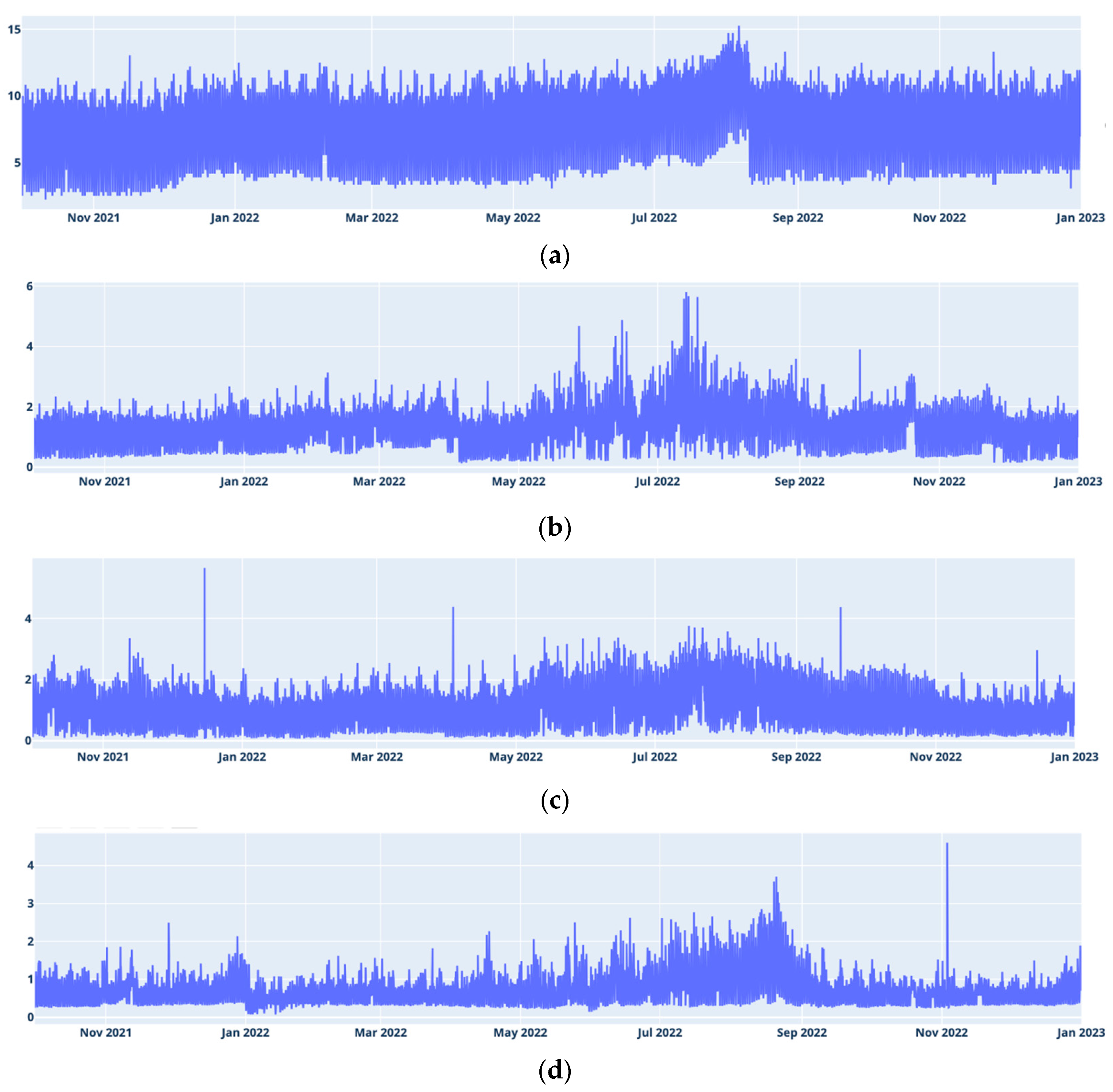
This study uses real water flow measurements from four supply sectors located in rural, low-density populated areas in Portugal: Janeiro de Cima (638 inhabitants), Aldeia de Joanes (1168 inhabitants), Degolados (866 inhabitants), and Alcáçova (4798 inhabitants). Data, which were collected from monitoring systems and stored in databases, were made available by the company responsible for the water supply. Data spanning October 2021 to December 2022 were used for training and testing the predictive models.

Preprocessing involved several steps to ensure data quality and uniformity: concatenating files into a single DataFrame, retaining only the datetime and water flow rate columns and converting data types. Equidistance of the time series data was ensured by interpolating missing values and correcting timestamp anomalies. Data recorded at 5 min intervals were resampled to an hourly frequency by averaging the cleaned and processed data that were exported for the analysis.

3.2. Data Description

The final datasets contained hourly water flow records for each location, structured uniformly for model application. Each dataset provided a comprehensive representation of water flow dynamics, essential for effective time series forecasting.

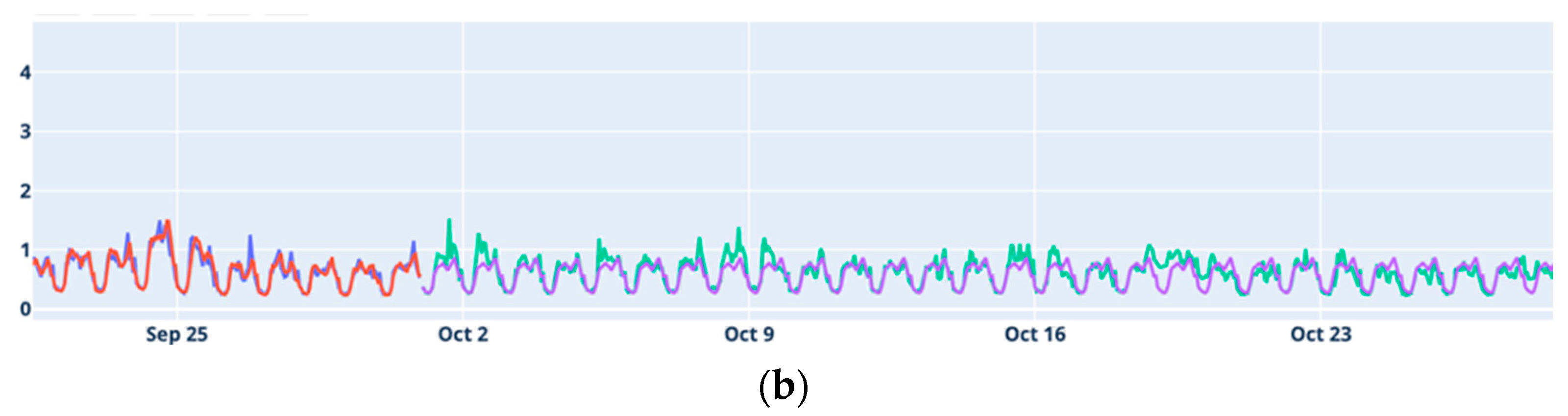
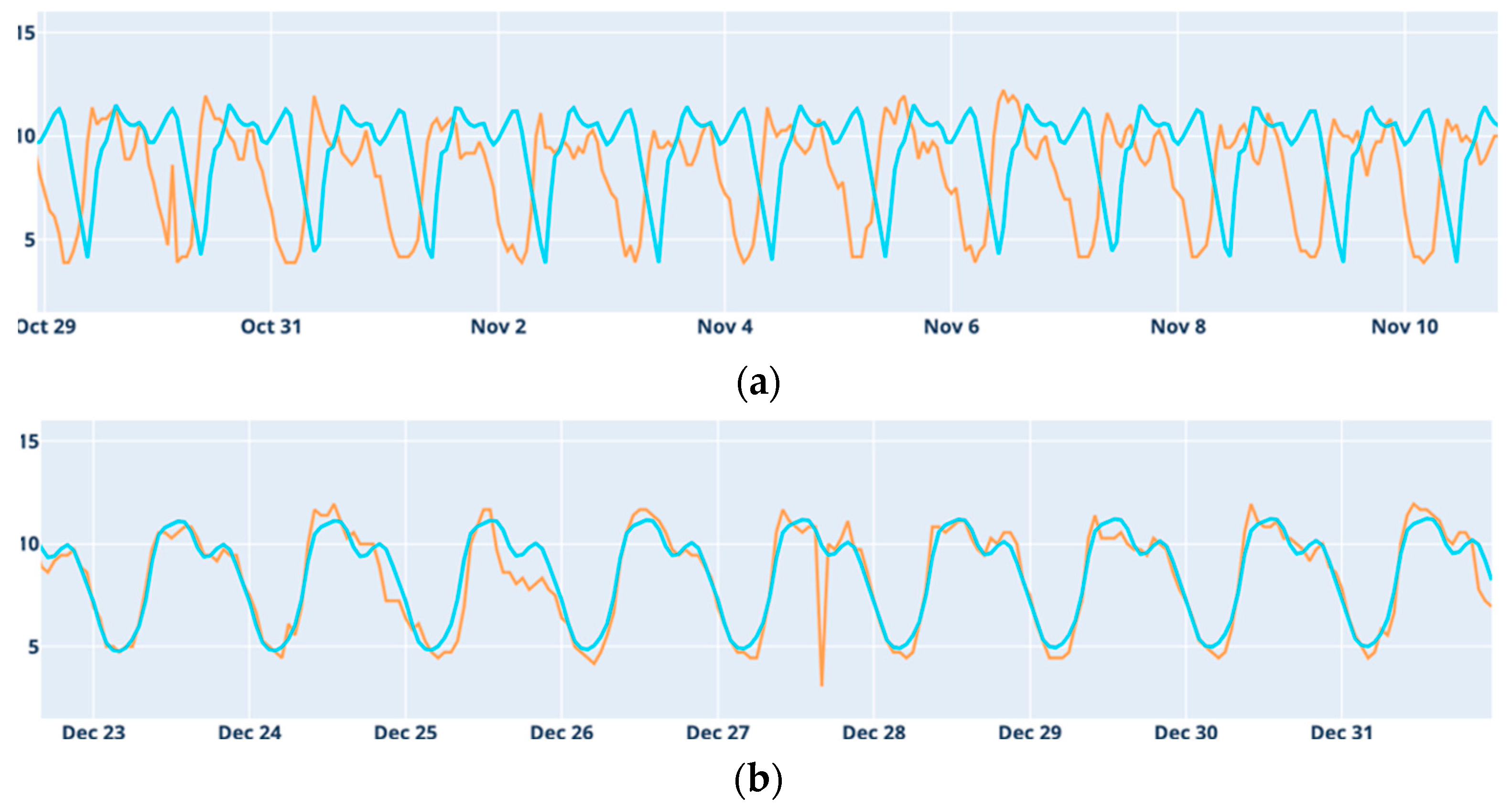
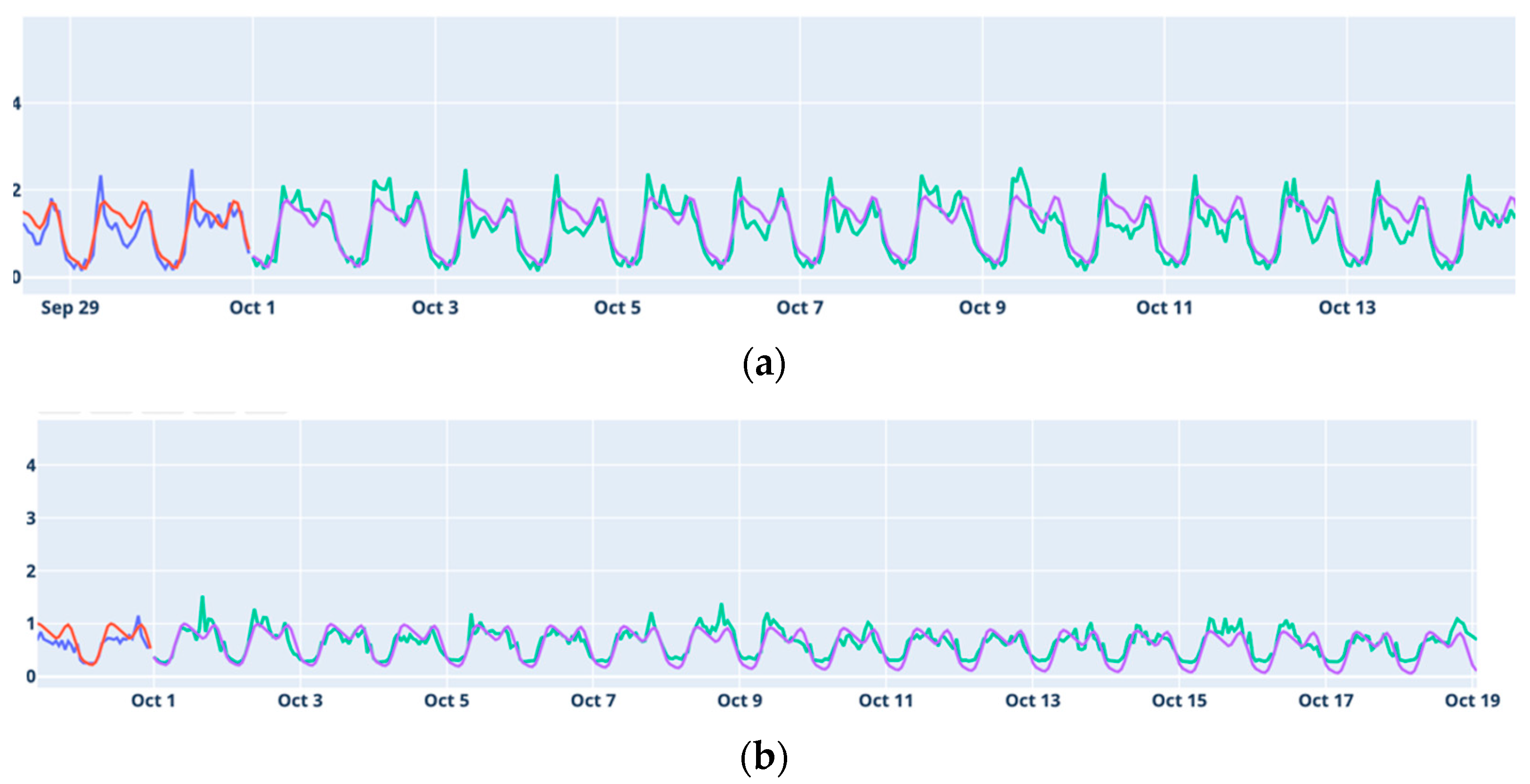
The plots presented in Figure 1 illustrate that each dataset has its own particular characteristics. In Alcáçovas, a significant increase in the average was observed, peaking in August, followed by a sharp decline. This pattern corresponds to a rupture in the distribution network, which was initially undetectable on the surface. Aldeia de Joanes, Janeiro de Cima, and Degolados exhibit high variability, especially during the summer months. These locations are small villages with few permanent residents, but they experience a significant increase in population during the summer, a time when temperatures are also notably high. The effect of the summer is less pronounced in Degolados.

Figure 1. Time series, represented as the plot of the water flow (L/s) over time for the four locations studied: (a) Alcáçova, (b) Aldeia de Joanes, (c) Degolados, and (d) Janeiro de Cima.

3.3. Data Analysis

Data analysis procedures were implemented to prepare and ensure that the time series data meet the assumptions for the forecasting models used. Analyses of the datasets were performed regarding stationarity, autocorrelation, decomposition, and normality distribution assessment. To verify stationarity, the Augmented Dickey–Fuller (ADF) test, the Kwiatkowski–Phillips–Schmidt–Shin (KPSS) test, and the Philips–Perron (PP) test were employed. The ADF and PP tests check for the presence of a unit root, suggesting non-stationarity, while the KPSS test checks for stationarity. Differentiation was applied to transform non-stationary series into stationary ones by computing differences between consecutive observations. The appropriate order of differencing was determined iteratively, followed by re-evaluation using stationarity tests. The autocorrelation function (ACF) and partial autocorrelation function (PACF) plots were used to identify patterns and determine the order of the autoregressive components in the ARIMA model. Time series decomposition was performed to separate the series into trend, seasonality, and residual components using an additive model. To determine if the data followed a normal distribution, the Shapiro–Wilk and Anderson–Darling tests were conducted. These tests assess whether the data deviate significantly from a normal distribution, which is essential for many statistical modeling techniques. In cases where normality was not observed, logarithmic and cubic root transformations were applied to the series, and the normality of the transformed series was reassessed.

For model training and testing, each dataset was divided into a training set consisting of the first 12 months of the time series and a test set including the last 3 months. For the LSTM model, validation data were also necessary: the first 9 months were used for training, the next 3 months for validation, and the final 3 months for testing.

3.4. Parametrization of the Models

This section describes how the four chosen forecasting models were applied to data.

The Holt–Winters method, which applies exponential smoothing to level, trend, and seasonal components, was preferred in its additive form due to the consistent nature of seasonal variations in the data.

The parameters of the ARIMA model were determined using autocorrelation and partial autocorrelation functions and the observed seasonality, aiming to minimize the Akaike Information Criterion (AIC). Residual correlation was also analyzed to finalize parameter selection.

The LSTM models employed in this study included both univariate and multivariate configurations. After optimization, the chosen architectures are represented in Table 1. The input layer is always a matrix of shape (n × 24, k), where n is the number of days considered (n = 10 for medium-term forecasting; n = 30 for long-term forecasting) and k is the number of features considered in each model. The output layer is always a vector of size n × 24 that contains the hourly prediction of the n following days.

Table 1. Architecture for the univariate and the multivariate LSTM networks. n stands for the number of days in the two different time-horizon forecasts considered: 10 days for medium term and 30 days for the long-term forecast.

	Univariate LSTM	Multivariate LSTM
Input layer size	(n × 24.1)	(n × 24.5)
LSTM layer/nb of nodes	1/48	1/24
Dense layer/nb of nodes	1/24	-
Output size	n × 24	n × 24

The univariate model received as input the single time series input, specifically the normalized water flow data. The multivariate model received as input both the normalized water flow time series and four additional variables representing the time information codified by Fourier series decomposition. In both cases, the activation function for the LSTM layers was the rectified linear unit, the optimization algorithm used was the Adam optimizer, and the loss function was the Mean Squared Error.

The parameters for the Prophet model were selected to handle seasonality, trend changes, and holiday effects. The growth parameter was set to “linear”. Yearly and weekly seasonalities were enabled by default, while daily seasonality was added if significant daily patterns were detected. Custom holiday effects were included to account for impactful days, specified based on context and expertise. The seasonality order was adjusted to capture complex seasonal patterns, and the model detected changepoints to reflect significant trend shifts.

3.5. Evaluation Metrics

Model performance was assessed using three key metrics: Mean Absolute Error (MAE), Root Mean Square Error (RMSE), and Coefficient of Determination (R²). MAE (3) provides a direct measure of the average absolute error predictions but is not sensitive to outliers. RMSE (4) captures the standard deviation of prediction errors, emphasizing larger errors due to its quadratic nature. R² (5) indicates the goodness of fit, as it measures the proportion of variance in the observed data explained by the model. In the majority of cases, it is a very reliable indicator for model performance.

The equations of the metrics are as follows:

$$MAE=\frac{{\sum }_{i=1}^N\left|y_i-\widehat{y_i}\right|}{N}$$

(3)

$$RMSE=\sqrt{\frac{{\sum }_{i=1}^N{\left(y_i-\widehat{y_i}\right)}^2}{N}}$$

(4)

$$R^2=1-\frac{{\sum }_{i=1}^N{\left(y_i-\widehat{y_i}\right)}^2}{\sum _{i=1}^N{\left(y_i-\overline{\mathrm{y}}\right)}^2}$$

(5)

where N is the number of observations; $\widehat{y_i}$ is the predicted value for observation $i$; $y_i$ is the measured value of observation $i$; and $\overline{\mathrm{y}}$ is the mean of the observed values.

3.6. Software and Equipment

The computational tasks were performed on a MacBook Pro equipped with a 2.6 GHz Intel Core i7 processor, 16 GB RAM, and AMD Radeon Pro 5300 M GPU Key software that included the Anaconda Navigator for managing Python environments and dependencies; Visual Studio Code as the integrated development environment (IDE) for code development; and Python libraries, including Pandas for data manipulation, statsmodels for statistical modeling, scikit-learn for evaluation metrics, and TensorFlow/Keras [27,28] for the LSTM implementation.

4. Results

This section presents the findings from the pre-treatment and analysis phases, specifically the outcomes of the stationarity and normality tests. It then presents the performance of the various forecasting models applied to the datasets.

4.1. Stationarity and Normality

For the four datasets, the application of numerical tests for stationarity revealed mixed results: the KPSS test indicated that the series were non-stationary, while the ADF and PP tests suggested that the series were stationary. Considering that the KPSS test can exhibit issues with very large samples, which is the case here, and that the other tests indicated stationarity, along with graphical observations, it was concluded that the series exhibited weak stationarity. Additionally, differentiation did not improve the stationarity of the series.

Both the Shapiro–Wilk and Anderson–Darling tests used to assess normality rejected the null hypothesis of normality across the four raw data series, indicating non-normality. Subsequent transformations, such as the logarithmic and cubic root, did not achieve normality for any of the datasets. These results pointed to the necessity of using robust models that do not rely on the assumption of normality for accurate forecasting.

4.2. Performance of Forecasting Models

In this section, the summary of the performance metrics of the models obtained across the four locations is presented. The results presented reflect the best-case scenario for each of the models and locations, according to the descriptions provided.

4.2.1. Holt–Winters Models

Table 2 summarizes the model performance metrics for medium-term (10 days) and long-term (3 months) predictions for the four locations, evaluated both on training and testing datasets, for the Holt–Winters model. The results presented reflect the best-case scenario for each of the models and locations, which were obtained with the logarithmic transformation for Alcáçova, Aldeia de Joanes, and Janeiro de Cima, and the original data for Degolados.

Table 2. Performance metrics of the Holt–Winters model applied to water flow time series from the four locations studied, for the transformations that resulted in best-case scenario: logarithmic transformation for Alcáçova, Aldeia de Joanes, and Janeiro de Cima, and original data for Degolados.

Location	Prediction Type	Training MAE (L/s)	Training RMSE (L/s)	Training R2	Testing MAE (L/s)	Testing RMSE (L/s)	Testing R2
Alcáçova	Medium-term	0.517	0.695	0.915	0.602	0.789	0.867
Alcáçova	Long-term	0.517	0.695	0.915	0.792	1.038	0.802
Aldeia de Joanes	Medium-term	0.184	0.286	0.804	0.305	0.383	0.404
Aldeia de Joanes	Long-term	0.177	0.267	0.828	0.454	0.548	−0.042
Degolados	Medium-term	0.159	0.237	0.868	0.195	0.282	0.791
Degolados	Long-term	0.159	0.237	0.868	0.211	0.289	0.688
Janeiro de Cima	Medium-term	0.109	0.174	0.823	0.102	0.152	0.662
Janeiro de Cima	Long-term	0.109	0.174	0.823	0.118	0.203	0.457

The Holt–Winters model showed varying levels of effectiveness across different locations, generally performing better in Degolados and Alcáçova for both medium-term and long-term predictions, while struggling significantly with long-term predictions in Aldeia de Joanes and Janeiro de Cima. Of special note are the results for Aldeia de Joanes, where the best R² value achieved was only 0.404. This is probably due to the high variability of the dataset, as noted above, which the model was unable to capture.

For illustration purposes, Figure 2 presents the zoom in the transition region between training and testing plots superimposed with the predicted time series for (a) Alcáçova and (b) Janeiro de Cima.

Figure 2. Time series amplified over the transition between training and testing regions superimposed with the Holt–Winters model’s forecast for (a) Alcáçova and (b) Janeiro de Cima.

4.2.2. ARIMA Models

Table 3 summarizes the ARIMA model performance metrics for medium-term (10 days) and long-term (3 months) predictions for the four locations, evaluated both on training and testing datasets. The results presented for each case correspond to the models whose parameterization resulted in the lowest AIC and the least residual correlation.

Table 3. Performance metrics of the ARIMA model applied to water flow time series across the four locations studied.

Location	Prediction Type	Training MAE (L/s)	Training RMSE (L/s)	Training R2	Testing MAE (L/s)	Testing RMSE (L/s)	Testing R2
Alcáçova	Medium-term	0.424	0.569	0.943	0.556	0.724	0.888
Alcáçova	Long-term	0.447	0.594	0.938	0.769	1.009	0.813
Aldeia de Joanes	Medium-term	0.176	0.270	0.825	0.243	0.367	0.451
Aldeia de Joanes	Long-term	0.176	0.270	0.825	0.329	0.452	0.292
Degolados	Medium-term	0.164	0.252	0.850	0.192	0.291	0.779
Degolados	Long-term	0.164	0.252	0.850	0.237	0.245	0.554
Janeiro de Cima	Medium-term	0.141	0.213	0.734	0.094	0.142	0.707
Janeiro de Cima	Long-term	0.141	0.213	0.734	0.137	0.227	0.319

The ARIMA model demonstrated strong performance in Alcáçova for both short- and long-term predictions, with high R² values and relatively low error metrics. Degolados and Janeiro de Cima also showed good results for short-term predictions, but with a noticeable drop in the R² value for long-term predictions. As in the previous model, Aldeia de Joanes, while included in the summary, faced challenges with its predictions due to irregularities in its time series data, affecting the model’s ability to provide accurate forecasts.

Figure 3 presents the time series plots zoomed in the transition region between training and testing superimposed with the ARIMA forecasting for (a) Aldeia de Joanes and (b) Degolados.

Figure 3. Original time series zoomed over the transition between training and testing regions superimposed with the ARIMA model’s forecast for (a) Aldeia de Joanes and (b) Degolados.

4.2.3. LSTM Models

Table 4 and Table 5 summarize the LSTM model performance metrics for medium-term (10 days) and long-term (3 months) predictions for the four locations, evaluated both on training and testing datasets, for the univariate and multivariate model, respectively.

Table 4. Performance metrics of the LSTM model applied to water flow time series from the four locations studied, for the univariate model with standardized training data.

Location	Prediction Type	Training MAE (L/s)	Training RMSE (L/s)	Training R2	Testing MAE (L/s)	Testing RMSE (L/s)	Testing R2
Alcáçova	Medium-term	0.133	0.200	0.890	0.234	0.303	0.759
Alcáçova	Long-term	0.145	0.215	0.875	0.260	0.320	0.730
Aldeia de Joanes	Medium-term	0.137	0.194	0.883	0.334	0.453	0.289
Aldeia de Joanes	Long-term	0.150	0.220	0.870	0.350	0.460	0.250
Degolados	Medium-term	0.124	0.187	0.874	0.234	0.303	0.759
Degolados	Long-term	0.130	0.195	0.865	0.240	0.310	0.745
Janeiro de Cima	Medium-term	0.128	0.190	0.876	0.188	0.252	0.761
Janeiro de Cima	Long-term	0.135	0.200	0.870	0.200	0.260	0.720

Table 5. Performance metrics of the LSTM model applied to water flow time series from the four locations studied, for the approach that resulted in best-case scenario: multivariable model with standardized training data.

Location	Prediction Type	Training MAE (L/s)	Training RMSE (L/s)	Training R2	Testing MAE (L/s)	Testing RMSE (L/s)	Testing R2
Alcáçova	Medium-term	0.416	0.545	0.945	0.780	0.977	0.796
Alcáçova	Long-term	0.416	0.545	0.945	0.744	0.996	0.818
Aldeia de Joanes	Medium-term	0.137	0.194	0.883	0.335	0.442	0.207
Aldeia de Joanes	Long-term	0.137	0.194	0.883	0.334	0.453	0.289
Degolados	Medium-term	0.133	0.200	0.890	0.234	0.303	0.759
Degolados	Long-term	0.133	0.200	0.890	0.188	0.252	0.761
Janeiro de Cima	Medium-term	0.088	0.134	0.818	0.112	0.157	0.639
Janeiro de Cima	Long-term	0.088	0.134	0.818	0.155	0.225	0.329

The multivariate LSTM models generally show an improvement in performance over the univariate models. This is evident in the slightly lower training MAE and RMSE values and slightly higher training R² values for most locations. Testing results also show improvement in multivariate models, though the improvement varies by location. The multivariate models generally have higher R² values during training and testing, indicating better model performance.

Overall, the LSTM model demonstrated strong performance in Alcáçova and Degolados for both medium- and long-term predictions, with high R² values and relatively low error metrics. The model showed worse performance for Aldeia de Joanes, struggling with accuracy, as well as for Janeiro de Cima, particularly in the long-term predictions. The LSTM model was particularly effective in capturing the annual seasonality of the water flow data, which is crucial for accurate long-term forecasting. However, the Aldeia de Joanes dataset presents a high level of variability in the data used as the test period, and its behavior differs significantly from the same period the previous year. Both challenges proved too demanding for the LSTM model to adequately address, leading to limitations in its predictive capabilities for this dataset.

Figure 4 presents the Alcáçova time series plots zoomed in the transition region between training and testing superimposed with the (a) univariate LSTM and (b) multivariate LSTM forecasting models.

Figure 4. Original Alcáçova’s time series zoomed over the transition between training and testing regions superimposed with the LSTM model’s forecast for the Alcáçova (a) univariate model and (b) multivariate model.

4.2.4. Prophet Models

Table 6 presents Prophet model performance metrics for medium- (10 days) and long-term (3 months) predictions for the four locations.

Table 6. Performance metrics of the Prophet model applied to water flow time series from the four locations studied.

Location	Prediction Type	Training MAE (L/s)	Training RMSE (L/s)	Training R2	Testing MAE (L/s)	Testing RMSE (L/s)	Testing R2
Alcáçova	Medium-term	0.643	0.842	0.875	0.700	0.873	0.837
Alcáçova	Long-term	0.643	0.842	0.875	0.717	0.920	0.845
Aldeia de Joanes	Medium-term	0.294	0.401	0.612	0.308	0.379	0.417
Aldeia de Joanes	Long-term	0.294	0.401	0.612	0.421	0.513	0.089
Degolados	Medium-term	0.243	0.327	0.748	0.248	0.306	0.755
Degolados	Long-term	0.243	0.327	0.748	0.226	0.284	0.699
Janeiro de Cima	Medium-term	0.170	0.238	0.667	0.112	0.150	0.671
Janeiro de Cima	Long-term	0.170	0.238	0.667	0.152	0.218	0.373

The Prophet model showed good performance in Alcáçova for both medium- and long-term predictions, with high R² values and relatively low error metrics. Degolados also showed favorable results, especially for medium-term predictions. Janeiro de Cima exhibited moderate performance, with a noticeable drop in the R² value for testing data in the long-term predictions. As in the previous cases, Aldeia de Joanes struggled with both short- and long-term predictions, showing low R² values, as did Janeiro de Cima for the long-term forecasting. The Prophet model was particularly effective in capturing seasonal trends in Alcácova and Degolados. However, the particular characteristics of the test data for the other two datasets proved too demanding for the model, similar to what happened with the previous models.

Figure 5 presents the time series plots zoomed in the transition region between training and testing superimposed with the Prophet model’s forecast for a) Degolados and b) Janeiro de Cima.

Figure 5. Original time series zoomed over the transition between training and testing regions superimposed with the Prophet model’s forecast for (a) Degolados and (b) Janeiro de Cima.

4.2.5. Summary of Performance Models

Table 7 and Table 8 present the metrics of the best-performance models across the four locations, for medium-term and long-term forecasting, respectively.

Table 7. Summary of the best-performing models for medium-term forecasting across the four locations.

Location	Model	Testing MAE (L/s)	Testing RMSE (L/s)	Testing R2
Alcáçova	ARIMA	0.556	0.724	0.888
Aldeia de Joanes	ARIMA	0.243	0.367	0.451
Degolados	Holt–Winters	0.195	0.282	0.791
Janeiro de Cima	ARIMA	0.094	0.142	0.707

Table 8. Summary of the best-performing models for long-term forecasting across the four locations.

Location	Model	Testing MAE (L/s)	Testing RMSE (L/s)	Testing R2
Alcáçova	Prophet	0.717	0.920	0.845
Aldeia de Joanes	ARIMA	0.329	0.452	0.292
Degolados	LSTM	0.188	0.252	0.761
Janeiro de Cima	Holt–Winters	0.118	0.203	0.457

According to the results presented in Table 7, the models that perform better for medium-term forecasting are the statistical models. Among them, the ARIMA model allowed better short-term forecasting in three of the datasets. Despite the issues of autocorrelation evident in these types of time series, as well as the deviation of their distribution from a normal distribution, the ARIMA model presented the best values for the considered metrics in the short term. It should also be noted that the best forecast achieved for Aldeia de Joanes has quite a low R² value, as pointed out previously.

For long-term forecasts, Table 8 does not allow for a robust conclusion about a model that systematically leads to better results. In fact, for two of the datasets, Aldeia de Joanes and Janeiro de Cima, the long-term forecasts obtained present low R² values. To achieve a more conclusive analysis, the average performance metrics of the long-term models across the locations were determined (Table 9). All model results for locations with a Coefficient of Determination lower than 0.50 were disregarded, which meant excluding the results for Aldeia de Joanes and Janeiro de Cima.

Table 9. Average Metrics of Long-Term Forecast Models.

Model	Testing MAE (L/s)	Testing RMSE (L/s)	Testing R2
Holt–Winters	0.211	0.289	0.688
ARIMA	0.237	0.345	0.554
LSTM	0.188	0.252	0.761
Prophet	0.226	0.284	0.699

The results presented in Table 9 show that the best average results were obtained by the LSTM model, with an approximate Mean Absolute Error of 0.19 L/s, a Root Mean Squared Error of 0.25 L/s, and a Coefficient of Determination of 0.76. Therefore, the LSTM model stands out as the model that achieves better results for long-term water flow forecasting, followed by the Prophet model. The LSTM model, compared to the Prophet model, also allows for greater control over tuning its parameters. The Prophet model offers fewer adjustment options, which may limit its flexibility and adaptability to specific data characteristics. Both modern models outperformed the classical models (Holt–Winters and ARIMA) in terms of accuracy and reliability for the long-term forecasting.

5. Discussion

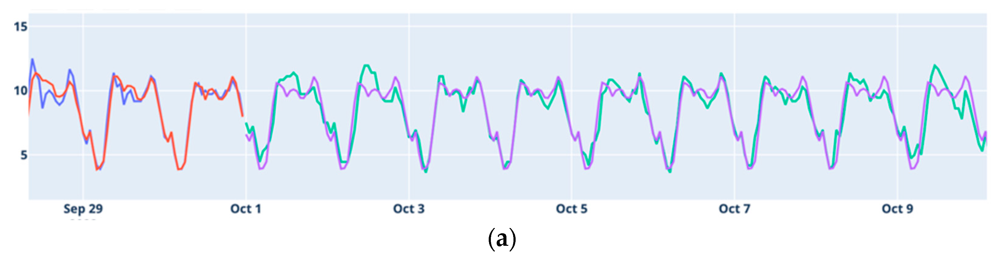
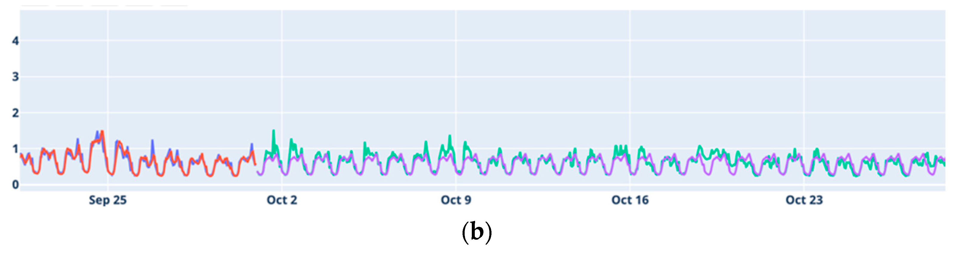
The results obtained in this work show that, overall, the ability to forecast accurately varies significantly by location. Alcáçova and Degolados showed the most reliable forecasting results, benefiting from clear temporal patterns that models could effectively capture. In contrast, Aldeia de Joanes and Janeiro de Cima presented more challenges, particularly for long-term forecasts, likely due to higher data variability and weak seasonal patterns. These findings emphasize the importance of tailoring forecasting models to the specific characteristics of each location’s data to achieve optimal results.

Considering Holt–Winters and ARIMA as classical models and LSTM and Prophet as modern models, the results indicate that the classical models generally perform better for medium-term forecasting. Conversely, the modern models tend to yield better results for long-term predictions.

According to the study referenced in [10], which compares the Holt–Winters model with the ARIMA model, it was expected that ARIMA would significantly outperform the Holt–Winters model. While this was observed to some extent in the medium term, the difference was not substantial. Surprisingly, in the long term, the Holt–Winters model performed better than ARIMA. This underperformance of the ARIMA model can be attributed to certain characteristics of the data series, such as poor stationarity, high autocorrelation, and a distribution far from normal. These factors likely impacted its effectiveness.

Contrary to the findings in [15], which suggest that neural network-based models perform well only for short-term horizons (predicting the next value), our results show that the LSTM model tested in this study provided better long-term forecasts. This model was evaluated in a manner that mimicked its application in a production environment, predicting value by value and compiling the results. When comparing our findings with the existing literature, where LSTM models often show extraordinary results under controlled laboratory conditions (e.g., [29]), we concluded that our results are more realistic and reflective of actual performance.

Regarding the ability to capture seasonality, all four models adjusted well to daily seasonality. However, only the LSTM and Prophet models managed to capture annual seasonality effectively. The Holt–Winters and ARIMA models did not account for patterns from the same period in the previous year, being more influenced by recent data leading up to the forecast period. This implies that these models lose accuracy when series exhibit strong seasonal patterns. This limitation of the ARIMA model was also noted in [22] during a comparison with the Prophet model.

On the other hand, the LSTM and Prophet models showed strong tendencies to adhere to annual seasonal patterns. This contradicts the implications in [22], which suggested that the LSTM model might not handle annual seasonality well. The Prophet model demonstrated a good fit for both daily and annual seasonality. However, it exhibited a significant limitation in the amplitude of its forecast curves. This limitation was particularly noticeable for series with high variability in maximum flow values during summer (Aldeia de Joanes and Janeiro de Cima). This raises concerns about the Prophet model’s accuracy if the forecast period includes the summer, as it might significantly under-predict the actual values. This is of special concern in datasets corresponding to low-population-density areas where the population increases significantly during summer, such as in the cases of Aldeia de Joanes and Janeiro de Cima.

The LSTM model proved to be the best at respecting annual seasonality, making predictions based on what happened in the same periods of the previous year. It only encountered issues during the transition period between training and testing, making it difficult to achieve good medium-term forecasts.

The Prophet model showed performance comparable to the LSTM model regarding annual seasonality. However, its limitation in the amplitude of predictions prevented it from achieving better results.

For the ARIMA and Holt–Winters models, the inability to implement annual seasonality renders them accurate for medium-term forecasting but imprecise for long-term forecasting. In a water distribution network, if the number of breaks continues to increase, these models will be unable to alert us as they do not consider the need to make predictions based on similar periods in previous years.

This work has some limitations. A primary constraint was the quality and availability of historical data, as incomplete, noisy, and high-variability data can lead to inaccuracies. Most notably, for one of the datasets used in this work (Aldeia de Joanes), none of the models provided satisfactory results for either medium-term or long-term forecasts. Similarly, for another dataset (Janeiro de Cima), none of the models used for long-term forecasting provided satisfactory results. Each forecasting model, including ARIMA and Holt–Winters, has inherent limitations; for example, ARIMA struggles with non-stationary data and pronounced seasonal patterns, particularly for long-term predictions. The complexity of selecting optimal parameters and the significant computational resources required for training advanced models like LSTM further constrained this study. Additionally, the findings and models are tailored to the specific dataset used, raising concerns about their generalizability to other datasets without further adjustments. The effectiveness of multivariate models is also heavily dependent on the careful selection and preprocessing of input features, where suboptimal choices can degrade model performance. Furthermore, this study does not incorporate additional external variables (e.g., climatic factors) that could potentially enhance forecasting accuracy, especially for modern models like LSTM. These limitations underscore the challenges in developing accurate and robust forecasting models, highlighting the need for meticulous data handling, model tuning, and validation. Further research could focus on the investigation of hybrid models for improvement in a water demand forecast. Hybrid models combining classical and deep learning approaches have been studied for water demand forecasting problems. For instance, combining ARIMA with a type of neural network called the General Regression Neural Network improved daily water forecasting in Saudi Arabia [30]. Another study found that a hybrid model with Holt–Winters, ANN, and SARIMA performed best for industrial water consumption forecasting [25]. More recently, advanced hybrid methods using different machine learning approaches, such as Convolutional Neural Networks, LSTM, and LSTM with attention mechanisms, have been exploited for water demand forecasting and have been shown to lead to very promising results [23].

6. Conclusions

In conclusion, this study underscores the significant importance of selecting appropriate time series forecasting models for efficient water management in distributed supply networks. By comparing classical models such as Holt–Winters and ARIMA with modern approaches like LSTM and Prophet, we demonstrated that the choice of model greatly impacts the accuracy and reliability of both medium-term and long-term forecasts. The results reveal that while classical models perform well for medium-term predictions, modern models, particularly LSTM, excel in long-term forecasting due to their ability to capture complex seasonal patterns. This insight is vital for water distribution networks, which require precise and reliable predictions to optimize resource allocation and minimize operational costs. Future research should focus on integrating additional external variables and exploring hybrid models to further enhance forecasting accuracy.