Article

Constructing a Machine Learning Model for Rapid Urban Flooding Forecast in Sloping Cities along the Yangtze River: A Case Study in Jiujiang

1
Key Laboratory of Mine Spatio-Temporal Information and Ecological Restoration, Henan Polytechnic University, Jiaozuo 454000, China
2
Shanghai Investigation, Design & Research Institute Co., Ltd., Shanghai 200335, China
3
Kunming Surveying and Mapping Institute (Kunming Management Office of Urban Underground Space Planning), Kunming 650051, China
4
Three Gorges Smart Water Technology Co., Ltd., Shanghai 200335, China
*
Author to whom correspondence should be addressed.
Water 2024, 16(12), 1694; https://doi.org/10.3390/w16121694
Submission received: 20 March 2024 / Revised: 24 May 2024 / Accepted: 12 June 2024 / Published: 14 June 2024
(This article belongs to the Section Urban Water Management)

Abstract

:
Cities with sloping terrain are more susceptible to flooding during heavy rains. Traditional hydraulic models struggle to meet computational demands when addressing such emergencies. This study presented an integration of the one-dimensional Storm Water Management Model (SWMM) and the two-dimensional LISFLOOD-FP model, where the head difference at coupled manholes between the two models functioned as the connection. Based on its calculation results, this study extracted the characteristic parameters of the rainfall data, simplified the SVR calculation method and developed a high-efficiency solution for determining the maximum ponding depth. The cost time of this model was stable at approximately 1.0 min, 95% faster compared to the one from the mechanism model for 5 h simulation under the same working conditions. By conducting this case study in Jiujiang, China, the feasibility of this algorithm was well demonstrated.

1. Introduction

In recent years, big data methods have gradually been applied to urban flooding, stormwater management, and other related fields [1,2,3,4]. The integration of multi-source information, such as satellite radar and precipitation data, along with extensive data mining and intelligent analytical methods, has become the focal point of high-precision information identification in the hydrological field. Scholars have conducted extensive research on flood forecasting and numerical simulation of urban flooding. For example, Pedrozo-Acuna et al. [5], Mignot et al. [6], and Audrey Douinot et al. [7] have successively used various simplified methods to simulate the flood process. Payande et al. [8] and Papaioannou et al. [9] utilized the MIKE21 FM model to assess the risk of flooding under various operational conditions. Chang et al. [10] and Huang et al. [11] conducted a flooding simulation analysis using GIS and SWMM models. Ma et al. [12], Guo et al. [13], Wei et al. [14], and Wang et al. [15] utilized the MIKE21 FM model to simulate the inundation evolution process of Beijing City, Liaojiang flood storage area, Mengwa flood storage and detention area, and Ningjinbo and Daluze flood storage and detention areas. The research above has conducted further explorations in multi-source information fusion, information mining, and intelligent algorithms and has achieved specific functionalities. However, the hydrological features of steep slopes and rapid water accumulation in sloping cities result in extremely fast urban flooding, and current traditional hydraulic models cannot meet this challenge.
In contrast to the traditional hydraulic model, the flooding forecast model constructed on rainfall in time series has showed its merits by simplifying the model and reducing the data demand. Zheng et al. [16] constructed a bivariate STARMA model to fit the precipitation and water accumulation sequence process and perform short-term prediction of water accumulation. Li et al. [17] coupled the data assimilation method of support vector machine SVM and Ensemble Kalman Filter (EnKF) for real-time flood forecasting. Rjeily et al. [18] used a nonlinear autoregressive (NARX) neural network with external inputs to develop a flood forecasting system for effective management and flood prevention and mitigation. The data-driven model proposed in the previous studies did increase the flood calculation speed responding to precipitation, yet the mechanism relating precipitation and flooding was ignored, which made the result less reliable. Yan et al. [19] established a SVM model to expedite the prediction of maximum flood depth within the region, with a high accuracy based on feeding the hydraulic model results as training set. However, the detailed description of ponding map was of the same importance of the max depth for implementing advanced controls.
This study was a case study in Jiuajing, China aimed to yield some insights on the feasibility of enhancing the calculation efficiency and reliability by proposing a one-dimensional (1D) and two-dimensional (2D) coupling algorithm and applying the mechanistic results to a machine learning model. Simultaneously, attempts were undertaken to forecast the maximum flood depth across all grids within the area and to craft a comprehensive maximum flood depth map.

2. Research Methods

2.1. Study Area

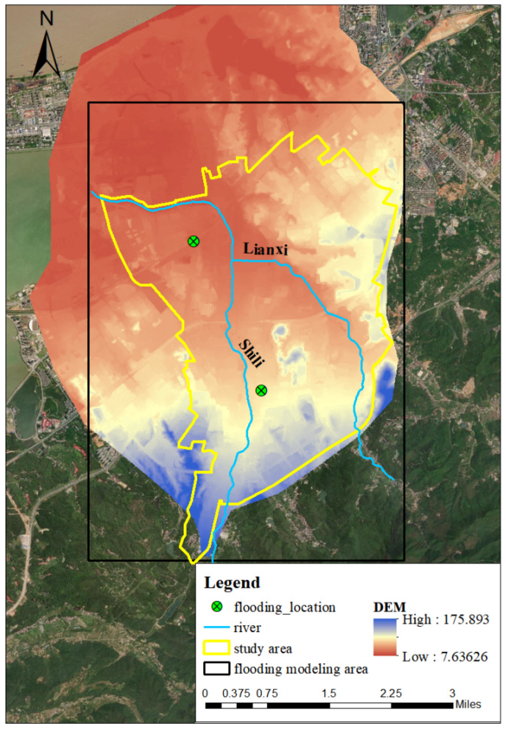
The study area is located in Jiujiang, China. The urban area of Lianghe is higher in the southwest and gradually decreases towards the north. There are two main rivers running through, called Shili River and Lianxi River (Figure 1). The downstream Bali Lake covers approximately 18 km2 and is separated from Yangtze River by gate. The water level of Bali Lake is regulated to remain at around 16.12 m during the dry season and 16.62 m during the rainy season.
The drainage system within the modeling area consists of both a combined system and a separate system, with a total pipe network length of approximately 250 km. There is 1 wastewater treatment plant (WWTP) in the modelling area and 1 WWTP located at the downstream outsides, referred to as WWTP1 and WWTP2. Rainfall data are collected from 5 gauges located in Jiujiang, with 2 stations situated within the modeling area.
The flooding occurs at the main roads beneath the railway in Lianghe (Figure 2), where is relatively lower compared to the surrounding. This topography characteristic makes the area suffer a high risk of flooding during even moderate rainfall events yet there is no satisfactory solution for mitigation.

2.2. Methodology

The flow chart of methodology applied in this study was presented in Figure 3. It could be divided into 3 parts: the construction of a coupled model engine of 1D drainage system model and 2D overland flow model; the construction of detailed coupled model of study area; the integration of coupled model and machine learning model.

2.2.1. 1D Drainage System Model and 2D Overland Flow Model

Both 1D and 2D models were introduced in this study, namely the stormwater management model (SWMM) and LISFLOOD-FP, respectively.
The Storm Water Management Model (SWMM) was developed by the U.S. Environmental Protection Agency (EPA) to address stormwater runoff in urban areas. It can dynamically simulate the runoff from slopes caused by a single precipitation event or continuous rainfall. This simulation tool is widely utilized in the design, planning, and operation of stormwater runoff, combined sewerage system, sewage pipe systems, and urban water systems in urban areas. The hydraulic module in SWMM software 5.1 can conduct hydraulic simulations of facilities such as pipelines, channels, water storage and treatment units, and water distribution buildings.
LISFLOOD-FP is a grid-based hydraulic model that has been applied in various fields of earth science, such as terrain dynamics modeling, urban drainage modeling, population flow modeling, coastal flood modeling, uncertainty quantification, and coupled hydraulic modeling. Since its inception, it has undergone numerous developments and tests, gradually evolving into the latest tool for flood modeling applications at various scales, including catchments, cities, and river basins. LISFLOOD-FP offers a range of built-in numerical calculation schemes for solving 2D shallow water equations of varying complexity. These include simple diffusion wave calculations as well as more advanced finite volume and Galerkin finite element schemes capable of solving complete shallow water equations.

2.2.2. Coupling of 1D and 2D Models

The integrating 1D and 2D model addressed the water exchange process between urban underground drainage system and overland runoff. The vertical interaction occurs at specific structures, such as manholes and storage units, which were collectively referred to as junctions, in the rest of the paper.
The water level at these junctions was denoted as Depth1d, while the water level at the corresponding surface grid was referred as Depth2d.The interaction between these two systems can be categorized into three distinct situations [20] (Figure 4):
Depth1d > Depth2d, while the junction water level was higher than the surface water level at the corresponding position. At present, the water flow in the pipe network system was outflowing through the junctions into the surface flow, and the water flow was transitioning from the 1D model to the 2D model.
Depth1d < Depth2d, while the water level at the junctions was lower than the surface water level at the corresponding position. The water flowed from the surface to the underground drainage pipe network, and the water flow entered the 1Dmodel from the 2D.
Depth1d = Depth2d, while the surface water level was equal to the junction water level, or there was no water on the surface and the junction water level was lower than the surface elevation, the surface and groundwater flow did not exchange.
Due to the lack of in-depth research on the mechanism and calculation methods of vertically connected water flow exchange, the fundamental theory of vertical flow exchange was still in its early stages of development, and the available calculation methods were limited. In this study, the weir and orifice flow formulas were used to calculate the exchanged water volume at the vertical interaction.
(1)
Junction outflow
The orifice flow formula was used to calculate the junction outflow, taking into account the water flow status of the pipe network.
1. Utilized the orifice flow formula to calculate the volume of water outflowing. If outflow occurred at the junction, the exchanged water volume was calculated using the following formula based on the junction water level (Depth1d); the surface grid water level (Depth2d) was calculated by the two-dimensional model at the corresponding position of the junction and the orifice area. By applying the following formula, the volume of water exchanged during the outflow event can be determined.
Q n s = c o A 2 g ( D e p t h 1 d D e p t h 2 d )
where c 0 is the orifice flow coefficient with a value range of 0~1; A represents the orifice area, m2; g is the gravity acceleration, 3/s; D e p t h 1 d and D e p t h 2 d are the water levels of the junction and the surface at the current time step, respectively, m; Q n s is the calculated outflow amount of the present time step, m3/s.
2. Calculated the total inflow of the junction using the results from SWMM and ensured that its outflow in the next time step did not exceed the total inflow of the junction ( Q t o t a l i n f l o w ). At the same time, the maximum allowable junction outflow can also be set according to the actual situation Q o u t m a x . As a result, the junction outflow was ultimately limited by the following formula to ensure model stability.
Q n s = m i n ( Q t o t a l i n f l o w , Q o u t m a x , Q n s )
3. Used the outflow volume as the external outflow of the SWMM model junction and as the source term for the two-dimensional grid in LISFLOOD-FP for the subsequent time step calculation.
(2)
Surcharged flow
The surcharged flow was calculated by combining the weir flow and orifice formulas. The steps are as follows:
1. Calculated the surcharged flow. The nodal water levels and the corresponding grid water levels D e p t h 2 d were obtained by the simulation results of SWMM and D e p t h 1 d resulted from the two-dimensional simulation model. According to the difference in water levels, the surcharge flow was calculated using the following formula:
Q s n = c w · w · d e p t h 2 d 2 g · d e p t h 2 d    D e p t h 1 d Z < D e p t h 2 d c o A 2 g D e p t h 1 d D e p t h 2 d    Z < D e p t h 1 d D e p t h 2 d
where c w is the weir flow coefficient with the value range of 0~1; w is the junction perimeter or rainwater outlet width, m; Z is the maximum value of the 1D ground elevation and the 2D ground elevation, m a x ( Z 1 d , Z 2 d ) , m; d e p t h 2 d is the surface water depth, D e p t h 2 d Z , m; Q s n is the junction return flow, m3/s.
2. To ensure the stability of the model, the following formula was used to restrict the surcharged flow:
Q s n = m i n ( Q s n , Q i n m a x , V / t n + 1 )
where Q i n m a x is the maximum allowable return flow, which is given according to the actual situation, m3/s; V is the two-dimensional grid water volume at the connection with the junction, m3; t n + 1   is the next time step.
3. The surcharged flow was incorporated into the SWMM model as the external inflow of the junction. In the two-dimensional model LISFLOOD-FP, the surcharged flow was designated as the source term and updated to the next time step.

2.2.3. SVR

In the field of hydrological forecasting, the Support Vector Machine (SVM) has been widely used, such as for rainfall and runoff forecasting, flooding forecasting, streamflow and sediment yield forecasting, etc. [18]. SVM offers distinct advantages in addressing challenges such as small sample sizes, nonlinearity, and high-dimensional pattern recognition. It extends its usefulness to various machine learning problems, including function fitting. SVM operates based on the principles of the VC dimension theory from statistical learning and the minimum structural risk principle. Drawing from a limited sample, the SVM aims to find a balance between model complexity (which reflects learning accuracy for a specific training sample) and learning capability (the ability to identify samples without errors). This balancing act is crucial for achieving optimal generalization capability.
Support vector regression (SVR) is a significant application branch of the SVM, designed specifically to tackle regression problems. It optimizes the model by minimizing the overall loss and narrowing the width of the interval band. The underlying principle of the SVR nonlinear model involves converting input space samples (“x”_i, “y”_i), where i = 1, 2, …, n, through a nonlinear mapping “ϕ.” This process involves transforming the samples into a high-dimensional feature space and then using a linear regression method to solve the regression function within the feature space.
y = ω × ϕ x + b
In the formula, xi is the input quantity; yi is the output quantity; ω is the weight vector; b is the offset amount. To ensure that the predicted y value closely aligns with the actual value, with the error between y values not exceeding the insensitivity coefficient ε, the optimization problem was formulated as follows:
m i n 1 2 w 2 s . t . { y i ω × ϕ x i b ε ω × ϕ x i + b y i ε   ( i = 1,2 , · · · , l )
The corresponding regression function is expressed as:
f x = i = 1 l α i α i * K x i , x + b
In regression prediction, the kernel function has a significant impact on the accuracy of predictions. Commonly used kernel functions include the Gaussian radial basis, linear function, and polynomial function. Given that collected data is susceptible to noise interference, it is challenging to balance prediction accuracy and noise robustness. Therefore, a combined kernel method that incorporates both the polynomial and RBF kernels is employed. The expression for the integrated kernel function is:
K x , x 2 = p × e x p   x x 2 2 × 0.1 2 + 1 p × ( x × x 3 + 1 ) 3

2.2.4. Integrating Model of Mechanism and Machine Learning Models

The mechanism model evaluated the hydraulic performance of drainage system corresponding to different rainfall data. The simulation speed of this coupled flood model was dominated by the detailed 1D SWMM model, whose simulating time step had to be short to be precise. Moreover, while encountering heavy rain in a short period, the impact of rivers and lakes on the urban drainage system could be eliminated. Therefore, the flood risk under the influence of the drainage system could be independently assessed.
In this integrating model of the mechanism and ML model, parameters such as rainfall, processes including runoff, overflow, and consequence of ponding were evaluated presented mechanism model. Its outcome of max ponding depth represented the principles of interaction within the whole system, which would be learned by the SVR model, to capture the nonlinear relationship between input and output, from rainfall to max ponding depth.

3. Model Construction

3.1. Coupling Model Construction

3.1.1. 1D Drainage System and River Model

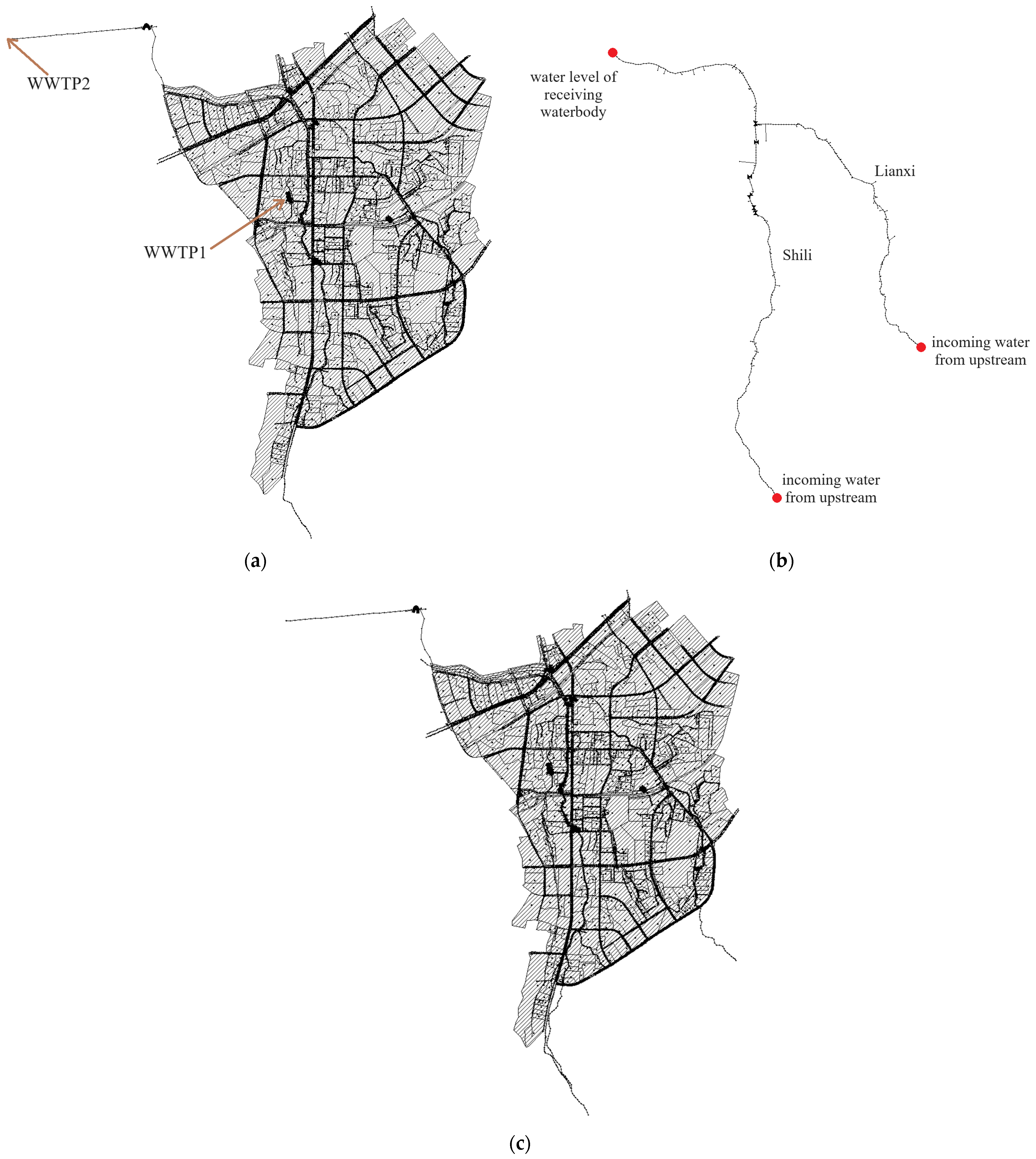
A SWMM model was established for the integrated system including drainage system and rivers. The sketched network system was illustrated with 8040 manholes, 8090 pipes, 151 outlets and 357 sub-catchments in the final model (Figure 5a).
The Horton model was employed to calculate infiltration. Considering the soil in the study area was predominantly clay, it was determined that the maximum and minimum infiltration rates were 51 mm/h and 3 mm/h, respectively, and the infiltration attenuation coefficient was 4. The maximum detention volumes in the permeable and impermeable areas were initially selected to be 2 mm and 0.14 mm, respectively.
The land use contributions for each subcatchment were evaluated using Landsat 8 remote sensing images. The Manning coefficient for the permeable surface and the non-permeable surface were estimated to be 0.2 and 0.012 based on the recommendation.
The Manning coefficient of concrete pipes was initially selected as 0.013 while the head loss coefficients for pipe inflow and outflow were set to 0.15 and 0.015, respectively.
The dry weather flow (DWF) and pattern of each residence unit within the study area were collected and analyzed from the community or from the monitor data.
The Shili River (8.8 km) and Lianxi River (5.2 km) within the study area are illustrated in Figure 5b. The model incorporates a total of 351 cross sections with a roughness coefficient set at 0.055. The downstream water level was set to be 16.12 m since hydraulic performance in the receiving Bali Lake was stable. It was assumed that upstream-moving water was 0.5 m3/s for both rivers.
The network model and river model were integrated by coupling outlets to the corresponding river sections, describing the water exchange within two systems based on their hydraulics performance (Figure 5c).
The precipitation boundary for the integrated 1D model was varying in spatial, calculated according to the contributions of 5 rain stations using inverse-distance-weighted (IDW), with a time resolution of 5 min.

3.1.2. Coupling of 1D and 2D Model

The Digital Elevation Model (DEM) data in LISFLOOD-FP was obtained by oblique photography, with an accuracy of 1 m × 1 m. Special terrains, such as those under bridges and dams, were processed separately to ensure an accurate result of ponding for places with comparatively lower elevation.
The DEM data was interpolated into an ASCII format as required by LISFLOOD-FP, resulting in a 5 m grid with 1220 columns and 1782 rows, 2,174,040 grid cells in total, as illustrated in Figure 2. It was assumed that all the manholes and outlets (referred as junction in SWMM model) except pressured manholes were supposed to be coupled with the overland model. The final amount of coupled junction was estimated to be 8173.

3.1.3. Calibration and Verification

The SWMM model played a dominant role in the presented coupling model, as it primarily estimated the exchange process between the drainage system and the surface based on the conveyance capacity of pipes and manholes. Therefore, the calibration and verification of the integrated model would be conducted subsequently, while the SWMM model was calibrated and verified first to ensure accurate hydraulic results.
The key parameters in SWMM model requiring adjustment included the infiltration rate in the Horton’s model, the impervious rate, and the width of each subcatchment. These adjustments would have a significant impact on both the runoff concentration time and the flow peak. The parameter requiring refinement in the coupled model was surface roughness, which directly affected the flow movement between the grids.
In this study, The Nash–Sutcliffe efficiency coefficient (NSE) was employed for both coupled model calibration and verification. The NSE is the most widely used objective function in the model calibration process and is also an important numerical index for evaluating simulation effects [18], especially for data in time series. According to the calculation formula, the difference between the observed rate and the simulated rate is in the form of a square, which will give the peak section a higher calculation weight. The NSE is therefore more sensitive to the peak difference [21].

3.2. ML Flooding Model Construction

3.2.1. Data Collection and Processing

The raw data for training and validating SVR model consisted of ponding depth and precipitation, both of which varied in space and time. The treatment of raw precipitation data was addressed in Section 3.1. The flood map could be obtained by interpolating ponding depths and ground elevation from enough ponding depth monitors, or by performing the coupled flood model with a high accuracy reliability.
As mentioned in Section 3.1.2, there were nearly 2 million grids in the DEM ASCII file used for overland runoff simulation. Most of these grids represented land values or areas with a minor risk of flooding, such as green spaces or elevated residential and industrial zones. To train the model effectively, it was essential to select target grids based on simulation outcomes. The selection criterion was established as grids that experienced flooding in at least one scenario.

3.2.2. Feature Engineering

The input features were determined based on the acknowledge on urban flooding mechanism, generally including rainfall and water levels at outlets. In this study, water level at outlet was exclusive, as the downstream water level of the Shili River was assumed to be stably controlled by the receiving lake, while the water levels at the outlets along the river were parameters interacted with inside the 1D coupling. To reduce the dimensions of input, the rainfall data in time series were characterized as maximum intensity (mm/5 min), accumulated volume (mm), and duration (h).

3.2.3. Hyperparameters Selection

The SVR model uses the radial basis function (RBF) as the kernel function. The penalty factor for the error term, denoted as C, is set to 1000 to improve the model’s accuracy in handling light rainfall. The default values for the coefficient of the kernel function (gamma) and the training convergence coefficient (epsilon) are retained.

3.2.4. Training and Validating

A hybrid set of designed and observed rainfall events was divided into the training set and the validating set based on the ratio of 70% and 30%, and the other measured rainfall events were used as the test set.

3.2.5. Model Evaluation

The coefficient of determination (R2) was a widespread applied choice for the calibration numerical index of the ML model. Considering the SVR model output maximum depth rather than a time-varying series of depths, the absolute error was a more suitable numerical index for model evaluation.

4. Data

4.1. Monitor Data for Model Calibration and Validation

From June to August 2023, monitors were deployed in Lianghe, including five flow monitors (q) and one ponding depth monitor (d). Throughout installation, four rainfall events were observed, providing data for model calibration and verification. Table 1 presents a summary of the four rainfall events and the corresponding available monitors. These four events comprised dry time and rainy time, which were divided into single rainfall events according to the criteria as follows:
(1)
The rainfall was considered to end if there was no rain for the following 6 h.
(2)
The accumulated rainfall volume of a single rainfall event was assumed to be more than 1 mm.
(3)
Since there were multiple rain gauges in function, the analysis was conducted individually for each gauge, and the amalgamation of periods was the eventual outcome for single rainfall event division.

4.2. Simulation Data for SVR Model Training

As mentioned above, only one ponding depth monitor was available in the whole study area. To achieve a comprehensive depiction of the flooding map within the entire area, multiple simulations under various design rainfall using the verified coupled model were carried out to generate ponding depth as training data for the SVR model.
The design rainfall was computed utilizing the rainstorm intensity formula of Jiujiang (Formula (9)).
q = 2307 ( 1 + 0.6 l g P ) ( t + 8 ) 0.7
where q is the rainstorm intensity [L/(s·hm2)]; P is the rainfall recurrence interval (year); t is the design rainfall duration (min), where t = t1 + m × t2; t1 is the groundwater collection time (min), depending on the distance, terrain slope and ground coverage, ranging from 5 to 15 min; m is the reduction coefficient, with m for concealed pipes ranging from 1 to 1.5, and m for open channels takes a value of 1.2; t2 is the rainwater flow time in the canal (min).
The Chicago rainfall pattern, with a rain peak coefficient of 0.4, was employed to deduce the rainfall in time series. Table 2 presents all the designed scenarios used in this study. The 27 designed events and 4 observed events (1#1, 2#1, 2#2, 2#3) were divided into the training set and the verification set, while event #3 and #4 were the test set as discussed in Section 2.2.4.
Monitoring data collected from events 3# and 4# were utilized for validating the SVR model, and two primary flooding locations (Figure 2) were specifically chosen to validate the accuracy of the trained SVR mode.

5. Results and Discussion

5.1. Calibration and Validation Results of the Coupled Model

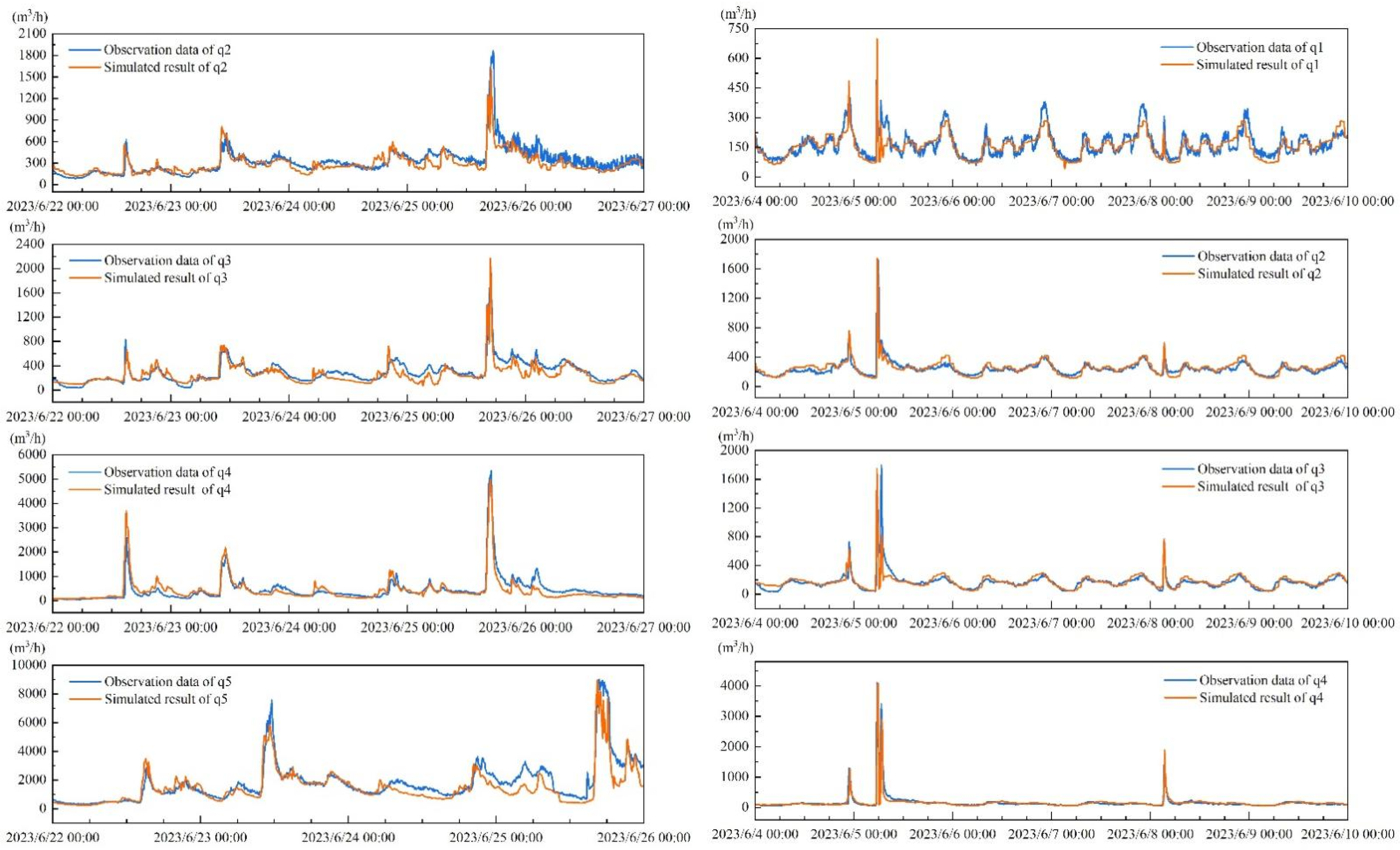
By modifying the parameters as mentioned above, the calibration and validation results of 1D hydraulic model at specific locations were shown in Figure 6, with average NSE as 0.74 and 0.69, respectively. The simulation of calibrating and validating lasted for several days, consisting of dry weather and rainfall. The high level of consistency observed between the simulated and monitored data demonstrated its effectiveness of capturing the hydraulic performance of the drainage system continuously. Hence, this presented 1D model met the accuracy requirement for coupling.
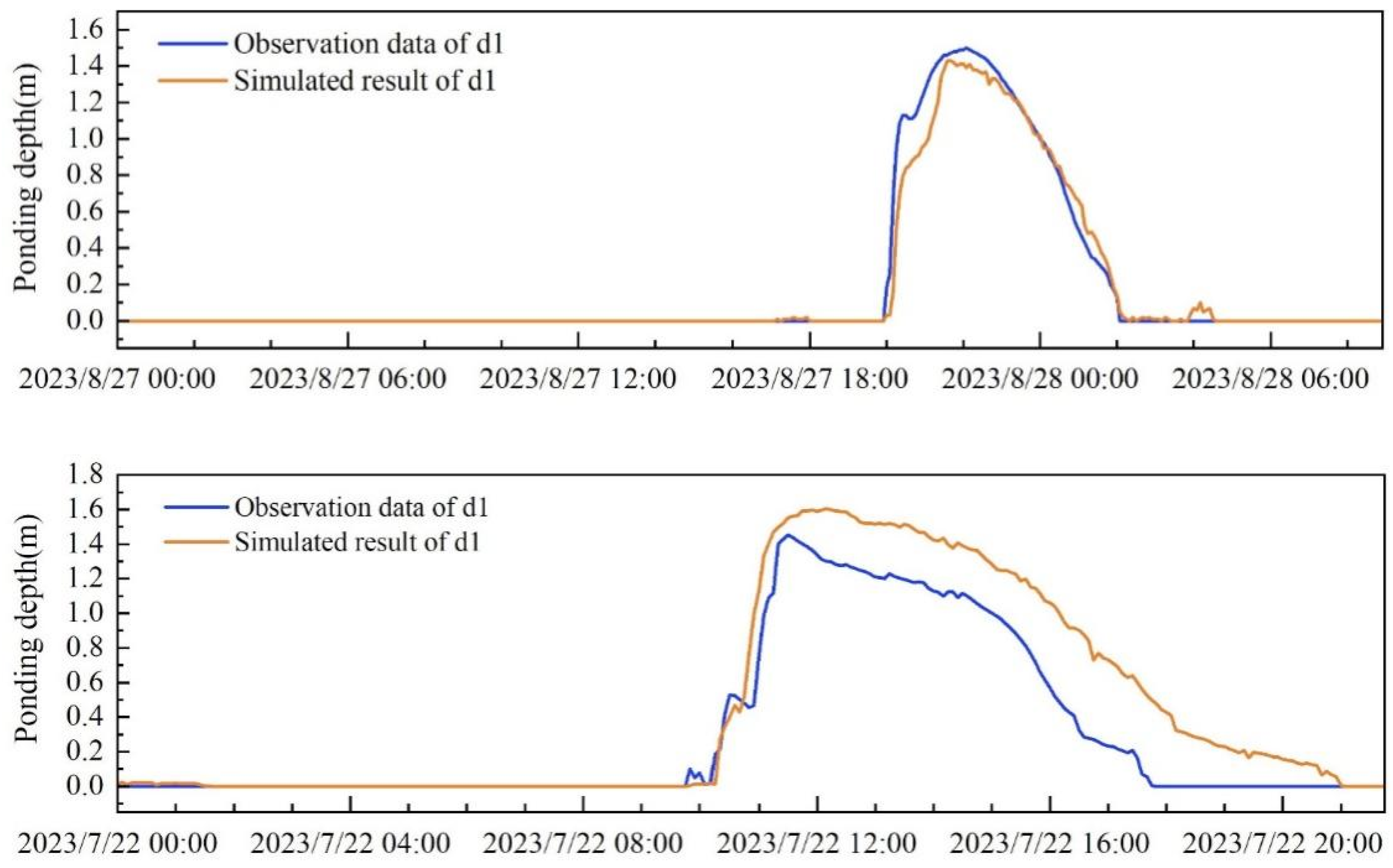
The calibration and validation results of the 2D flood model at location d1 are shown in Figure 7. The calibrated NSE was evaluated to be 0.96, closely aligned with the measured result. For validation result, the absolute error of maximum ponding depth was approximately 12%, and the line indicating simulated ponding mitigation process was below the observed one, yet the appearance time of ponding and the speed of ponding decrease were well described.
It was necessary to address that while calibration and validation, the precipitation data was assumed to be a precise input to the model. The interpolation method for spatial precipitation was meant to compensate the deviation to some extent comparing to barely applying isolated rain gauge data. To increase the reliability of precipitation could be achieved through high-density implementation of rain gauge stations.
Despite the inevitable difference in rainfall, this coupled model was believed to fulfil the accuracy requirement to support subsequent analysis. It was therefore employed to provide training data for the SVR flood model.

5.2. Calibration and Validation Results of SVR Model

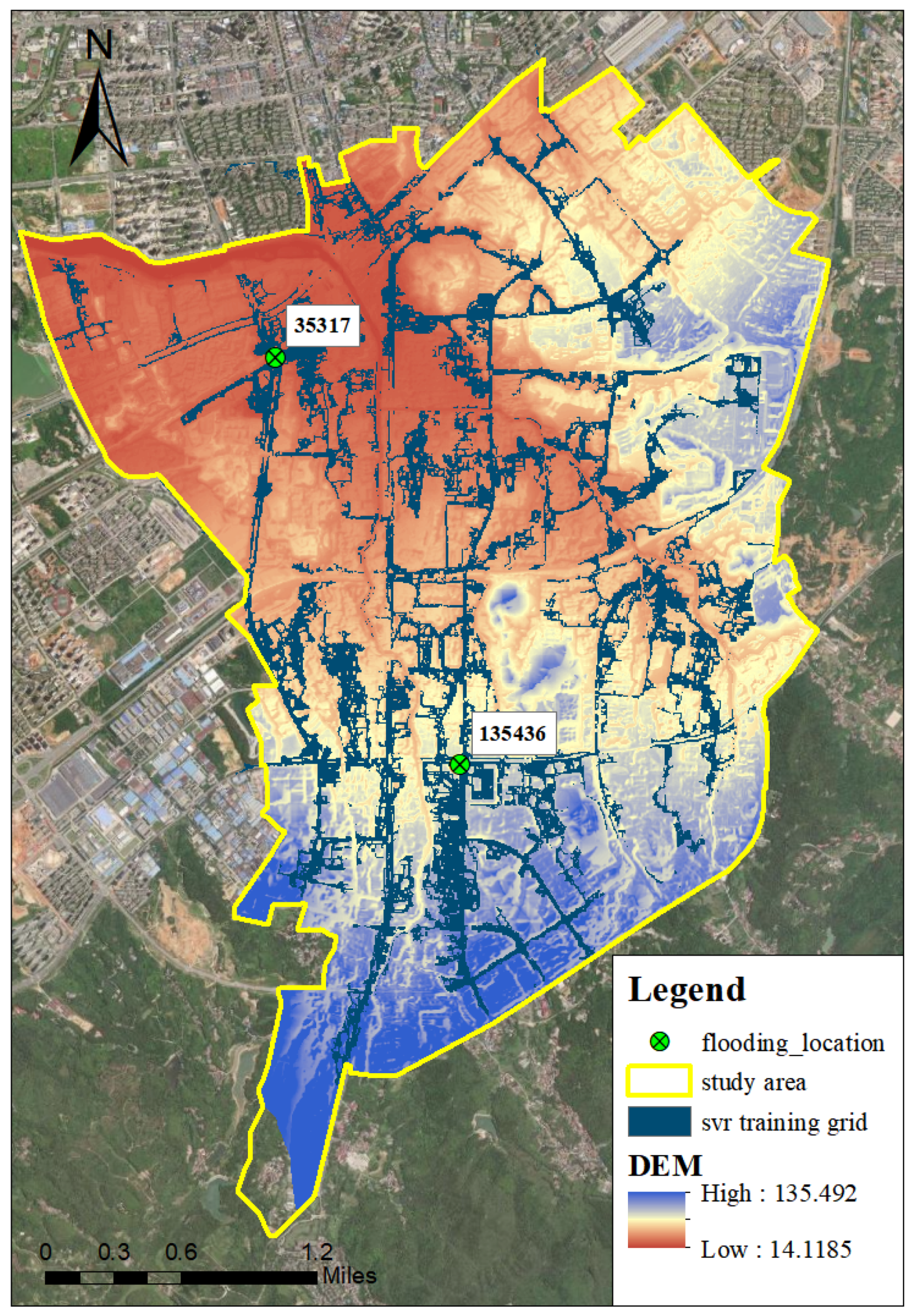
The flood maps of the max ponding depths for 3 h duration rainfall with return periods ranging from 1 to 15 years were illustrated in Figure 8. The result indicated that the study area suffered a high risk of flooding, and the main ponding locations were the places with relatively lower elevations. Therefore, a subset of 180,000 grids with ponding water was specifically selected for training purposes, and the two flooding areas were located at grids with indices 35317 and 135436, respectively, as shown in Figure 9.
Each of the selected grids was individually trained as an SVR model and used to predict the max flood water depth of this grid, and all the prediction results were eventually spliced into a max flood map. The R2 results of the grids #35317 and #135436 were derived directly from the SVR model as 0.97 and 0.98, respectively, demonstrating that the filtered features can reflect the maximum water depth well.
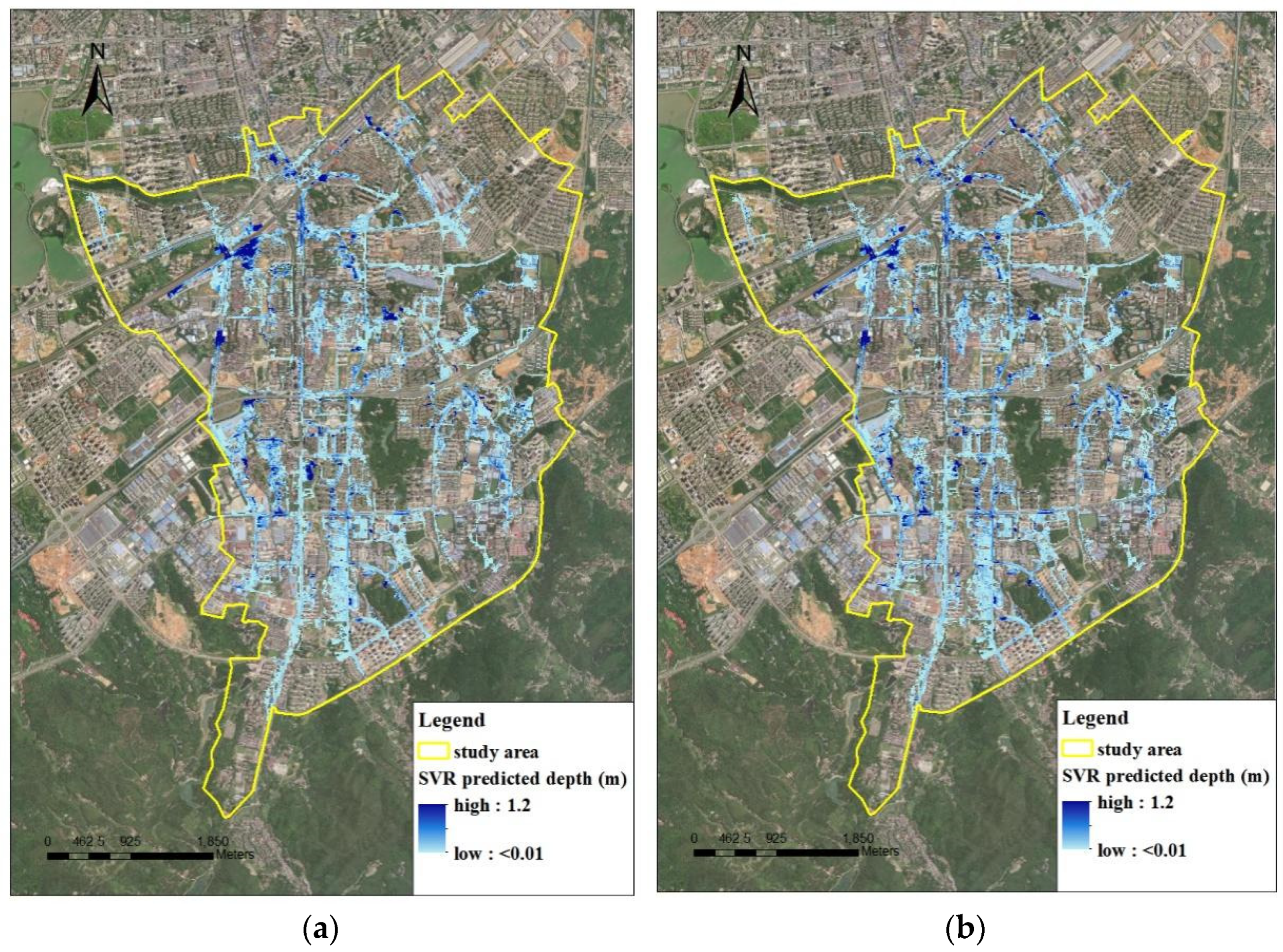
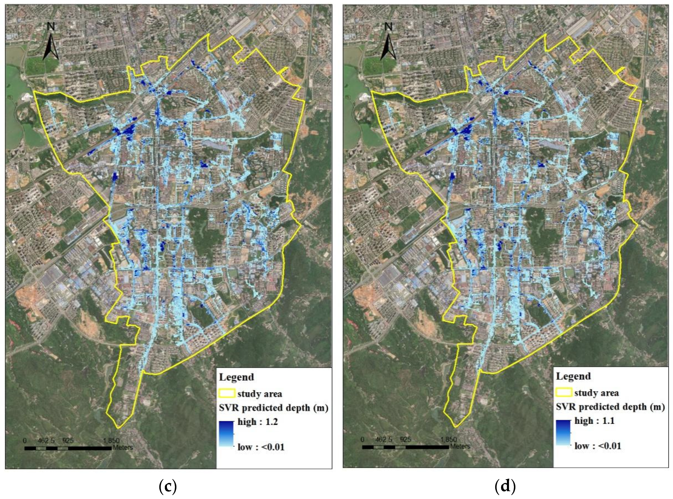
The four designed scenarios including 15-year rainfalls with durations of 1 h, 2 h, and 3 h, and 24 h cumulative rainfall of 160 mm were input into the SVR model (Figure 10 and Table 3). According to Table 3, the maximum water depth errors were all within ±1 cm, and the average relative errors was estimated to be 0.43%, indicating a high consistence between two models.
The SVR model was tested using the observed rain data from Event #3 and Event #4, obtaining an average relative error of 8.0%. The testing results deviated from reality to some extent yet were acceptable considering the precipitation error. Additionally, the influence from river water level was not included in the model. More observation data such as flooding depth and water level of river downstream were therefore required for the further study.
It was worth addressing the importance of the balance between designed scenarios and monitor data when it came to training set. The verified mechanism model represented the present hydraulic performance, yet the historical monitor values before the possible construction might mislead the model from the reality. From this point of view, the reliable mechanism model was still of great significance in the prediction procedure.

5.3. Comparison between the Mechanism Model and SVR Model

The coupled mechanism model and SVR model were run on the same environment (Intel® Core (TM) i5-10600 CPU @ 3.30GHz, 16GRAM) in order to compare their simulation time of Event #3 and #4, as presented in Table 2. The time cost by the coupled model was relatively short compared to other 2D flood software V1.0 (Table 4) but still 24 times that of the SVR model for 5 h simulation. The SVR model took approximately 1.0 min regardless of the duration of the rainfall events, as the model input was not time series but its characteristics. In other words, 1.0 min was the total time for a set of nearly 180,000 SVR models, which could be reduced by decreasing the number of grids [19].
Since the rainfall forecasting from, e.g., radar might vary extreme rapidly before and during the event, the significantly enhanced calculation efficiency by SVR model was a guarantee for spontaneous prediction each time the rain data changes.

5.4. Limitations

As mentioned, the contributions of simulations and observations in ML training set was the key consideration of forecast, which reflected the current (mechanism model) and the past (monitoring) hydraulic performance, respectively. The monitoring data thereby had to be filtered along with the pipeline maintenance and construction. This balance should be discussed and compared further when more recorded ponding events are available.
Constrained by the actual drainage system in Lianghe, features such as the upstream controlling structures (weirs, pumps, storages) and river water levels were simplified and exclusive in this case study, which might be crucial while applying this procedure in other system.
The method of choosing training and predicting grids was relatively rough in this study. The amount of selected grids determined the average ML forecast time cost. More detailed criteria could be explored to minimize the ponding area and consequently decreasing the time cost.

6. Conclusions

This study developed a coupled mechanistic flood model using the SWMM and LISFLOOD-FP models. The combined applications of the two-dimensional shallow water equation, the orifice/weir flow formula, etc., enabled an integrating calculation of the water exchange between the 1D and 2D models. This presented flood model was employed after calibration and validation to provide training data for SVR model predicting ponding in time. IDW interpolation method was applied to obtain precipitation data from various rain gauges for each elevated grid and its characteristics as max intensity (mm/5 min), accumulated volume (mm) and duration (h) were determined to be the features of SVR model. The outcome of SVR model as max depth during raining was testified by 2 monitored rainfall events, with a mean absolute error of 8.2%. This method benefitted a rapid calculation for ponding prediction, costing 1.0 min for 5 h simulation, saving 95% of the time for responses to spontaneous and emergency flooding events.
It could be widely applied to generate a flood map spontaneously for the integrating water system. The ML model had to be in sync with the system maintenances and constructions by selecting suitable monitoring data and set an acceptable ratio of monitoring and simulation contributing to training data. The model should be explored further by taking more features into account including the controlling structures, the river water level, etc., and the outcomes could be expanded to be in a time series format as a more feasible solution for practices.

Author Contributions

Conceptualization, Z.G. and X.L.; methodology, R.C.; software, M.G.; validation, Z.G.; formal analysis, Z.G.; investigation, Z.G.; resources, R.C.; data curation, M.G.; writing—original draft preparation, Z.G.; writing—review and editing, X.L.; visualization, X.W.; supervision, X.L.; project administration, X.L.; funding acquisition, R.C. All authors have read and agreed to the published version of the manuscript.

Funding

This research was funded by the Research Project of Shanghai Investigation Design and Research Institute Co., Ltd., grant number 2021QT(8)-012, Mine Temporal and Spatial Information and Ecological Restoration Key Laboratory of Ministry of Natural Resources Open fund, grant number KLM202304.

Data Availability Statement

The data presented in this study are available on request from the corresponding author.

Conflicts of Interest

Zhong Gao was employed by Shanghai Investigation, Design & Research Institute Co., Ltd. Ruihong Chen and Minrui Guo were employed by Three Gorges Smart Water Technology Co., Ltd. The remaining authors declare that the research was conducted in the absence of any commercial or financial relationships that could be construed as a potential conflict of interest.

References

  1. Chen, Y.; Han, D. Big Data and Hydroinformatics. J. Hydroinform. 2016, 18, 599–614. [Google Scholar] [CrossRef]
  2. Akter, S.; Wamba, S.F. Big Data and Disaster Management: A Systematic Review and Agenda for Future Research. Ann. Oper. Res. 2019, 283, 939–959. [Google Scholar] [CrossRef]
  3. Zhou, L.; Huang, H.; Muthu, B.A.; Sivaparthipan, C.B. Design of Internet of Things and Big Data Analytics-Based Disaster Risk Management. Soft Comput. 2021, 25, 12415–12427. [Google Scholar] [CrossRef]
  4. Martínez–Álvarez, F.; Morales–Esteban, A. Big Data and Natural Disasters: New Approaches for Spatial and Temporal Massive Data Analysis. Comput. Geosci. 2019, 129, 38–39. [Google Scholar] [CrossRef]
  5. Pedrozo-Acuña, A.; Moreno, G.; Mejía-Estrada, P.; Paredes-Victoria, P.; Breña-Naranjo, J.A.; Meza, C. Integrated Approach to Determine Highway Flooding and Critical Points of Drainage. Transp. Res. Part. D Transp. Environ. 2017, 50, 182–191. [Google Scholar] [CrossRef]
  6. Mignot, E.; Paquier, A.; Haider, S. Modeling Floods in a Dense Urban Area Using 2D Shallow Water Equations. J. Hydrol. 2006, 327, 186–199. [Google Scholar] [CrossRef]
  7. Douinot, A.; Roux, H.; Garambois, P.-A.; Larnier, K.; Labat, D.; Dartus, D. Accounting for Rainfall Systematic Spatial Variability in Flash Flood Forecasting. J. Hydrol. 2016, 541, 359–370. [Google Scholar] [CrossRef]
  8. Payande, A.R.; Niksokhan, M.H.; Naserian, H. Tsunami Hazard Assessment of Chabahar Bay Related to Megathrust Seismogenic Potential of the Makran Subduction Zone. Nat. Hazards 2015, 76, 161–176. [Google Scholar] [CrossRef]
  9. Papaioannou, G.; Loukas, A.; Vasiliades, L.; Aronica, G.T. Flood Inundation Mapping Sensitivity to Riverine Spatial Resolution and Modelling Approach. Nat. Hazards 2016, 83, 117–132. [Google Scholar] [CrossRef]
  10. Chang, X.; Xu, Z.; Zhao, G.; Du, L. Urban rainfall-runoff simulations and assessment of low impact development facilities using SWMM model-A case study of Qinghe catchment in Beijing. J. Hydroelectr. Eng. 2016, 35, 84–93. [Google Scholar] [CrossRef]
  11. Huang, G.; Huang, W.; Zhang, L.; Chen, W.; Feng, J. Simulation of rainstorm waterlogging in urban areas based on GIS and SWMM model. J. Water Resour. Water Eng. 2015, 26, 1–6. [Google Scholar] [CrossRef]
  12. Ma, R.; Bai, T.; Huang, Q.; Yang, W. MIKE 21 model and its application on urban waterlogging simulation. J. Nat. Disasters 2017, 26, 172–179. [Google Scholar] [CrossRef]
  13. Guo, F.; Qu, H.; Zeng, H.; Cong, S.; Geng, X. Flood Routing Numerical Simulation of Flood Storage Area Based on MIKE21 FM Model. Water Resour. Power 2013, 31, 34–37. [Google Scholar]
  14. Wei, K.; Liang, Z.; Wang, J. Flood Routing Simulation of MengWa Detention Basin based on MIKE21. South-North Water Transf. Water Sci. Technol. 2013, 11, 16–19. [Google Scholar] [CrossRef]
  15. Wang, X.; Han, H.; Li, H. Flood Risk and Duration Analysis of Ningjinbo and Daluze Flood Storage.detention District. Water Resour. Power 2013, 31, 59–62. [Google Scholar]
  16. Zheng, S.; Wan, Q.; Jia, M. Short-term forecasting of waterlogging at urban storm-waterlogging monitoring sites based on STARMA model. Prog. Geogr. 2014, 33, 949–957. [Google Scholar] [CrossRef]
  17. Li, X.-L.; Lü, H.; Horton, R.; An, T.; Yu, Z. Real-Time Flood Forecast Using the Coupling Support Vector Machine and Data Assimilation Method. J. Hydroinform. 2013, 16, 973–988. [Google Scholar] [CrossRef]
  18. Abou Rjeily, Y.; Abbas, O.; Sadek, M.; Shahrour, I.; Hage Chehade, F. Flood Forecasting within Urban Drainage Systems Using NARX Neural Network. Water Sci. Technol. 2017, 76, 2401–2412. [Google Scholar] [CrossRef] [PubMed]
  19. Yan, J.; Jin, J.; Chen, F.; Yu, G.; Yin, H.; Wang, W. Urban Flash Flood Forecast Using Support Vector Machine and Numerical Simulation. J. Hydroinform. 2017, 20, 221–231. [Google Scholar] [CrossRef]
  20. Chen, W. Urban Flood Hydrological and Hydrodynamic ModelConstruction and Flood Management Key Issues Exploration; South China University of Technology: Guangzhou, China, 2020. [Google Scholar] [CrossRef]
  21. Legates, D.R.; McCabe, G.J., Jr. Evaluating the Use of “Goodness-of-Fit” Measures in Hydrologic and Hydroclimatic Model Validation. Water Resour. Res. 1999, 35, 233–241. [Google Scholar] [CrossRef]
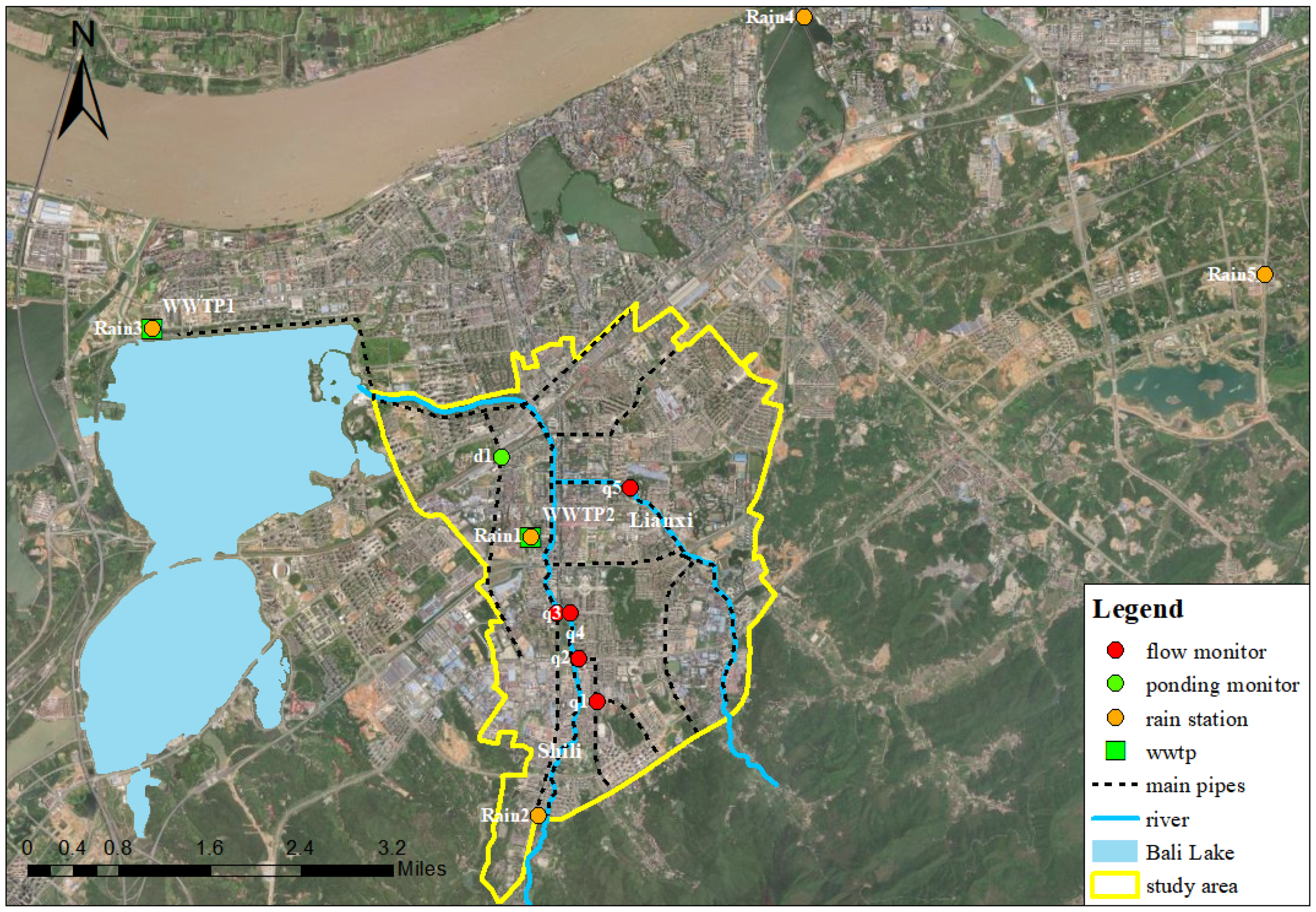
Figure 1. The study area and implemented monitors.
Water 16 01694 g001
Figure 2. The modelling area and two primary flooding locations.
Water 16 01694 g002
Figure 3. Flow chart of applied methodology.
Water 16 01694 g003
Figure 4. Schematic diagram of junction outflow (left) and surcharged flow (right).
Water 16 01694 g004
Figure 5. Sketched SWMM model layout of drainage system and rivers in Lianghe. (a) Drainage system; (b) rivers; (c) integrating 1D model of drainage system and rivers.
Water 16 01694 g005
Figure 6. Calibration (left) and validation (right) results of the 1D SWMM model.
Water 16 01694 g006
Figure 7. Calibration (up) and validation (down) results of the coupled flood model.
Water 16 01694 g007
Figure 8. Flood maps of Lianghe generated by the coupled model under (a) the designed 3 h 1a rainfall, (b) the designed 3 h 2a rainfall, (c) the designed 3 h 3a rainfall, and (d) the designed 3 h 5a rainfall.
Water 16 01694 g008aWater 16 01694 g008b
Figure 9. Selected training grids for the SVR model and the flooding location index.
Water 16 01694 g009
Figure 10. Flood maps of Lianghe generated by the SVR model under (a) the designed 1h 15a rainfall, (b) the designed 2 h 15a rainfall, (c) the designed 3 h 15a rainfall, (d) the designed 24 h 160 mm rainfall.
Water 16 01694 g010aWater 16 01694 g010b
Table 1. The summarized information of precipitation events for model calibration and verification.
TimeTotal Rainfall Amount at Station 1 (mm)Total Rainfall Amount at Station 2 (mm)Available MonitorsUsageRain EventRainfall Duration (h)
1#5 June 2023 5:15–5 June 2023 6:253124q1, q2, q3, q4 *SWMM model verification, SVR model training1#2.1
2#22 June 2023 14:35–26 June 2023 7:5510099q2, q3, q4, q5 **SWMM model calibration,
SVR model training
2#142
2#215
2#318
3#22 July 2023 9:30–22 July 2023 14:303421d1Coupled model verification, SVR model validation3#4.7
4#21 August 2023 19: 30–28 August 2023 4:204437d1Coupled model calibration, SVR model validation4#8.8
Notes: * Monitor q5 was not implemented until event 2#. ** Monitor q1 was out of function during event 2# due to signal failure.
Table 2. Designed scenarios for SVR model training and validation.
TypeDuration (h)Return Period (a)Accumulated Rainfall (mm)Number
1115 * 1
2215 *20, 30, 50, 1005
330.05, 0.1, 0.2, 0.3, 0.5, 1, 2, 3, 5, 10, 15 *, 20, 30, 50, 100 15
424 30, 50, 100, 150, 160 *6
Note: * events used for model validation.
Table 3. Comparison of maximum ponding depth calculated by machine learning model and mechanism model.
NumberEventsObserved/Coupled Model Result Max Ponding Depth at d1 (m)SVR Result Max Ponding Depth at d1 (m)Percentage Error
1Design rainfall, 1 h, 15a (74 mm)1.21.2 <0.01%
2Design rainfall, 2 h, 15a (92 mm)1.21.2 <0.01%
3Design rainfall, 3 h, 15a (105 mm)1.21.2 <0.01%
4Design rainfall, 24 h, 160 mm1.11.1 <0.01%
5Observed rainfall, 4.67 h, 34 mm (Rain1) (event #3)1.41.716%
6Observed rainfall, 8.75 h, 43.5 mm (Rain1) (event #4)1.61.6 <0.01%
Table 4. Comparison of maximum ponding depth calculated by machine learning model and mechanism model.
ModelSimulation Time for Event #3 (8 h)Simulation Time for Event #4 (5 h)
The coupled mechanism model38 min24 min
The SVR model1.0 min1.0 min
Disclaimer/Publisher’s Note: The statements, opinions and data contained in all publications are solely those of the individual author(s) and contributor(s) and not of MDPI and/or the editor(s). MDPI and/or the editor(s) disclaim responsibility for any injury to people or property resulting from any ideas, methods, instructions or products referred to in the content.