Article

Artificial Neural Network (ANN)-Based Water Quality Index (WQI) for Assessing Spatiotemporal Trends in Surface Water Quality—A Case Study of South African River Basins

by
Talent Diotrefe Banda
1,* and
Muthukrishnavellaisamy Kumarasamy
1,2
1
Department of Civil Engineering, School of Engineering, College of Agriculture, Engineering and Science, University of KwaZulu-Natal, Howard College, Durban 4041, South Africa
2
Saveetha School of Engineering, Saveetha Institute of Medical and Technical Sciences, Chennai 600072, India
*
Author to whom correspondence should be addressed.
Water 2024, 16(11), 1485; https://doi.org/10.3390/w16111485
Submission received: 25 April 2024 / Revised: 12 May 2024 / Accepted: 21 May 2024 / Published: 23 May 2024
(This article belongs to the Section Water Quality and Contamination)

Abstract

:
Artificial neural networks (ANNs) are powerful data-oriented “black-box” algorithms capable of assessing and delineating linear and multifaceted non-linear correlations between the dependent and explanatory variables. Through the years, neural networks have proven to be effective and robust analytical techniques for establishing artificial intelligence-based tools for modelling, estimating, and projecting spatial and temporal variations in water bodies. Accordingly, ANN-based algorithms gained increased attention and have emerged as practical alternatives to traditional approaches for hydro-chemical analysis. ANNs are among the widely used computer systems for modelling surface water quality. Considering their wide recognition, resilience, flexibility, and accuracy, the current study employs a neural network-based methodology to construct a novel water quality index (WQI) model suitable for analysing South African rivers. The feed-forward, back-propagated multilayered perceptron model has three parallel-distributed neuron layers interconnected with seventy weighted links orientated laterally from left to right. First, the input layer includes thirteen neuro-nodes symbolising thirteen explanatory variables, including NH3, Ca, Cl, Chl-a, EC, F, CaCO3, Mg, Mn, NO3, pH, SO4, and turbidity (NTU). Second, the hidden layer consists of eleven neuro-nodes accountable for computational tasks. Lastly, the output layer features one neuron responsible for conveying network outcomes using a single-digit WQI rating extending from zero to one hundred, where zero represents substandard water quality and one hundred denotes exceptional water quality. The AI-based model was developed using water quality data obtained from six monitoring locations within four drainage basins under the management of the Umgeni Water Board in the KwaZulu-Natal Province of South Africa. The dataset comprises 416 samples randomly divided into training, testing, and validation sets using a proportional split of 70:15:15%. The Broyden–Fletcher–Goldfarb–Shanno (BFGS) technique was utilised to conduct backpropagation training and adjust synapse weights. The dependent variables are the WQI scores from the universal water quality index (UWQI) model developed specifically for South African river basins. The ANN demonstrated enhanced efficiency through an overall correlation coefficient (R) of 0.985. Furthermore, the neural network attained R-values of 0.987, 0.992, and 0.977 for the training, testing, and validation intervals. The ANN model achieved a Nash–Sutcliffe efficiency (NSE) value of 0.974 and coefficient of determination (R2) of 0.970. Sensitivity analysis provided additional validation of the preparedness and computational competence of the ANN model. The typical target-to-output error tolerance for the ANN model is 0.242, demonstrating an adequate predictive ability to deliver results comparable with the target UWQI, having the lowest and highest index ratings of 75.995 and 94.420, respectively. Accordingly, the three-layer neural network is scientifically sound, with index values and water quality evaluations corresponding to the UWQI results. The current research project seeks to document the processes used and the outcomes obtained.

1. Introduction

Artificial intelligence (AI), specifically, the artificial neural network (ANN), has become popular for assessing surface water quality [1,2]. Developing AI-based models is less taxing than establishing conventional and statistically developed water quality indices involving sub-index functions and aggregation equations [3]. Therefore, ANNs are convenient and straightforward techniques for assessing water quality, potentially reducing computational oversights, time spent, and effort necessary for evaluating water bodies [3,4,5]. Neural networks use mathematical coding that symbolises predetermined multidimensional variable relationships [6,7,8,9,10,11,12]. Their capacity to comprehend and relate to variable dependency offers a distinct computational superiority and yields more precise WQI ratings than sub-indexing methodologies [13,14]. Like the human brain cortex, ANNs operate using analytical systems based on the structure and functionality of the biological neural configurations. They function identically to human brains in analysing and processing information, with layers of neurons intertwined, forming a complex web [1,6,7,10,11,15,16,17,18,19,20,21]. The initial layer comprises neurons that input information and seek to assess the data before filtering them to the appropriate neural cells in the subsequent layer. The second layer contains neurons responsible for processing the incoming data and transmits the findings to the third layer of neurons, which combines everything into a single aggregated output report. These computational cells are called neuro-nodes or input and output units [4,22,23].
ANNs are basic non-linear statistical algorithms used to improve artificial intelligence (AI) and address data-driven challenges that are difficult or impractical to manage using human or mathematical methods [7,8,10,11,12,15,22,24]. ANNs are transforming conventional technologies to evaluate water quality indices, thus developing convenient analytical platforms while making water quality data readily available with little effort. This research establishes an artificial neural network-based water quality index (WQI) for evaluating spatial and temporal changes in surface water across South African river basins.
The ANN model employs thirteen parameters that are identical to the input variables of the universal water quality index (UWQI), namely NH3, Cl, Chl-a, EC, F, CaCO3, Mg, Mn, NO3, pH, SO4, and turbidity. The AI-based model generates a scientifically sound non-dimensional one-digit rating varying from zero to one hundred, with smaller ratings representing poor water quality and larger scores representing excellent water bodies. Index scores are assessed on a five-class scale, with Class 1 indicating the greatest degree of cleanliness and Class 5 indicating severely polluted water resources. The WQI values and ranking scale are comparable and conform to the gradings established using the UWQI and surrogate water quality index (proxy WQI), both used for appraising South African rivers [25,26,27].
Generally, WQIs are not designed for broad application; they are customarily developed for a specific watershed and/or region, unless different basins share similar attributes and test comparable ranges of water quality parameters. Their design and formation are governed by the intended use together with the degree of accuracy required, and such technicalities ultimately define the application boundaries of WQIs [26]. This is, perhaps, the most demanding scientific need; that is, to establish a universal water quality index (UWQI), that can function in most, if not all, the catchments in South Africa. The challenges posed by developing universal WQI models include the selection of the most appropriate variables applicable across all targeted catchment areas. Accordingly, this study derived thirteen parameters using expert opinion gathered through the participatory-based Delphi method [3,28,29,30,31,32,33,34,35] and extracted from previously published studies; these results were published separately as Banda and Kumarasamy [27]. In cognisance of such, this study proposes an index that is not limited to certain application boundaries, and such a contribution significantly contributes to the field of water science and the South African community. Hence, the aims of developing ANN models in this study include (i) demonstrating the application of artificial intelligence (AI) in water management and the use of universal WQIs using an ANN-based WQI without sub-indexing and extensive calculations; (ii) establishing an overall framework for developing neural networks; (iii) comparing the effectiveness of the ANN model with the traditional WQI; and (iv) suggesting the ideal artificial neural network WQI model for evaluating and tracking water quality status throughout South African river catchments. Accordingly, this research discusses the design, training, validation, testing, and implementation of ANNs to formulate WQI ratings.

2. Materials and Methods

2.1. Research Data

Gathering historical water quality data is time-consuming and requires significant resources and proficiency [27]. Consequently, research projects, including the current study, cannot collect water quality samples. Instead, monthly water quality readings from the Umgeni Water Board (UWB) located in Durban, South Africa, enabled the development of the artificial neural network (ANN) model. This research study examined 416 sample cases collected from six monitoring points in four distinct watersheds over four years from January 2014 to July 2018. The watersheds are Umgeni, Umdloti, Nungwane, and Umzinto/Umuziwezinto river catchments. The UWB water quality records were collected using standard sampling techniques established by the Department of Water and Sanitation (DWS) and examined in an ISO 9001-recognised laboratory owned and managed by UWB [27,36]. The UWB research dataset included all thirteen essential water quality indicators, which are ammonia (NH3), calcium (Ca), chloride (Cl), chlorophyll-a (Chl-a), electrical conductivity (EC), fluoride (F), hardness (CaCO3), magnesium (Mg), manganese (Mn), nitrate (NO3), pondus Hydrogenium (pH), sulphate (SO4), and turbidity (NTU). Table 1 presents descriptive statistics of the research dataset.
Evaluating the WQI model with information gathered from these four river basins contributes to developing water quality indices appropriate for most river basins, if not the entirety of South African river catchments. Apart from the availability of UWB data, the economic importance of the KwaZulu-Natal Province [27,37,38], the uniqueness of its inter-basin configurations, the magnitude of the transfer schemes involved, and the significant water demand [27,39,40] all contributed to selecting the research area, which is located within the Pongola-Mtamvuna WMA (water management area) [41,42]. The study dataset was sufficient for evaluating the model and contributing to achieving the objective of establishing a widely acceptable water quality monitoring tool.

2.2. Sampling Stations

Umgeni Water Board (UWB) assembled water sample stations to improve water quality monitoring, and the sampling points are placed strategically to offer a comprehensive understanding of water affairs throughout the KwaZulu-Natal service region. The current research used water quality records gathered by UWB rather than building new research-based monitoring points. Consideration was given to at least one station within the four watersheds mentioned in the previous sections. The designated sampling locations are outlined in Table 2 and Figure 1. The Umgeni basin’s socioeconomic significance, the distinctive characteristics that define its inter-basin configurations, the complexity of the transfer schemes involved, and the substantial water demand necessitate comprehensive water resource administration. These factors contributed to selecting and recognising the Umgeni River basin as the primary research area. Additionally, three more basins were included in the research project to evaluate the model and support the objective of establishing a universally accepted WQI model.

2.3. Study Area

The research area is in South Africa, within the KwaZulu-Natal Province, under the management of the Umgeni Water Board, and contains four significant river catchment basins, as detailed below.

2.3.1. Umgeni River Catchment

The Umgeni River basin is a sub-humid drainage region within KwaZulu-Natal Province near the Indian Ocean shoreline east of South Africa [38,43,44]. The river catchment area is over 4432 km2, with the Umgeni River as the major watercourse within the drainage region [36,37,42,45]. The 232 km long river, starting from the Drakensberg mountains, extends eastwards into the Indian Ocean, having four primary cardinal tributaries, namely Lions, Karkloof, Impolweni, and Umsunduzi Rivers [42,44]. Lions River is the largest tributary north of Midmar Dam, operating as a transfer route supplying water from the nearby Mooi River basin [36]. The land cover in the basin is generally diversified, with urban settlements, indigenous forests, sugarcane fields, farmlands, and the Port City of Durban [36,37,38,43]. Notably, Umgeni River supplies informal settlements located along the riverbanks. They depend upon the river primarily for their domestic needs, irrigation, and livestock farming [46]. The rainfall pattern for the catchment is seasonal, with maximum rains occurring during the summertime (October to March). Precipitation fluctuates exceptionally, increasing from the west to the east of the river basin. The heaviest rainfall occurs towards the coast, measuring between 1000 and 1500 mm/yr [37,44]. The middle sections of the catchment area receive rainfall varying from 800 mm/yr to 1000 mm/yr [37,43,47].
The average yearly temperature fluctuates between 12 °C and 22 °C, resulting in evaporation rates ranging from 1567 mm/yr and 1737 mm/yr [36]. Albert Falls, Inanda, Nagle, and Midmar Dams are primarily designed to control and conserve water resources throughout the Umgeni catchment area [36,39]. The Albert Falls, Nagle, and Inanda Dams supply most of the Durban Metropolitan Area, while the Midmar Dam provides water to Pietermaritzburg and parts of Durban [42,43,44]. Apart from the four primary dams, the basin also has Henley Dam, located south of Midmar Dam along the Msunduzi River, which is a tributary of the Umgeni River. In addition, around 300 farm dams are used to irrigate approximately 185 km2 of agricultural fields within the Umgeni catchment region [25,27,43].

2.3.2. Umdloti River Catchment

The Umdloti watershed lies northeast of the Umgeni catchment, near the Nagle and Inanda dams. The catchment is estimated to measure 597 km2, with the Umdloti River being the major river within the drainage area [48]. The river’s headwaters are within the Noodberg area and descends eastwards into the Indian Ocean for roughly 88 km. The river estuary is nearly 25 km northeast of Durban City [45,49]. A substantial proportion of the basin is used for agricultural activities, with sugarcane and banana production dominating, while citrus and vegetable farms occupy minimal space. Other facilities include Verulam Town, wildlife reserves, the Hazelmere Wastewater Treatment Works (WWTW), and the Hazelmere Dam [49]. Comparable to the Umgeni basin, the Umdloti catchment receives summer rainfall, having mean annual precipitation varying from 800 mm to 1125 mm. Temperatures fluctuate between 9 °C during wintertime and 38 °C in summertime [49]. The main water retention facility in the Umdloti basin is Hazelmere Dam [48], constructed to supply Durban’s residential, commercial, and agricultural demands, together with the demands of the newly established Durban International Airport [25,27,45,49].

2.3.3. Nungwane River Catchment

Situated southwest of the Umgeni catchment area, the Nungwane River basin experiences an average rainfall of 938 mm/yr and evaporation rates reaching 1200 mm/yr. The Nungwane Dam is the largest impoundment within the quaternary catchment and was constructed along the Nungwane River, a tributary of the Lovu River [50]. The retention facility was established in 1977, having an overall catchment of 58 km2, and surface water from Nungwane Dam is purified at the Amazimtoti water treatment works (WTW) and distributed to eThekwini Municipality [25,27,50].

2.3.4. Umzinto/uMuziwezinto River Catchment

The Umzinto River basin, formerly recognised as the uMuziwezinto River catchment, is located southward of the Nungwane Dam. Corresponding to Umgeni Water [50], the Umzinto River catchment encounters about 985 mm/yr of rain, with an average evaporation rate of approximately 1200 mm/yr. In 1993, Umzinto Dam was established with a geographical catchment nearing 52 km2, and the impoundment lies along the Umzinto/uMuziwezinto River [27]. Surface water from Umzinto and EJ Smith Dams is purified at Umzinto water treatment works (WTW) and supplied to Ugu District Municipality [50,51]. Both dams, EJ Smith and Umzinto, supply raw water for the operation of Umzinto WTP [25,27,50,51].

2.4. Water Quality Evaluation

Two variables are needed when developing artificial neural networks: the explanatory (independent) and target (dependent) variables. The current research study considered the value of the water quality index (WQI) as the dependent variable, and the observed physicochemical water quality readings were regarded as the explanatory variables. WQI is a basic yet comprehensible ranking score that offers the composite influence of multiple water quality characteristics for a specific body of water [25,52,53,54]. An index number is often assessed against a ranking system that describes water quality in classifications varying between zero and one hundred [25,55]. Accordingly, the recently developed universal water quality index (UWQI) was used for WQI evaluation, and the model consists of the following components:
(1)
Explanatory variables: Thirteen preselected independent water quality indicators, namely NH3, Ca, Cl, Chl-a, EC, F, CaCO3, Mg, Mn, NO3, pH, SO4, and Turb, were adopted based on expert opinion [25,27]. The study incorporated expert opinion through the Rand Corporation’s Delphi Technique, where a panel of thirty water scientists from the private sector, government institutions, and academia were consulted. Delphi Questionnaires were distributed to water specialists (the participants), and the panellists were requested to select about twenty-one water quality indicators for potential inclusion in the UWQI. The respondents were directed to decide on each parameter using: “Include” and “Exclude” and further designate a proportional significance ranking for each parameter specified as “Include”. The ranking system utilised is scaled from one to five, with “scale 1” indicating the highest significance and “scale 5” indicating an exceptionally low relevance. Apart from the twenty-one indicators specified, professionals could include up to five additional parameters where necessary. Amongst the thirty questionnaires distributed, a total of twenty-one surveys were returned. The Rand Corporation’s Delphi Technique is comprehensively discussed by Horton [28], Brown et al. [29], Linstone and Turoff [30,33], and Gazzaz et al. [3].
(2)
Weighting coefficients: Weight multipliers (bi) starting from one (relating to minimum impact) and extending to five (resembling maximum impact) were allocated to each variable after aggregating significance rankings obtained from the participatory-based Delphi approach, together with significance rankings drawn from the existing literature. After that, weighting coefficients (wi) were derived using Equation (1) below [25,27,56]:
w i = b i ( b 1 + b 2 + + b n )  
where bi denotes the designated significance ranking of the ith water quality variable (one being the lowest order ranking and five the highest order); wi represents the weighted coefficient for the ith water quality variable in decimal digits; and n symbolises the sum of the rated water quality variables. The coefficients are expressed in decimal format, and the aggregate of all weighting coefficients equals one. This criterion guarantees that the final index score does not surpass 100% (w1 + w2 + w3 + … + wn = 1 for Equation (1)). Otherwise, the sub-indexing system will be jeopardised, making the WQI model dysfunctional. The final weighting coefficients are presented in Table 3.
(3)
Sub-index functions and rating curves: Given that water quality indicators are measured using several scientific units, sub-indices (si) are employed to transform multiple units of measurement into one conventional non-dimensional scale [25,57]. Using sub-indices to transfigure multiple parameter dimensions is standard practice, and the traditional method includes sub-index rating curves, which are then converted into mathematical equations called sub-indices. In this case, the designated key points that define the rating curves are geometrically established using the permitted concentration limits. After that, straight-line plots are utilised to converge the mapped points and generate a sequence of linear graphs, which are then transformed into linear sub-index equations (index functions). The study extracted permissible concentration limits from the Target Water Quality Ranges (TWQRs) documented by the Department of Water and Sanitation (DWS), formerly the Department of Water Affairs and Forestry (DWAF) [58,59,60],
(4)
Aggregation equation (model): The UWQI model represents a weighted arithmetic sum model, a modified form of the weighted sum algorithm. As indicated in Equation (2) [25,27], the scenario-based analysis was implemented to adjust and synchronise the index algorithm with local conditions and establish the final UWQI model:
UWQI = 2 3 i = 1 n s i w i 1.0880563
where UWQI represents the final aggregated water quality index score extending from zero to hundred, with zero denoting poor water quality and hundred showing excellent water quality; si designates the sub-index value for the ith water quality variable formulated using the sub-index linear equations or functions, and the values vary between zero and one hundred, similar to WQI scores; wi is the weighting coefficient value for the ith variable expressed as a decimal figure, and the aggregate of all weight coefficients equals one, (w1 + w2 + w3 + … + wn = 1); n symbolises the overall number of sub-indices, and for the current study n = 13. WQI values are communicated as numerical digits varying between 0 and 100, where zero signifies poor water quality, and one hundred denotes excellent water quality.
Summaries of the index scores and sixty-two sub-index functions for the UWQI are presented in Figure 2 and Table 4, respectively.

2.5. Water Classification

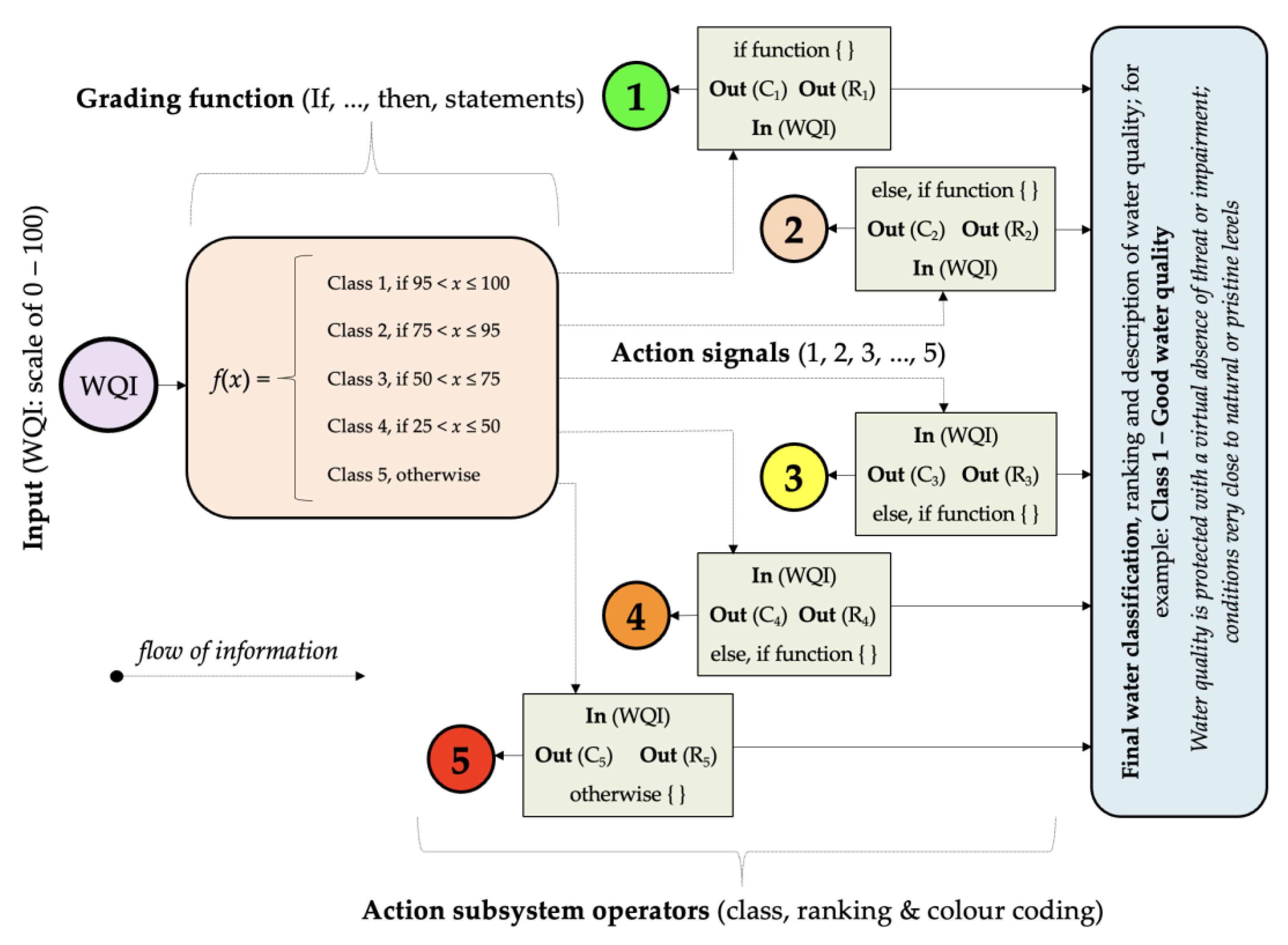
A five-class ranking system was established to classify water quality index (WQI) scores and simplify the understanding of WQI values, especially for non-technical individuals. The categorisation schema follows an increasing scale index like the normal percentage hierarchy [27,56], which is familiar to the public in terms of both functionality and interpretation. Both WQI models applicable to the current research study yield WQI scores between zero and one hundred. Consequently, the water classification schema comprises five ranks ranging from one to five, where “Class 1” designates water with the highest possible WQI score of hundred and, vice versa, “Class 5” represents water quality with the lowest index scores nearing or equal to zero. To address flaws identified in some of the existing water classification ranking systems [27,57], relevant mathematical functions with logical linguistic descriptors, including but not limited to “greater than”, “less than”, and “equal to”, are applied to appraise WQI ratings and appropriately designate them to the matching category [25,27].

2.6. Artificial Neural Network (ANN) Model

2.6.1. The ANN Model Optimisation and Structure

The artificial neural network (ANN) model, which corresponds to the universal water quality index (UWQI), was built using an identical combination of input parameters constituting the UWQI model. Against this background, the thirteen input variables were examined and processed using specified multidimensional parameter relationships established as mathematical codes. The technique is comparable to the structure and characteristics of the natural human brain [6,7,10,11,15,16,17,18,19,20,21], where multiple layers of neurons are linked together through a web-like pattern and interact from one layer to the other based on the information received and the anticipated outcome. Equally, the ANN architecture constitutes nineteen neuro-nodes and seventy synapses called “channels”, which translate several water quality indicators and integrate them into a single non-dimensional numeric rating indicating the cleanliness of water resources.
The suggested neural network model has multiple layers linked using channel links containing different weights. These layers are organised as follows: (1) an input layer that receives external information, (2) hidden or “zero” layers that seek to evaluate the input data and transmit them to the appropriate neurons in the subsequent layer, and (3) an output layer that merges the findings into one consolidated output report. The hidden layers are situated between the input and output layers [9]. Nevertheless, ANN algorithms are characterised as “black-box models” since they provide little insight regarding the influence of each parameter on the overall index value [8,10]. However, these machine learning tools are robust, relatively straightforward, non-linear statistical systems that augment artificial intelligence (AI) and address seemingly impossible tasks [8,11,13,18,24,62]; consequently, neural networks are commonly called “universal function approximators”.
There is no specific method for establishing the optimal numbers of layers and neuro-nodes; rather, the best neural network arrangement is determined by several factors [17]. According to the literature [3,7,9,17], having excessive layers in neural network models is frequently linked with “over-fitting” challenges and rarely provides ideal prediction performance. Consequently, the current research focused on three-layer artificial neural networks having input, hidden, and output layers. The exact number of neurons necessary to achieve optimal performance varies depending on the problem under consideration [6,9]. Input and output neuro-nodes are frequently specified depending on the array of input variables examined and the desired output of the neural network. Neuro-nodes in the hidden or “zero” layer are the model’s fundamental computational units, and maximising the number of such neural cells is crucial to the models’ functionality. Limiting the neuro-nodes may prevent the network from learning effectively. However, a disproportionate number of hidden nodes could cause the learning procedure to be prolonged, resulting in data “over-fitting” [6,7,9,17].
In order to establish the optimal number of hidden layers and prevent over-fitting, Fletcher and Goss [63] recommended that hidden or “zero” layer neuro-nodes (Hnod) vary from 2(Inod)0.5 + Onod to 2Inod + 1, where Inod and Onod represent the overall number of input and output neurons, respectively [6,9]. Nonetheless, Alyuda Research Inc. [64] indicated that the Hnod range extends from 0.5Inod to 4Inod. Palani et al. [65] proposed that Hnod could extend from Inod to 2Inod + 1; however, Hnod should not fall beneath 0.333Inod and Onod [3]. Most recently, García-Alba et al. [4] suggested that hidden layer neuro-nodes (Hnod) should not exceed twice the number of input nodes (Inod) and submitted the following Equation (3) [4]:
0.5Inod − 2 ≤ Hnod ≤ 2Inod + 2

2.6.2. Activation Functions and Learning Procedure

The activation functions are accountable for activating the perceptron, depending on the higher weight. Four activation functions, namely (1) tanh, (2) exponential, (3) logistic-sigmoidal, and (4) identity function, were investigated. Eventually, the logistic function, most recognised as the sigmoid activation function, performed better with the suggested neural network architecture across the hidden and output layers.
When the sum of weights and bias constant (∑xiwi + bi) is higher or equivalent to 0.5, the sigmoid function activates the neuro-node; alternatively, the neuron remains inactivated. Values < 0.5 are translated to zero, and the neuron remains dormant. In contrast, values ≥ 0.5 are turned to one, and the neuron becomes active and transmits water quality data to the next appropriate neuron. Figure 3 and Equation (4) illustrate the logistic function [4,15,65]. The sigmoid function represents a widespread activation function for artificial neural networks; nonetheless, the sigmoid function suffers from saturation problems. Thus, greater sigmoidal values snap to one, while lower digits collapse to zero. Additionally, the sigmoid-activated function is susceptible to variations at the midpoint. Despite this, the logistic-sigmoidal function was demonstrated to be the best activation function for the suggested artificial neural network. Empirical water quality records are frequently connected with parameters containing distinct measurement units, making the process cumbersome and perhaps resulting in measurement errors, noise, or interference [3,15,19]. Such effects may transmit negative inputs during network learning since specific ANN training algorithms are inconsistent with diversified data units. Because of this, the research project considered standardising the real-time water quality parameter measurements to correspond with the logistic-sigmoidal units varying between zero and one. The method prevents parameters from inappropriately influencing neural network operations [3,15,66].
sigmoid   function :   f ( z ) =   1 1 + e z  
where :   z = i = 1 n   w i x i + b i
Essentially, machine learning is performed to develop neural networks with excellent approximation ability, which can be measured using a variety of statistical attributes. A predefined training terminating criterion should be applied to guide and conclude the learning process to avoid overtraining or over-fitting and enhance applicability [6]. For this research, four stopping strategies were recommended, namely:
(a)
Whenever the cross-validation subset becomes static or starts to increase, terminate the learning cycle [3,67];
(b)
When the minimal reduction in error is approximately 0.0000001 [3];
(c)
When the mean-squared error margin on the training subset equals 0.010 [3]; and
(d)
When the learning reaches the maximum of ten thousand iterations [3].
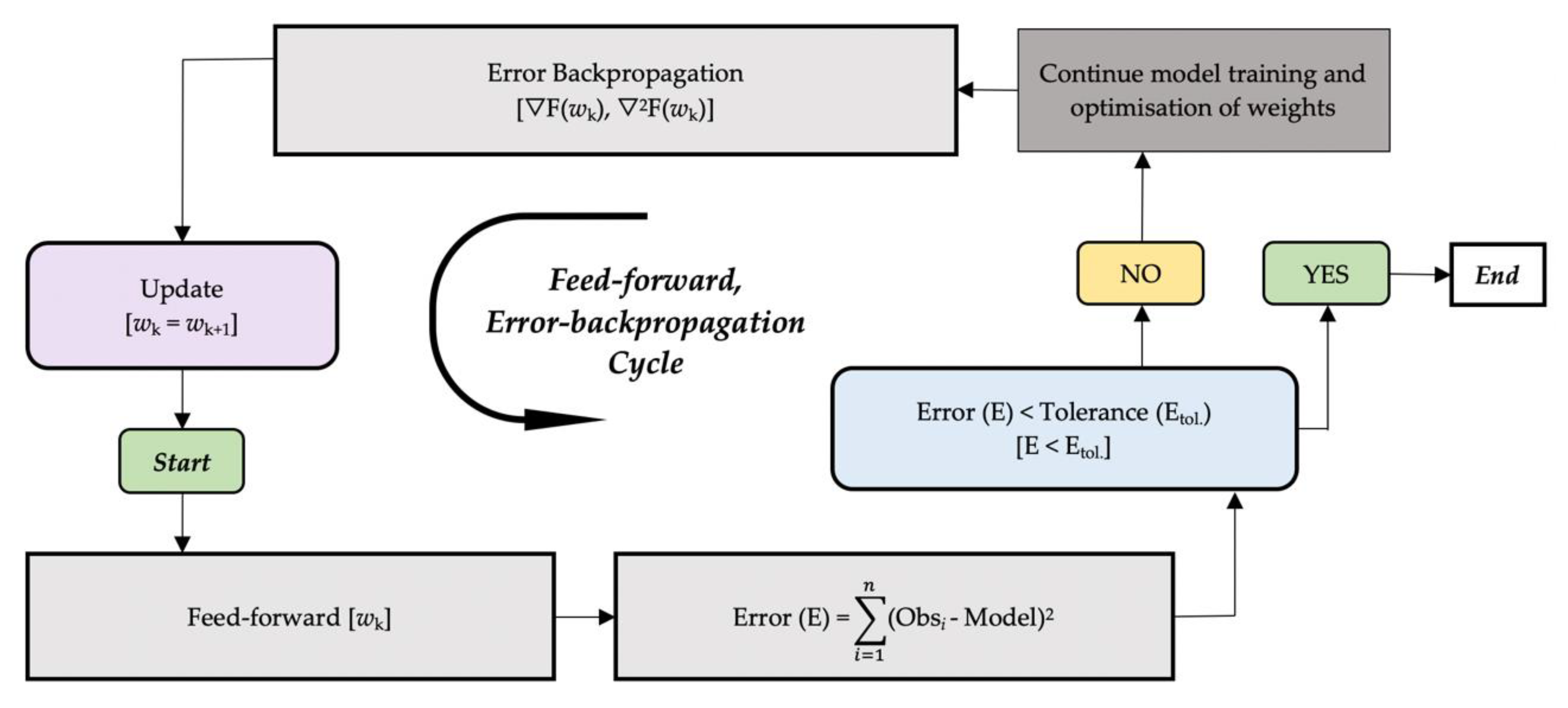
The neural network’s training procedure was conducted using backpropagation procedures [20,66], and the water quality input dataset was randomly divided to generate data subsets for training (70%), testing (15%), and validation (15%) [4,17,19,66,68,69,70,71,72,73]. Splitting the data guarantees that the predictive algorithm uses different datasets for every learning activity. Training data were used for pattern recognition, establishing neuron activation functions, and optimising hidden layer neuro-nodes, synapse weights, and bias constants. The generalisation capacity of the neural network was examined using the testing data subset, while the predictive ability was measured through validation data [20]. The learning procedure was managed and terminated through established stopping guidelines to prevent over-fitting [6,7,9,17]. The parameter measurement units were standardised, creating a uniform non-dimensional scale with values ranging between zero and one. This method helps prevent the impact of multiple measurement scales and prohibits specific variables from unreasonably dominating the modelling process [3,15,66]. The feed-forward procedure and the backward propagation of errors procedure are used for machine learning, and the techniques are discussed further in the following subsections.
The Forward Propagation Procedure: Provided that f(xi) designates the input variable, wi represents the weight coefficient for the channel link (synapse), and bij denotes the bias constant of the neuro-node, then, the feed-forward procedure is interpreted as follows [4,6,7,10,15,16,18,66,74,75]:
(i)
First Step—data inputting: f(xi) accepts as an input variable to the relevant neuron within the first layer of the artificial neural network (x1, x2, …, xn).
(ii)
Second Step—data transmission: Transfer or feed through channel links to the next layer of neurons, and the synapses are designated with relative coefficients called weights (wij).
(iii)
Third Step—application of weighting coefficients: Inputs received in the first layer are adjusted using the relative numeric weight coefficients and considered as input to the next cluster of neuro-nodes in the hidden layer (x1w1 + x2x2 + … + xnwn) = (∑xiwi).
(iv)
Fourth Step—application of bias constants and activation functions: Every hidden layer neuro-node is assigned a numeric constant called bias (b1, b2, …, bn), which is added to the input sum (∑xiwi + bi). Subsequently, the information passes through a threshold function, namely the activation function, specifying whether a particular neuron gets activated or not. The activated neuron transfers data further to the following group of neurons. In this systematic approach, water quality information is forward propagated through the neural network from left to right.
Backward Propagation of Errors: A well-appreciated optimisation technique for automatically differentiating sophisticated nested functions is backpropagation. The procedure estimates the gradient of the error function relative to the channel weight. The backpropagation technique trains multilayer artificial neural networks to minimise network error through an error function [6,8,15]. The optimisation process transmits information backward across the neural network, from right to left. Backward propagation of errors enables optimal performance compared to the tedious process of separately modifying each layer’s bias constants and weightings [66]. Even more significantly, the backpropagation methodology allows neural network algorithms to be evaluated for an extensively broader range of challenges previously out of reach because of computing needs. Every iteration of feed-forward and backpropagation modifies the model’s weight settings and bias constants, and the learning procedure continues several times until an optimal neural network is established. Figure 4 and Figure 5 exhibit graphical illustrations of the feed-forward and backpropagation procedures.
The Broyden–Fletcher–Goldfarb–Shanno (BFGS) method was adopted in this research to perform network training and optimise network weights with bias constants. BFGS is a powerful second-order learning technique featuring high-speed convergence rates, although requiring an elevated level of computational memory because of the Hessian matrix. Utilising box-constrained optimisation arrangements, the approach enables general-purpose optimisation centred around the Nelder–Mead, quasi-Newton simulated annealing, and conjugate-gradient algorithms. The BFGS technique works effectively for non-differentiable functions because it only requires function values [76]. For time-saving and cost-effective solutions, the proposed ANN model was created using the TIBCO Statistica Automated Neural Networks (SANN) program [61]. The software offers a practical approach to establishing the structure of artificial neural networks (ANNs). It optimises the number of neuro-nodes necessary for the model to function correctly without jeopardising performance [62].
Quantitative statistics, including correlation coefficient (R), coefficient of determination (R2), mean absolute percentage error (MAPE), mean absolute error (MAE), root mean squared error (RMSE), and Nash–Sutcliffe efficiency (NSE), were established to determine the neural network’s prediction accuracy, and the corresponding appraisal equations are included as Equations (6)–(10) [3,6,8,9,10,15,16,17,19,24,65,66,67,72,77,78].
MAE = 1 n i = 1 n y o y i
RMSE = 1 n i = 1 n y o y i 2
R 2   or   NSE = 1     y o y i 2     y o y m 2
MAPE = 100 % n   i = 1 n y o y i y o
MSE = 1 n i = 1 n y o y i 2  
where yo denotes the desired or target value, yi represents the estimated model value, and ym symbolises the target mean value as documented in the following publications: García-Alba et al. [4], Singh et al. [6], Khalil et al. [7], Qaderi and Babanezhad [17], Isiyaka et al. [20], Fartas et al. [22], Palani et al. [65], Mitrović et al. [67], Safavi and Malek Ahmadi [71], Gebler et al. [72], Ye et al. [75], Yilma et al. [77], Lu et al. [79], Vijay and Kamaraj [80].
Global and pointwise sensitivity analysis further investigated the applicability of the suggested neural network. The establishment of the ANN model ensured the successful realisation of the study and is acknowledged as an essential milestone of the research efforts.

3. Results and Discussion

3.1. Artificial Neural Network Architecture and Rationale

The study proposed a feed-forward, back-propagated multilayer perceptron model with three neuron layers arranged in a parallel-distributed structure featuring seventy weighted links aligned from left to right. Figure 6 illustrates the ANN architecture. Firstly, the input layer has thirteen neuro-nodes corresponding to different water quality variables, namely NH3, Ca, Cl, Chl-a, EC, F, CaCO3, Mg, Mn, NO3, pH, SO4, and turbidity (NTU). Secondly, the hidden or “zero” layer, consisting of five neurons, is accountable for predictive tasks. Thirdly, the output layer, featuring only one perceptron, is responsible for communicating network outputs using a single-digit WQI score. The first group of neurons (the input layer) receives water quality variable readings, while the second cluster of the perceptron (the hidden layer) interprets the hydro-chemistry. Lastly, the third layer (the output neuro-node) formulates a one-digit index rating reflecting the spatial and temporal differences in surface water quality.

3.2. Optimisation and Performance Analysis

Using thirteen predetermined input nodes equivalent to water quality input parameters and a single output node indicating WQI scores, this study restricted the number of hidden neurons to 5 ≤ Hnod ≤ 28, following the conditions specified by García-Alba et al. [4], stating that hidden layer neuro-nodes (Hnod) should not exceed twice the number of input nodes (Inod), as specified in Equation (3). Five possible neural networks were generated using trial and error while utilising an extensive spectrum of combinations encompassing 5 to 28 hidden neurons. The five neural networks are summarised in Table 5, and the best ANN structure (model two) features a multilayered perceptron model with nineteen interlinked neurons (13-5-1), six bias constants, and seventy weighted synaptic connections functioning in a feed-forward sequence from left to right (Figure 6). The Broyden–Fletcher–Goldfarb–Shanno (BFGS) technique was applied to perform network training and optimise network weights, including bias constants, as shown in Table 6 and Table 7. The identities and connections documented in these two tables conform to the labels in Figure 6. BFGS was used because the technique is robust, has high-speed convergence rates, and only requires function values [76].
A dataset comprising 416 water quality samples was randomly divided into training, testing, and validation data subsets using a proportional ratio of 70:15:15% [69]. Table 8 shows several data splitting ratios from the existing water quality literature [3,4,6,16,17,19,20,21,66,68,69,70,71,72,81,83,84,85,86,87,88]; however, this research project adopted the default splitting ratio suggested by the ANN software company TIBCO Software Inc. [61] upon testing the effectiveness of various data splitting ratios indicated in the literature (Table 7).
The training dataset was used during the network learning operation, whereas cross-validation was performed utilising validation data samples. Cross-validation involves defining when to terminate network training to prevent over-fitting challenges. Testing datasets help achieve a reliable out-of-sample evaluation and determine a precise network predictive error. Eventually, performance statistics were applied to assess the usefulness of the AI-based WQI model. Various quantitative statistical factors were considered to establish the performance level of the neural networks and distinguish the finest optimal WQI model. These statistics include correlation coefficient (R), coefficient of determination (R2), mean absolute percentage error (MAPE), mean absolute error (MAE), root mean squared error (RMSE), and Nash–Sutcliffe efficiency (NSE) [3,6,8,9,10,15,16,17,19,24,65,66,67,72,77,78]. The neural networks (NNs) having the minimal regression error and the leading performance ratio for classification were retained [3]. Twenty ANN models were trained, and network learning was stopped upon satisfying the specified termination criteria. Five NNs with minimal prediction errors and the most significant classification ratio were retained, and the performance statistics are presented in Table 9.
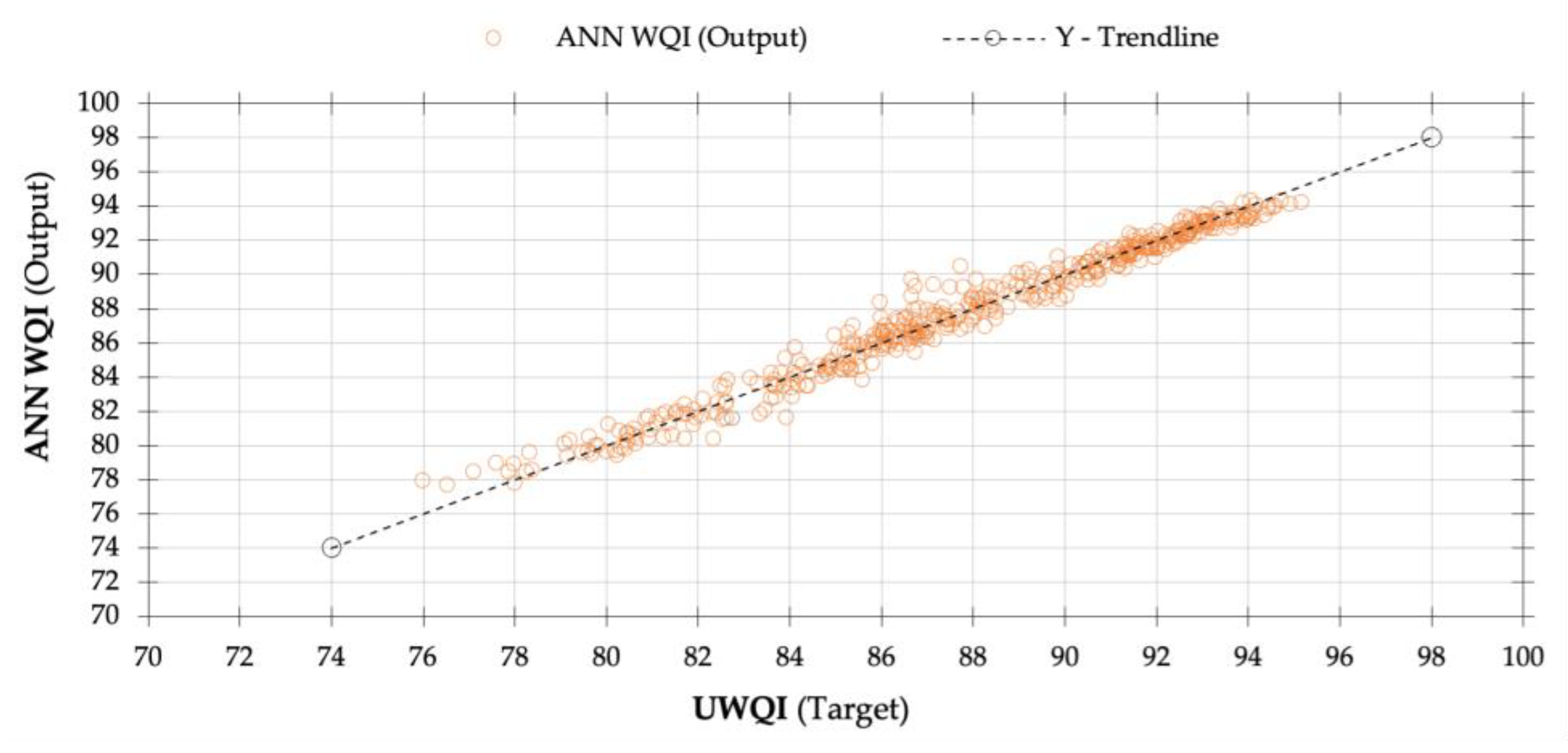
The artificial neural network model demonstrated a reasonably high degree of accuracy, recording an overall correlation coefficient (R) of 0.985 (p < 0.01) while having specific R-values of 0.987, 0.992, and 0.977 for training, testing, and validation, respectively. The correlation coefficient outlines the neural network’s estimation capacity, with ratings beyond 0.5 being acceptable and values close to 1.0 being the most desirable because they depict superior models [66]. Accordingly, the current study accomplished satisfactorily high R-values nearing 1.0, thus demonstrating exceptional performance levels and a well-balanced neural network. The coefficient of determination (R2) explains the goodness-of-fit and the performance statistic R2 corresponds with the Nash–Sutcliffe efficiency (NSE) [65], whereby the finest optimal neural model is defined using the most significant value of R2 varying between zero and one, where greater values nearing one are desirable [3,17,66,71,74]. Nonetheless, coefficient of determination values surpassing 0.5 are considered satisfactory and acceptable. The suggested neural network has an NSE/R2 value measuring 0.970, implying that the AI-based model captures approximately 97% of variations of the observed water quality records. The ANN model displayed an average target-to-output error rating of ±0.242, meaning that the proposed WQI model has sufficient predictive capabilities, offering output scores identical to the target UWQI, registering minimum and maximum WQI values of 75.995 and 94.420, respectively. Figure 7 and Figure 8 indicate the relationship between the target UWQI and ANN output WQI.
Furthermore, the study measured the root mean squared error (RMSE) and mean absolute error (MAE) statistics, having ratings of 0.693 and 0.521, respectively. RMSE and MAE are standard quantitative performance statistics that evaluate the model’s estimation abilities and the matrices extending from zero to infinite figures. These performance evaluators are negatively oriented numbers, meaning smaller values are more appropriate, indicating superior predictive models [66,71]. The AI-based WQI model registered a mean absolute percentage error (MAPE) of 0.600%, confirming the suggested neural network has high accuracy (see ratings in Table 9). MAPE describes the model’s accuracy as a percentage, where zero depicts an excellent fit. MAPE has no maximum limit, but estimation tools with MAPE ratings exceeding 50% are considered unreliable [66]. Considering these performance evaluators, the suggested ANN-based WQI model is robust and scientifically balanced.

3.3. Sensitivity Analysis

Sensitivity analysis (SA) effectively evaluates essential factors contributing to the output scores and assesses the interrelationship among parameters in multivariable datasets [15,90]. SA allows for proper apportion of the uncertainty in outputs to the variability of the input variables over their entire domain of interest. The analysis explains the input parameter that contributes the most toward specific output patterns.
Global sensitivity analysis involves different input factors being altered simultaneously, while sensitivity is evaluated over the full range of the input factors. The sensitivity analysis measures the influence of network inputs and their effect on the network output [91]. The approach best fits non-linear input-to-output relationships; even more significantly, the method is more feasible considering that the strategy allows the impact of all input variables to be examined simultaneously without challenges [15,91]. Global sensitivity techniques include the Monte Carlo-based regression-correlation indices, Fourier amplitude sensitivity test (FAST), and Sobol’s sensitivity estimates. Respectively, the current research applied the Fourier amplitude sensitivity test, and the FAST outcome shows that the suggested artificial neural network is computationally robust and technically stable.
Furthermore, the study conducted a pointwise sensitivity analysis to examine the local patterns and sensitivity at specific data points, thus explaining linkages between the focal points and neighbours [90]. To better understand the usefulness of pointwise analysis, the method assisted in outlining how water quality index scores are influenced by a particular input variable, either positively or negatively. Furthermore, the pointwise approach describes the parameters significantly influencing water quality indexing [90]. The reasoning is that considering the correlation between WQI values (y-variables) and water quality indicators (x1, x2, …, x3), sensitivity analysis demonstrates the variation rate of y-variables as xi fluctuates [90]. Each x-parameter is altered using an outlier factor to determine anomalous local patterns that cannot comply with the global pattern. Pointwise sensitivity analysis substantiated the soundness and analytical aptitude of the proposed ANN-based WQI model.

3.4. Assessing Spatial and Temporal Trends

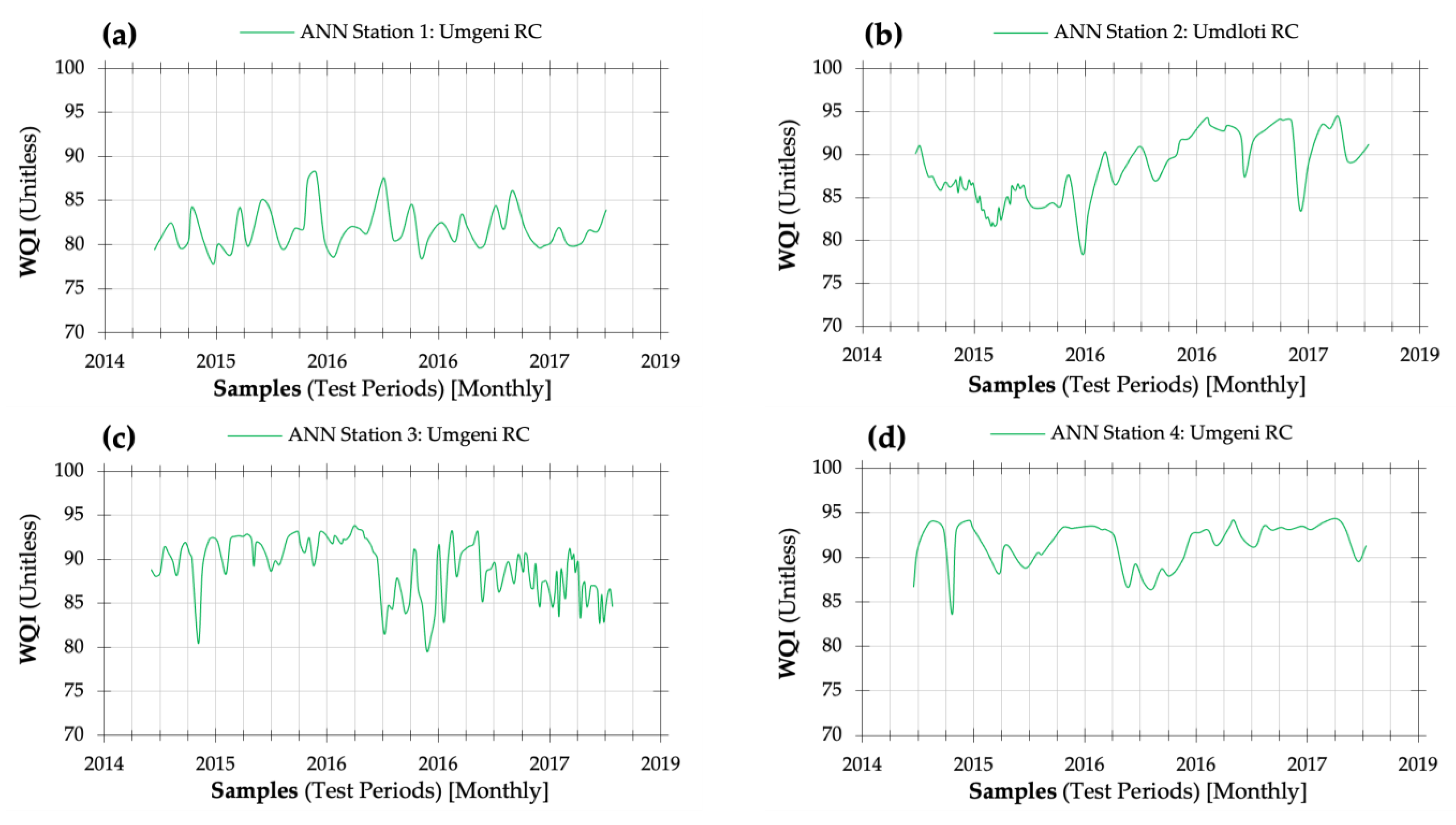
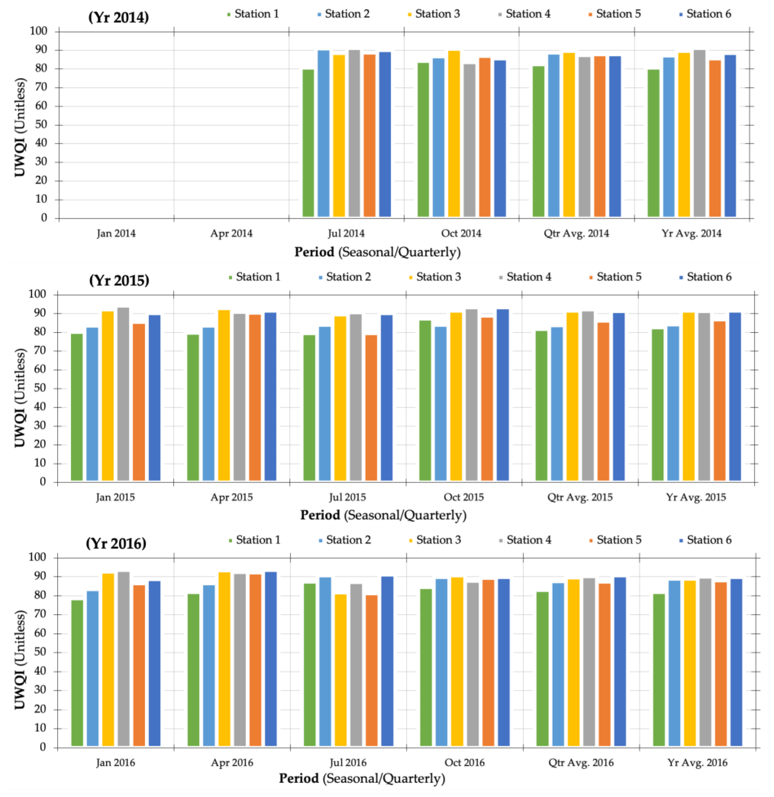
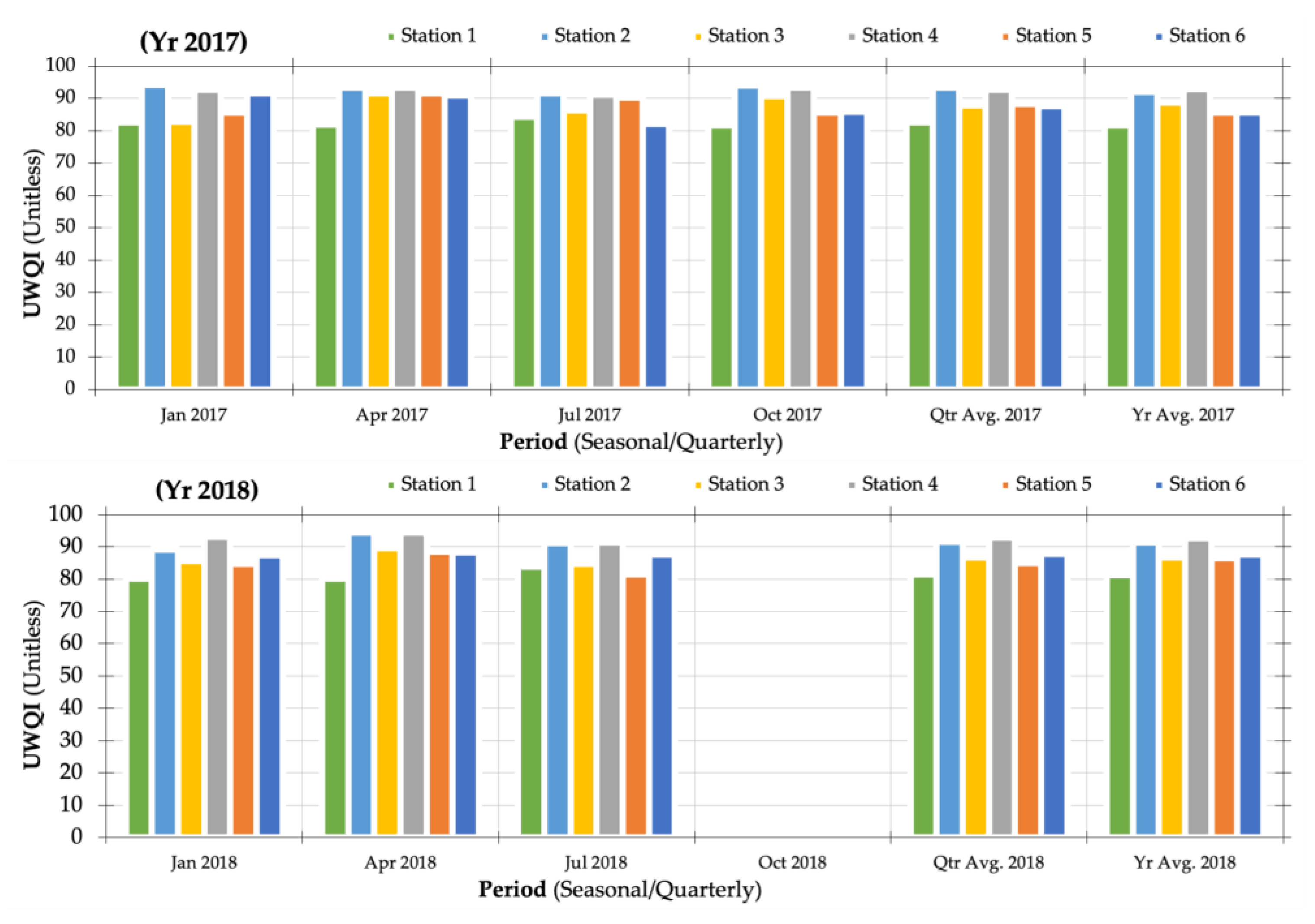
Four-year water quality records from Umgeni Water Board (UWB) were evaluated using the ANN WQI model to investigate spatial and temporal trends among the six monitoring stations (see Table 2). The spatiotemporal water quality patterns are documented in Figure 8, Figure 9 and Figure 10.
Using WQI outputs from the proposed ANN WQI model, the index results show that water quality within the four river basins can be categorised as Class 2 (acceptable). The drainage region has a minimal index value measuring 76.64 (Class 2), which corresponds to monitoring Station 3 for Inanda Dam within the Umgeni River basin. The lowest WQI rating is influenced by high concentration levels of Chl-a and NO3, having observed parameter values of 19.50 mg/ℓ and 1.31 mg/ℓ, respectively. Monitoring Station 4, situated at Midmar Dam within the Umgeni River basin, had the highest WQI value of 94.34 (Class 2) in April 2018 (Figure 9 and Figure 10).
Excessive levels of NO3 are observed during summertime, with anthropogenic activities being the possible source of pollution, primarily when considering the socioeconomic operations around the water quality monitoring locations. As a common and naturally forming ion, NO3 is perceived as the most notable contaminant influencing river systems. When viewed independently, nitrate is a low-toxicity compound; however, when transformed into nitrite (NO2), the parameter becomes progressively harmful to human health and aquatic life. Hence, routine water quality monitoring becomes imperative, thus continuously assessing water quality patterns over time and space is necessary to identify alarming trends. Like NO3, high turbidity levels are also evident during summertime due to various sources, including decomposition of organic matter, soil erosion, algal blooms, industrial effluent, wastewater, and reservoir drawdown flashing. When combined with NO3, turbidity contributes substantially towards the deterioration of water quality within the four river catchments. Chl-a concentration levels are impacted by eutrophication caused by soluble nutrients originating from phosphorus and nitrogen compounds. These enriching nutrients frequently emerge from human-based operations, including but not limited to fertiliser runoff and wastewater discharge.
Assessing water quality trends for different catchment areas supports the objective of developing water quality monitoring tools with widespread applications. The suggested ANN-based WQI model is significant because it can simulate water quality index values produced by the universal water quality index (UWQI) model (Figure 8). The similarity between the UWQI ratings and ANN model values is exceptional, with both having similar estimation patterns. Such predictive accuracy upholds the ability of the neural network to appraise the health of surface water resources, examine spatiotemporal water quality patterns, and identify alarming trends within the South African river catchments.

3.5. Index Categorisation Schema

The water quality index (WQI) ratings from the suggested artificial neural network (ANN) are categorised using a five-class classification schema. The ranking criterion follows an ascending scale identical to the ordinary percentage hierarchy. The mechanism better explains the index categorisation schema (water classification scale), specifically for non-technical people. Like the techniques applied by Abrahão et al. [92], Rubio-Arias et al. [93], Rabee et al. [94], and Sutadian et al. [95], appropriate mathematical functions with logical linguistic descriptors such as “less than”, “equal to”, and “greater than” are designated to each categorisation class. Table 10 and Figure 11 represent the index categorisation schema.
Under these conditions, the classification scale can accommodate every possible scenario and rank all index scores irrespective of the decimal value. More significantly, the proposed water classification scale helps close gaps identified in the literature and presents a progressive approach that will contribute considerably towards developing water quality indices (WQIs). Such academic and technical contributions indicate the model’s efficiency and contribute to the success of the research study.

4. Conclusions

Comparable with statistically developed models, neural networks are established using the target (dependent) variables; consequently, their estimation accuracy and reliability rely upon the performance levels of the parent model responsible for outputting the target variables. Without due diligence, challenges originating from the primary (founding) model might be carried forward and impact the latter (newer) model. In this case, index values generated by the universal water quality index (UWQI) and water quality records from Umgeni were applied to develop an interconnected neural network model. The dataset comprises 416 water quality samples with thirteen indicators observed monthly in six different monitoring locations for a period exceeding four years. The UWQI scores depict the target or dependent variables, and the Umgeni water quality parameters signify the explanatory or independent variables for developing the ANN.
The computational capabilities of artificial intelligence (AI) algorithms in appraising spatiotemporal water quality trends were investigated. The current study suggests a three-layer parallel-distributed feed-forward neural network model for monitoring long-term spatial and temporal water quality fluctuations within South African river systems. The ANN model demonstrated a comparatively high degree of accuracy, having an overall correlation coefficient (R) and coefficient of determination (R2) measuring 0.985 and 0.970, respectively. Furthermore, the R-values obtained are satisfactory, indicating higher predictive performance and a scientifically stable and well-defined neural network. The research findings suggest that artificial neural networks (ANNs) are robust and practical analytical tools for assessing surface water quality.
The results further exhibit the appropriateness of modelling ANNs as a powerful alternative to conventional and statistical modelling techniques, thereby satisfying the research hypothesis, which states that: “the ANN model should be more robust and scientifically stable, with better predictive performance than traditional WQI models”. Accordingly, the study encourages water resources professionals and scientists to consider neural networks to be an extensive and remarkably effective approach for assessing water quality patterns. Against this background, artificial neural networks are recommended for routine monitoring of surface water resources. Hopefully, the study will provide meaningful contributions and a valuable platform for applying artificial neural networks.

Author Contributions

Conceptualization, T.D.B. and M.K.; methodology, T.D.B.; software, T.D.B.; validation, T.D.B. and M.K.; formal analysis, T.D.B.; investigation, T.D.B.; resources, T.D.B. and M.K.; data curation, T.D.B.; writing—original draft preparation, T.D.B.; writing—review and editing, T.D.B. and M.K.; visualization, T.D.B.; supervision, M.K.; project administration, T.D.B.; funding acquisition, T.D.B. and M.K. All authors have read and agreed to the published version of the manuscript.

Funding

This research was funded by ZAKUMI Consulting Engineers (Pty) Ltd., grant number ST2017/BANDA/PhD-Eng/UKZN, and the study was supported by the University of KwaZulu-Natal.

Data Availability Statement

All data, models, and code generated or used during the study appear in the submitted article. Further data can be obtained in the Doctoral Thesis at https://researchspace.ukzn.ac.za/handle/10413/19877 (accessed 15 December 2021).

Acknowledgments

Our utmost gratitude is extended to the staff members of the Research Office of the University of KwaZulu-Natal for supporting this research publication.

Conflicts of Interest

The authors declare no conflicts of interest. The funders had no role in preparing this paper; in the collection, analysis, or interpretation of data; in the writing of the manuscript, or in the decision to publish the article.

References

  1. Nayak, J.G.; Patil, L.G.; Patki, V.K. Artificial neural network based water quality index (WQI) for river Godavari (India). Mater. Today Proc. 2023, 81, 212–220. [Google Scholar] [CrossRef]
  2. Pany, R.; Rath, A.; Swain, P.C. Water quality assessment for River Mahanadi of Odisha, India using statistical techniques and Artificial Neural Networks. J. Clean. Prod. 2023, 417, 137713. [Google Scholar] [CrossRef]
  3. Gazzaz, N.M.; Yusoff, M.K.; Aris, A.Z.; Juahir, H.; Ramli, M.F. Artificial neural network modeling of the water quality index for Kinta River (Malaysia) using water quality variables as predictors. Mar. Pollut. Bull. 2012, 64, 2409–2420. [Google Scholar] [CrossRef] [PubMed]
  4. García-Alba, J.; Bárcena, J.F.; Ugarteburu, C.; García, A. Artificial neural networks as emulators of process-based models to analyse bathing water quality in estuaries. Water Res. 2019, 150, 283–295. [Google Scholar] [CrossRef]
  5. Kulisz, M.; Kujawska, J. Application of artificial neural network (ANN) for water quality index (WQI) prediction for the river Warta, Poland. J. Phys. Conf. Ser. 2021, 2130, 012028. [Google Scholar] [CrossRef]
  6. Singh, K.P.; Basant, A.; Malik, A.; Jain, G. Artificial neural network modeling of the river water quality—A case study. Ecol. Model. 2009, 220, 888–895. [Google Scholar] [CrossRef]
  7. Khalil, B.; Ouarda, T.; St-Hilaire, A. Estimation of water quality characteristics at ungauged sites using artificial neural networks and canonical correlation analysis. J. Hydrol. 2011, 405, 277–287. [Google Scholar] [CrossRef]
  8. Kim, S.E.; Seo, I.W. Artificial neural network ensemble modeling with conjunctive data clustering for water quality prediction in rivers. J. Hydro-Environ. Res. 2015, 9, 325–339. [Google Scholar] [CrossRef]
  9. Sarkar, A.; Pandey, P. River water quality modelling using artificial neural network technique. Aquat. Procedia 2015, 4, 1070–1077. [Google Scholar] [CrossRef]
  10. Salari, M.; Salami Shahid, E.; Afzali, S.H.; Ehteshami, M.; Conti, G.O.; Derakhshan, Z.; Sheibani, S.N. Quality assessment and artificial neural networks modeling for characterization of chemical and physical parameters of potable water. Food Chem. Toxicol. 2018, 118, 212–219. [Google Scholar] [CrossRef]
  11. Ramasubramanian, K.; Singh, A. Machine learning theory and practice. In Machine Learning Using R: With Time Series and Industry-Based Use Cases in R; Ramasubramanian, K., Singh, A., Eds.; Apress: Berkeley, CA, USA, 2019; pp. 253–481. [Google Scholar] [CrossRef]
  12. De Sousa, W.G.; de Melo, E.R.P.; Bermejo, P.H.D.S.; Farias, R.A.S.; Gomes, A.O. How and where is artificial intelligence in the public sector going? A literature review and research agenda. Gov. Inf. Q. 2019, 36, 101392. [Google Scholar] [CrossRef]
  13. Li, D.; Liu, S. Chapter 4—Water quality evaluation. In Water Quality Monitoring and Management; Li, D., Liu, S., Eds.; Academic Press: Cambridge, MA, USA, 2019; pp. 113–159. [Google Scholar] [CrossRef]
  14. Ibrahim, A.; Ismail, A.; Juahir, H.; Iliyasu, A.B.; Wailare, B.T.; Mukhtar, M.; Aminu, H. Water quality modelling using principal component analysis and artificial neural network. Mar. Pollut. Bull. 2023, 187, 114493. [Google Scholar] [CrossRef] [PubMed]
  15. Huo, S.; He, Z.; Su, J.; Xi, B.; Zhu, C. Using artificial neural Network models for eutrophication prediction. Procedia Environ. Sci. 2013, 18, 310–316. [Google Scholar] [CrossRef]
  16. Seo, I.w.; Yun, S.H.; Choi, S.Y. Forecasting water quality parameters by ANN model using pre-processing technique at the downstream of Cheongpyeong Dam. Procedia Eng. 2016, 154, 1110–1115. [Google Scholar] [CrossRef]
  17. Qaderi, F.; Babanezhad, E. Prediction of the groundwater remediation costs for drinking use based on quality of water resource, using artificial neural network. J. Clean. Prod. 2017, 161, 840–849. [Google Scholar] [CrossRef]
  18. Bansal, S.; Ganesan, G. Advanced evaluation methodology for water quality assessment using artificial neural network approach. Water Resour. Manag. 2019, 33, 3127–3141. [Google Scholar] [CrossRef]
  19. Kadam, A.K.; Wagh, V.M.; Muley, A.A.; Umrikar, B.N.; Sankhua, R.N. Prediction of water quality index using artificial neural network and multiple linear regression modelling approach in Shivganga River basin, India. Model. Earth Syst. Environ. 2019, 5, 951–962. [Google Scholar] [CrossRef]
  20. Isiyaka, H.A.; Mustapha, A.; Juahir, H.; Phil-Eze, P. Water quality modelling using artificial neural network and multivariate statistical techniques. Model. Earth Syst. Environ. 2019, 5, 583–593. [Google Scholar] [CrossRef]
  21. Soro, M.-P.; Yao, K.M.; Kouassi, N.G.L.B.; Ouattara, A.A.; Diaco, T. Modeling the spatio-temporal evolution of chlorophyll-a in three tropical rivers Comoé, Bandama, and Bia Rivers (Côte d’Ivoire) by artificial neural network. Wetlands 2020, 40, 939–956. [Google Scholar] [CrossRef]
  22. Fartas, F.; Remini, B.; Sekiou, F.; Marouf, N. The use of PCA and ANN to improve evaluation of the WQIclassic, development of a new index, and prediction of WQI, Coastel Constantinois, northern coast of eastern Algeria. Water Supply 2022, 22, 8727–8749. [Google Scholar] [CrossRef]
  23. Elkiran, G.; Nourani, V.; Abba, S.I. Multi-step ahead modelling of river water quality parameters using ensemble artificial intelligence-based approach. J. Hydrol. 2019, 577, 123962. [Google Scholar] [CrossRef]
  24. Tiyasha; Tung, T.M.; Yaseen, Z.M. A survey on river water quality modelling using artificial intelligence models: 2000–2020. J. Hydrol. 2020, 585, 124670. [Google Scholar] [CrossRef]
  25. Banda, T.D.; Kumarasamy, M. Application of multivariate statistical analysis in the development of a surrogate water quality index (WQI) for South African watersheds. Water 2020, 12, 1584. [Google Scholar] [CrossRef]
  26. Banda, T.D. Development of a Universal Water Quality Index and Water Quality Variability Model for South African River Catchments. Ph.D. Thesis, University of KwaZulu-Natal, Durban, South Africa, 2020. [Google Scholar]
  27. Banda, T.D.; Kumarasamy, M. Development of a universal water quality index (UWQI) for South African river catchments. Water 2020, 12, 1534. [Google Scholar] [CrossRef]
  28. Horton, R.K. An index-number system for rating water quality. J. Water Pollut. Control. Fed. 1965, 37, 300–306. [Google Scholar]
  29. Brown, R.M.; McClelland, N.I.; Deininger, R.A.; Tozer, R.G. A water quality index—Do we dare? Water Sew. Work. 1970, 117, 339–343. [Google Scholar]
  30. Linstone, H.A.; Turoff, M. The Delphi Method: Techniques and Applications; Addison-Wesley Reading: Boston, MA, USA, 1975; Volume 29. [Google Scholar]
  31. Woudenberg, F. An evaluation of Delphi. Technol. Forecast. Soc. Chang. 1991, 40, 131–150. [Google Scholar] [CrossRef]
  32. Nagels, J.; Davies-Colley, R.; Smith, D. A water quality index for contact recreation in New Zealand. Water Sci. Technol. 2001, 43, 285–292. [Google Scholar] [CrossRef] [PubMed]
  33. Linstone, H.A.; Turoff, M. The Delphi Method: Techniques and Applications; Addison-Wesley Publishing Co.: Newark, NJ, USA, 2002; Volume 18. [Google Scholar]
  34. Kumar, D.; Alappat, B.J. NSF-Water quality index: Does it represent the experts’ opinion? Pract. Period. Hazard. Toxic Radioact. Waste Manag. 2009, 13, 75–79. [Google Scholar] [CrossRef]
  35. Almeida, C.; González, S.O.; Mallea, M.; González, P. A recreational water quality index using chemical, physical and microbiological parameters. Environ. Sci. Pollut. Res. 2012, 19, 3400–3411. [Google Scholar] [CrossRef]
  36. Namugize, J.N.; Jewitt, G.; Graham, M. Effects of land use and land cover changes on water quality in the uMngeni river catchment, South Africa. Phys. Chem. Earth Parts A/B/C 2018, 105, 247–264. [Google Scholar] [CrossRef]
  37. Shoko, C. The Effect of Spatial Resolution in Remote Sensing Estimates of Total Evaporation in the uMgeni Catchment. Master’s Thesis, University of KwaZulu-Natal, Pietermaritzburg, South Africa, 2014. [Google Scholar]
  38. Hughes, C.; de Winnaar, G.; Schulze, R.; Mander, M.; Jewitt, G. Mapping of water-related ecosystem services in the uMngeni catchment using a daily time-step hydrological model for prioritisation of ecological infrastructure investment–Part 1: Context and modelling approach. Water SA 2018, 44, 577–589. [Google Scholar] [PubMed]
  39. Umgeni Water. Infrastructure Master Plan 2019/2020-2049/2050, Volume 2: Mgeni System; Umgeni Water: Pietermaritzburg, South Africa, 2019; p. 185. [Google Scholar]
  40. Umgeni Water. Infrastructure Master Plan 2019/2020-2049/2050, Volume 3: uMkhomazi System; Umgeni Water: Pietermaritzburg, South Africa, 2019; p. 35. [Google Scholar]
  41. Department of Water and Environmental Affairs (Ed.) Proposed new nine (9) water management areas of South Africa. In Government Gazette No. 35517, Notice No. 547; Department of Water and Environmental Affairs: Pretoria, South Africa, 2012; Volume 565, p. 72. [Google Scholar]
  42. Chiluwe, Q.W. Assessing the Role of Property Rights in Managing Water Demand: The Case of uMgeni River Catchment. Master’s Thesis, Monash South Africa, Roodepoort, South Africa, 2014. [Google Scholar]
  43. Warburton, M.L.; Schulze, R.E.; Jewitt, G.P.W. Hydrological impacts of land use change in three diverse South African catchments. J. Hydrol. 2012, 414–415, 118–135. [Google Scholar] [CrossRef]
  44. Rangeti, I. Determinants of Key Drivers for Potable Water Treatment Cost in uMngeni Basin. Master’s Thesis, Durban University of Technology, Durban, South Africa, 2015. [Google Scholar]
  45. Olaniran, A.O.; Naicker, K.; Pillay, B. Assessment of physico-chemical qualities and heavy metal concentrations of Umgeni and Umdloti Rivers in Durban, South Africa. Environ. Monit. Assess. 2014, 186, 2629–2639. [Google Scholar] [CrossRef] [PubMed]
  46. Gakuba, E.; Moodley, B.; Ndungu, P.; Birungi, G. Occurrence and significance of polychlorinated biphenyls in water, sediment pore water and surface sediments of Umgeni River, KwaZulu-Natal, South Africa. Environ. Monit. Assess. 2015, 187, 568. [Google Scholar] [CrossRef] [PubMed]
  47. Namugize, J.N.; Jewitt, G.P.W. Sensitivity analysis for water quality monitoring frequency in the application of a water quality index for the uMngeni River and its tributaries, KwaZulu-Natal, South Africa. Water SA 2018, 44, 516–527. [Google Scholar] [CrossRef]
  48. Umgeni Water. Infrastructure Paster Plan 2019/2020-2049/2050, Volume 5: North Coast System; Umgeni Water: Pietermaritzburg, South Africa, 2019; p. 116. [Google Scholar]
  49. Govender, S. An Investigation of the Natural and Human Induced Impacts on the Umdloti Catchment. Master’s Thesis, University of KwaZulu-Natal, Durban, South Africa, 2009. [Google Scholar]
  50. Umgeni Water. Infrastructure Master Plan 2019/2020-2049/2050, Volume 4: South Coast System; Umgeni Water: Pietermaritzburg, South Africa, 2019; p. 116. [Google Scholar]
  51. Mwelase, L.T. Non-Revenue Water: Most Suitable Business Model for Water Services Authorities in South Africa: Ugu District Municipality. Master’s Thesis, Durban University of Technology, Durban, South Africa, 2016. [Google Scholar]
  52. Luzati, S.; Jaupaj, O. Assessment of water quality index of Durresi-Kavaja Basin, Albania. J. Int. Environ. Appl. Sci. 2016, 11, 277–284. [Google Scholar]
  53. Wanda, E.M.; Mamba, B.B.; Msagati, T.A. Determination of the water quality index ratings of water in the Mpumalanga and North West provinces, South Africa. Phys. Chem. Earth 2016, 92, 70–78. [Google Scholar] [CrossRef]
  54. Guettaf, M.; Maoui, A.; Ihdene, Z. Assessment of water quality: A case study of the Seybouse River (North East of Algeria). Appl. Water Sci. 2017, 7, 295–307. [Google Scholar] [CrossRef]
  55. Paun, I.; Cruceru, L.V.; Chiriac, L.F.; Niculescu, M.; Vasile, G.G.; Marin, N.M. Water Quality Indices-methods for evaluating the quality of drinking water. In Proceedings of the 19th INCD ECOIND International Symposium-SIMI 2016, “The Environment and the Industry”, Bucharest, Romania, 13–14 October 2016; pp. 395–402. [Google Scholar]
  56. Banda, T.D. Developing an Equitable Raw Water Pricing Model: The Vaal Case Study. Master’s Thesis, Tshwane University of Technology, Pretoria, South Africa, 2015. [Google Scholar]
  57. Banda, T.D.; Kumarasamy, M.V. Development of water quality indices (WQIs): A review. Pol. J. Environ. Stud. 2020, 29, 2011–2021. [Google Scholar] [CrossRef]
  58. DWAF. South African Water Quality Guidelines: Volume 1: Domestic Water Use; Department of Water Affairs and Forestry: Pretoria, South Africa, 1996; p. 190. [Google Scholar]
  59. DWAF. South African Water Quality Guidelines: Volume 3: Industrial Use; Department of Water Affairs and Forestry: Pretoria, South Africa, 1996. [Google Scholar]
  60. DWAF. South African Water Quality Guidelines: Volume 7: Aquatic Ecosystems; Department of Water Affairs and Forestry: Pretoria, South Africa, 1996. [Google Scholar]
  61. TIBCO Software Inc. TIBCO Statistica Automated Neural Networks (SANN) Software, 13.6.0; TIBCO Software Inc.: Palo Alto, CA, USA; Arlington, TX, USA, 2020.
  62. Kim, H.G.; Hong, S.; Jeong, K.-S.; Kim, D.-K.; Joo, G.-J. Determination of sensitive variables regardless of hydrological alteration in artificial neural network model of chlorophyll a: Case study of Nakdong River. Ecol. Model. 2019, 398, 67–76. [Google Scholar] [CrossRef]
  63. Fletcher, D.; Goss, E. Forecasting with neural networks: An application using bankruptcy data. Inf. Manag. 1993, 24, 159–167. [Google Scholar] [CrossRef]
  64. Alyuda Research Inc. NeuroIntelligence Software, 2.1; Alyuda Research Inc.: Los Altos, CA, USA, 2003.
  65. Palani, S.; Liong, S.-Y.; Tkalich, P. An ANN application for water quality forecasting. Mar. Pollut. Bull. 2008, 56, 1586–1597. [Google Scholar] [CrossRef] [PubMed]
  66. Rajaee, T.; Khani, S.; Ravansalar, M. Artificial intelligence-based single and hybrid models for prediction of water quality in rivers: A review. Chemom. Intell. Lab. Syst. 2020, 200, 103978. [Google Scholar] [CrossRef]
  67. Mitrović, T.; Antanasijević, D.; Lazović, S.; Perić-Grujić, A.; Ristić, M. Virtual water quality monitoring at inactive monitoring sites using Monte Carlo optimized artificial neural networks: A case study of Danube River (Serbia). Sci. Total Environ. 2019, 654, 1000–1009. [Google Scholar] [CrossRef] [PubMed]
  68. Lucio, P.S.; Conde, F.C.; Cavalcanti, I.F.A.; Serrano, A.I.; Ramos, A.M.; Cardoso, A.O. Spatiotemporal monthly rainfall reconstruction via artificial neural network? Case study: South of Brazil. Adv. Geosci. 2007, 10, 67–76. [Google Scholar] [CrossRef]
  69. Shanthi, D.; Sahoo, G.; Saravanan, N. Comparison of neural network training algorithms for the prediction of the patient’s post-operative recovery area. J. Converg. Inf. Technol. 2009, 4, 24–32. [Google Scholar] [CrossRef]
  70. Banerjee, P.; Singh, V.S.; Chatttopadhyay, K.; Chandra, P.C.; Singh, B. Artificial neural network model as a potential alternative for groundwater salinity forecasting. J. Hydrol. 2011, 398, 212–220. [Google Scholar] [CrossRef]
  71. Safavi, H.R.; Malek Ahmadi, K. Prediction and assessment of drought effects on surface water quality using artificial neural networks: Case study of Zayandehrud River, Iran. J. Environ. Health Sci. Eng. 2015, 13, 68. [Google Scholar] [CrossRef]
  72. Gebler, D.; Wiegleb, G.; Szoszkiewicz, K. Integrating river hydromorphology and water quality into ecological status modelling by artificial neural networks. Water Res. 2018, 139, 395–405. [Google Scholar] [CrossRef]
  73. Ahamad, K.U.; Raj, P.; Barbhuiya, N.H.; Deep, A. Surface water quality modeling by regression analysis and artificial neural network. In Advances in Waste Management; Springer: Singapore, 2019; pp. 215–230. [Google Scholar] [CrossRef]
  74. Charulatha, G.; Srinivasalu, S.; Uma Maheswari, O.; Venugopal, T.; Giridharan, L. Evaluation of ground water quality contaminants using linear regression and artificial neural network models. Arab. J. Geosci. 2017, 10, 128. [Google Scholar] [CrossRef]
  75. Ye, Z.; Yang, J.; Zhong, N.; Tu, X.; Jia, J.; Wang, J. Tackling environmental challenges in pollution controls using artificial intelligence: A review. Sci. Total Environ. 2020, 699, 134279. [Google Scholar] [CrossRef] [PubMed]
  76. Aalipour, M.; Šťastný, B.; Horký, F.; Jabbarian Amiri, B. Scaling an artificial neural network-based water quality index model from small to large catchments. Water 2022, 14, 920. [Google Scholar] [CrossRef]
  77. Yilma, M.; Kiflie, Z.; Windsperger, A.; Gessese, N. Application of artificial neural network in water quality index prediction: A case study in Little Akaki River, Addis Ababa, Ethiopia. Model. Earth Syst. Environ. 2018, 4, 175–187. [Google Scholar] [CrossRef]
  78. Azimi, S.; Azhdary Moghaddam, M.; Hashemi Monfared, S.A. Prediction of annual drinking water quality reduction based on Groundwater Resource Index using the artificial neural network and fuzzy clustering. J. Contam. Hydrol. 2019, 220, 6–17. [Google Scholar] [CrossRef] [PubMed]
  79. Lu, F.; Zhang, H.; Liu, W. Development and application of a GIS-based artificial neural network system for water quality prediction: A case study at the Lake Champlain area. J. Oceanol. Limnol. 2019, 38, 1835–1845. [Google Scholar] [CrossRef]
  80. Vijay, S.; Kamaraj, K. Prediction of water quality index in drinking water distribution system using activation functions based ANN. Water Resour. Manag. 2021, 35, 535–553. [Google Scholar] [CrossRef]
  81. Cordoba, G.A.C.; Tuhovčák, L.; Tauš, M. Using artificial neural network models to assess water quality in water distribution networks. Procedia Eng. 2014, 70, 399–408. [Google Scholar] [CrossRef]
  82. Haldorai, A.; Ramu, A.; Murugan, S. Artificial intelligence and machine learning for future urban development. In Computing and Communication Systems in Urban Development: A Detailed Perspective; Haldorai, A., Ramu, A., Murugan, S., Eds.; Springer International Publishing: Cham, Switzerland, 2019; pp. 91–113. [Google Scholar] [CrossRef]
  83. Lischeid, G. Investigating short-term dynamics and long-term trends of SO4 in the runoff of a forested catchment using artificial neural networks. J. Hydrol. 2001, 243, 31–42. [Google Scholar] [CrossRef]
  84. Mas, D.M.L.; Ahlfeld, D.P. Comparing artificial neural networks and regression models for predicting faecal coliform concentrations. Hydrol. Sci. J. 2007, 52, 713–731. [Google Scholar] [CrossRef]
  85. Olszewski, T.; Ryniecki, A.; Boniecki, P. Neural network development for automatic identification of the endpoint of drying barley in bulk. J. Res. Appl. Agric. Eng. 2008, 53, 26–31. [Google Scholar]
  86. May, D.B.; Sivakumar, M. Prediction of urban stormwater quality using artificial neural networks. Environ. Model. Softw. 2009, 24, 296–302. [Google Scholar] [CrossRef]
  87. Amiri, B.; Nakane, K. Comparative prediction of stream water total nitrogen from land cover using artificial neural network and multiple linear regression. Pol. J. Environ. Stud. 2009, 18, 151–160. [Google Scholar]
  88. Oliveira Souza da Costa, A.; Ferreira Silva, P.; Godoy Sabará, M.; Ferreira da Costa, E. Use of neural networks for monitoring surface water quality changes in a neotropical urban stream. Environ. Monit. Assess. 2009, 155, 527–538. [Google Scholar] [CrossRef] [PubMed]
  89. Kulisz, M.; Kujawska, J.; Przysucha, B.; Cel, W. Forecasting water quality index in groundwater using artificial neural network. Energies 2021, 14, 5875. [Google Scholar] [CrossRef]
  90. Guo, Z.; Ward, M.; Rundensteiner, E.; Ruiz, C. Pointwise local pattern exploration for sensitivity analysis. In Proceedings of the 2011 IEEE Conference on Visual Analytics Science and Technology (VAST), Providence, RI, USA, 23–28 October 2011; pp. 131–140. [Google Scholar]
  91. Zhou, X.; Lin, H.; Lin, H. Global sensitivity analysis. In Encyclopedia of GIS; Shekhar, S., Xiong, H., Eds.; Springer: Boston, MA, USA, 2008; pp. 408–409. [Google Scholar] [CrossRef]
  92. Abrahão, R.; Carvalho, M.; da Silva, W., Jr.; Machado, T.; Gadelha, C.; Hernandez, M. Use of index analysis to evaluate the water quality of a stream receiving industrial effluents. Water SA 2007, 33, 459–466. [Google Scholar] [CrossRef]
  93. Rubio-Arias, H.; Contreras-Caraveo, M.; Quintana, R.M.; Saucedo-Teran, R.A.; Pinales-Munguia, A. An overall water quality index (WQI) for a man-made aquatic reservoir in Mexico. Int. J. Environ. Res. Public Health 2012, 9, 1687–1698. [Google Scholar] [CrossRef]
  94. Rabee, A.M.; Al-Fatlawy, Y.F.; Nameer, M. Using pollution load index (PLI) and geoaccumulation index (I-Geo) for the assessment of heavy metals pollution in Tigris river sediment in Baghdad Region. Al-Nahrain J. Sci. 2011, 14, 108–114. [Google Scholar]
  95. Sutadian, A.D.; Muttil, N.; Yilmaz, A.G.; Perera, B.J.C. Development of a water quality index for rivers in West Java Province, Indonesia. Ecol. Indic. 2018, 85, 966–982. [Google Scholar] [CrossRef]
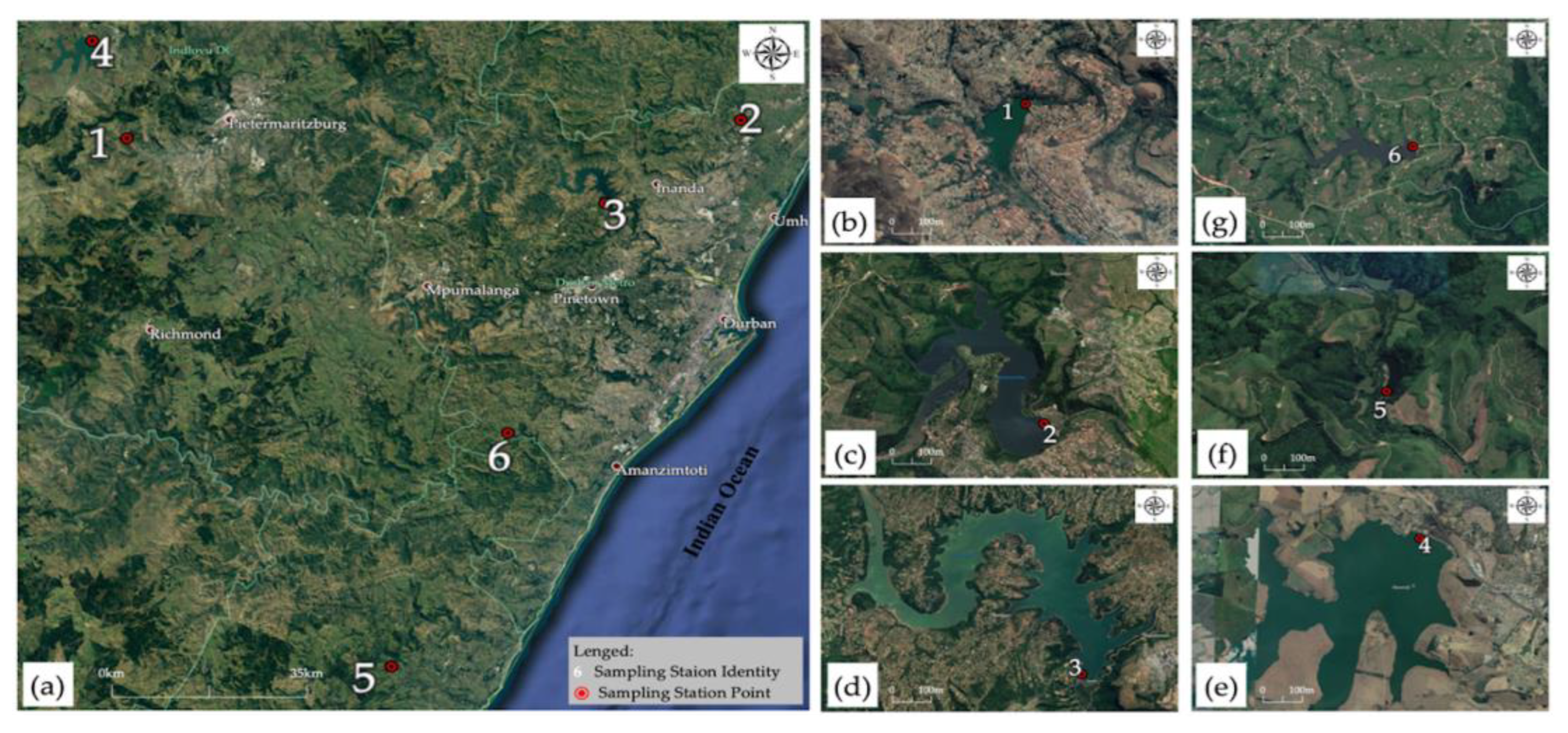
Figure 1. Locality map for water quality monitoring points: (a) six sampling stations, (b) Henley Dam, (c) Hazelmere Dam, (d) Inanda Dam, (e) Midmar Dam, (f) Umzinto Dam, and (g) Nungwane Dam. The location coordinates in Figure 1 are from UWB (Table 2), and the underlying maps originated from Google Earth. Notes: Monitoring Stations 1 to 6 represent Henley Dam (DHL003), Hazelmere Dam (DHM003), Inanda Dam (DIN003), Midmar Dam (DMM003), Umzinto Dam (DMZ009), and Nungwane Dam (DNW003), respectively. Source: Banda and Kumarasamy [25,27].
Water 16 01485 g001
Figure 2. The Water Quality Index Score Counts for the UWQI. Source: The universal water quality index (UWQI) results were extracted from Banda and Kumarasamy [27]. Plot diagram developed using TIBCO Software Inc. [61] from Palo Alto, California, USA.
Water 16 01485 g002
Figure 3. The logistic-sigmoidal activation function blueprint. Source: Diagram developed using Equation (4) as published by García-Alba et al. [4], Huo et al. [15], Palani et al. [65].
Water 16 01485 g003
Figure 4. A diagrammatic illustration of the feed-forward and error-backpropagation cycles for ANN-based models. Source: Kim and Seo [8], Banda [26].
Water 16 01485 g004
Figure 5. A schematic representation of the neuro-node operating cycle and feed-forward sequencing. Source: Banda [26].
Water 16 01485 g005
Figure 6. A block diagram illustrating the three-layer feed-forward artificial neural network. The ANN model features thirteen neurons within the input layer, five neuro-nodes in the hidden or “zero” layer, one output neuron, and seventy channel links connected left to right. The following publications discuss the adopted fundamental framework for developing ANN models: Nayak et al. [1], García-Alba et al. [4], Singh et al. [6], Sarkar and Pandey [9], Huo et al. [15], Seo et al. [16], Kim et al. [62], Yilma et al. [77], Cordoba et al. [81], Haldorai et al. [82].
Water 16 01485 g006
Figure 7. A scatter plot displaying ANN-based model validation results and demonstrating the relationship between the target UWQI scores and the equivalent ANN model estimations. The plot diagram indicates that the suggested ANN model achieved a sensible approximation throughout the spectrum of the UWQI scores. The overall agreement between the measured and simulated WQI ratings is satisfactory, having the following statistics: R of 0.985, p < 0.01; R2 of 97%; NSE of 0.970, RMSE of 0.692, MAPE of 0.600%, and n equal to 416. Source: Artificial neural network (ANN) model results generated using TIBCO Software Inc. [61].
Water 16 01485 g007
Figure 8. Comparing the universal water index scores (target UWQI) and artificial neural network WQI values (ANN output) including prediction error margins. Source: Artificial neural network (ANN) model results generated using TIBCO Software Inc. [61].
Water 16 01485 g008
Figure 9. Spatiotemporal water quality trends outlined using Umgeni data (2014 to 2018) and ANN WQI scores (a) Umgeni Catchment: Henley Dam, (b) Umdloti Catchment: Hazelmere Dam, (c) Umgeni Catchment: Inanda Dam, (d) Umgeni Catchment: Midmar Dam, (e) Umzinto/Umuziwezinto Catchment: Umzinto Dam, and (f) Nungwane Catchment: Nungwane Dam. Source: Artificial neural network (ANN) model results generated using TIBCO Software Inc. [61].
Water 16 01485 g009aWater 16 01485 g009b
Figure 10. Four-year seasonal water quality variability for Umgeni water quality records (June 2014 to July 2018). Source: Artificial neural network (ANN) model results generated using TIBCO Software Inc. [61].
Water 16 01485 g010aWater 16 01485 g010b
Figure 11. Index categorisation schema containing classification sub-schema and action blocks based on logical linguistic descriptors, where Class 1 index scores (excellent) are only attainable when all water quality indicators are within permissible limits virtually all the time. The water quality classification system follows the “green-yellow-red” colour gradient, consistent with applicable water quality categories ranging from good water quality (Class 1) to very bad water quality (Class 5). Source: Banda and Kumarasamy [25,27]; a redraft of the index categorisation schema proposed by Banda [56].
Water 16 01485 g011
Table 1. Descriptive statistics for measured monthly water quality records accessed from UWB.
Variables aStatistical Summary of Water Quality Data
MinimumMaximumAverageStandard Deviation
1NH30.0400.9900.1070.091
2Ca1.00030.5009.4576.078
3Cl1.82079.00026.84313.765
4Chl-a0.14092.2204.9999.374
5EC6.84048.00020.7089.840
6F0.1000.5400.1400.048
7CaCO36.620128.46047.7529.499
8Mg1.00014.6005.8572.535
9Mn0.0101.2100.0510.172
10NO30.0509.5800.5900.984
11pH0.0009.1007.7660.529
12SO40.16024.2008.6965.980
13Turb0.600367.00014.15729.638
Notes: Source: Umgeni Water Board (2014 to 2018). a Water quality variable measured in mg/ℓ, except for chlorophyll-a (µg/ℓ), electrical conductivity (µS/m), pondus Hydrogenium (unitless), and turbidity (NTU). Although the information from Umgeni contains more water quality parameters, Table 1 displays only the thirteen water quality indicators examined in the current research. Water quality variables are listed in alphabetic order rather than the order of importance.
Table 2. Water quality monitoring stations considered for this study.
Sampling StationLocation Coordinates in Degrees, Minutes, and Seconds (DMS) *
LatitudeLongitude
1Henley DamS 29°37′25.734″E 30°14′49.754″
2Hazelmere DamS 29°35′53.722″E 31°02′32.121″
3Inanda Dam 0.3 kmS 29°42′27.403″E 30°52′03.352″
4Midmar DamS 29°29′47.332″E 30°12′05.655″
5Umzinto DamS 30°18′40.676″E 30°35′34.580″
6Nungwane DamS 30°00′24.473″E 30°44′36.150″
Notes: Source: Umgeni Water Board (UWB) [25,27]. * The coordinates are based on the World Geodetic System 84. Even though the UWB has additional water quality monitoring locations, Table 2 and Figure 1 represent data from six water quality observation points selected for this research.
Table 3. UWQI input variables and applicable weighting coefficients.
Water Quality VariableUnitsWeighting Coefficients
Impact (bi)Weight (wi)
1Ammoniamg/ℓ3.93580.1035
2Calciummg/ℓ2.76120.0726
3Chloridemg/ℓ2.81960.0742
4Chlorophyll-aµg/ℓ1.36110.0358
5Electrical ConductivityµS/m2.63050.0692
6Fluoridemg/ℓ3.60590.0949
7Hardnessmg/ℓ2.23290.0587
8Magnesiummg/ℓ2.70000.0710
9Manganesemg/ℓ3.46090.0910
10Nitratemg/ℓ3.45600.0909
11pondus HydrogeniumUnitless3.46410.0911
12Sulphatemg/ℓ2.94390.0774
13TurbidityNTU2.64460.0696
Totals38.01671.0000
Notes: Source: Banda and Kumarasamy [25,27]. The summation of weighting coefficients totals one whole number, and water quality variables are documented alphabetically. Based on the universal water quality index (UWQI) weighted coefficients, the study achieved the following significance order: NH3 > F > pH > Mn > NO3 > SO4 > Cl > Ca > Mg > Turb > EC > CaCO3 > Chl-a.
Table 4. The sub-index equations established for the universal water quality index (UWQI) model.
VariableSub-Index FunctionsVariableSub-Index Functions
RangeSub-Index EquationRule SetRangeSub-Index EquationRule Set
1NH3 x a     1.4 SI a = 56.627 x a + 97.609 f(1) Otherwise SI g = 0 f(32)
1.4   <   x a 1.5 SI a   = 140 x a + 216 f(2)8Mg x h     30 SI h = 0.1667 x h + 100 f(33)
1.5   <   x a 2.0 SI a = 12 x a + 24 f(3) 30   <   x h 40 SI h = 2.0 x h + 155 f(34)
Otherwise SI a = 0 f(4) 40   <   x h     50 SI h = 5.0 x h + 275 f(35)
2Ca x b     46.70 SI b = 1.0707 x b + 100 f(5) 50   <   x h     90 SI h = 0.625 x h + 56.25 f(36)
46.70   <   x b     60 SI b = 2.0301 x b + 144.8 f(6) Otherwise SI h = 0 f(37)
60   <   x b     90 SI b = 0.7667 x b + 69 f(7)9Mn x i     0.05 SI i = 100 f(38)
Otherwise SI b = 0 f(8) 0.05   <   x i     0.30 SI i = 40 x i + 92 f(39)
3Cl x c     50 SI c = 100 f(9) 0.30   <   x i     0.53 SI i = 130.43 x i + 119.13 f(40)
50   <   x c     150 SI c = 0.4 x c + 110 f(10) 0.53   <   x i     1.53 SI i = 50 x i + 76.50 f(41)
150   <   x c     500 SI c = 0.1286 x c + 69.286 f(11) Otherwise SI i = 0 f(42)
500   <   x c     600 SI c = 5 f(12)10NO3 x j     0.1 SI j = 150 x j + 100 f(43)
Otherwise SI c = 0 f(13) 0.1   <   x j     0.5 SI j = 37.5 x j + 88.75 f(44)
4Chl-a x d     1 SI d = 100 f(14) 0.5   <   x j     1.0 SI j = 100 x j + 120 f(45)
1   <   x d     10 SI d = 3.3333 x d + 93.333 f(15) 1.0   <   x j     2.0 SI j = 20 x j + 40 f(46)
10   <   x d     20 SI d = 5 x d + 110 f(16) Otherwise SI j = 0 f(47)
20   <   x d     28 SI d = 1.25 x d + 35 f(17)11pH x k     4 SI k = 0 f(48)
Otherwise SI d = 0 f(18) 4   <   x k     7 SI k = 26.667 x k   86.667 f(49)
5EC x e     70 SI e = 100 f(19) 7   <   x k     8 SI k = 100 f(50)
70   <   x e     150 SI e = 0.125 x e + 98.75 f(20) 8   <   x k     11 SI k = 26.667 x k + 313.33 f(51)
150   <   x e     450 SI e = 0.2333 x e + 115 f(21) Otherwise SI k = 0 f(52)
Otherwise SI e = 0 f(22)12SO4 x l     30 SI l = 0.1667 x l + 100 f(53)
6F x f     0.05 SI f = 100 f(23) 30   <   x l     60 SI l = 0.6667 x l + 115 f(54)
0.05   <   x f     0.25 SI f = 50 x f + 92.5 f(24) 60   <   x l     150 SI l = 0.5556 x l + 108.33 f(55)
0.25   <   x f     0.35 SI f = 300 x f + 155 f(25) 150   <   x l     350 SI l = 0.125 x l + 43.75 f(56)
0.35   <   x f     1.50 SI f = 43.478 x f + 65.217 f(26) Otherwise SI l = 0 f(57)
Otherwise SI f = 0 f(27)13Turb x m     3 SI m = 1.6667 x m + 100 f(58)
7CaCO3 x g     50 SI g = 0.1 x g + 100 f(28) 3   <   x m     5 SI m = 12.5 x m + 132.5 f(59)
50   <   x g     150 SI g = 0.2 x g + 105 f(29) 5   <   x m     10 SI m = 12.0 x m + 130 f(60)
150   <   x g     200 SI g = 1.0 x g + 225 f(30) 10   <   x m     45 SI m = 0.2857 x m + 12.857 f(61)
200   <   x g     300 SI g = 0.25 x g + 75 f(31) Otherwise SI m = 0 f(62)
Notes: Source: Banda and Kumarasamy [25,27]. Water quality variables are documented in alphabetic order. Their abbreviations are defined as follows: NH3: Ammonia, Ca: Calcium, Cl: Chloride, Chl-a: Chlorophyll a, EC: Electrical Conductivity, F: Fluoride, CaCO3: Hardness, Mg: Magnesium, Mn: Manganese, NO3: Nitrate, pH: pondus Hydrogenium, SO4: Sulphate and Turb: Turbidity.
Table 5. An overview detailing the five potential artificial neural networks (ANNs) established for this research project.
ItemDescriptionSummary of the Artificial Neural Networks (ANNs)
12345
1Network architectureMLP 13-16-1MLP 13-5-1MLP 13-12-1MLP 13-28-1MLP 13-8-1
2Training R-value0.9740.9870.9800.9620.981
3Test R-value0.9700.9920.9670.9050.978
4Validation R-value0.9490.9770.9610.9380.959
5Overall R-value0.9640.9850.9690.9350.973
6Training error0.4910.2380.3750.7080.350
7Test error0.6010.1740.6581.8150.435
8Validation error0.8120.3150.6300.8500.729
9Overall error0.6340.2420.5541.1240.505
10Training algorithmBFGS 58BFGS 284BFGS 105BFGS 53BFGS 97
11Error functionSOSSOSSOSSOSSOS
12Hidden activationTanhLogisticLogisticTanhLogistic
13Output activationExponentialLogisticLogisticIdentityLogistic
Notes: Source: Artificial neural network (ANN) model results generated using TIBCO Software Inc. [61]. The ANN software recommended twenty potential neural networks; however, only the five superior models are considered and illustrated in Table 5. The performance R-value designates the statistical correlation coefficient (R).
Table 6. Channel relative weighting coefficients for the proposed multilayer perceptron model.
CodeANN Model Weighting CoefficientsCodeANN Model Weighting Coefficients
Connection LinkLabelWeight CoefficientConnection LinkLabelWeight Coefficient
1NH3: Na1 − Nb1wa1b1−1.73678653036Mg: Na8 − Nb1wa8b1−3.214513360
2NH3: Na1 − Nb2wa1b25.50480102037Mg: Na8 − Nb2wa8b21.744056070
3NH3: Na1 − Nb3wa1b31.18866788038Mg: Na8 − Nb3wa8b3−4.429080920
4NH3: Na1 − Nb4wa1b4−1.69260072039Mg: Na8 − Nb4wa8b40.279010779
5NH3: Na1 − Nb5wa1b5−0.00109733740Mg: Na8 − Nb5wa8b51.944367870
6Ca: Na2 − Nb1wa2b13.46849870041Mn: Na9 − Nb1wa9b1−7.983204720
7Ca: Na2 − Nb2wa2b22.11549811042Mn: Na9 − Nb2wa9b26.424075980
8Ca: Na2 − Nb3wa2b31.10615587043Mn: Na9 − Nb3wa9b3−5.471109360
9Ca: Na2 − Nb4wa2b40.22018480344Mn: Na9 − Nb4wa9b4−0.342984811
10Ca: Na2 − Nb5wa2b5−1.34680922045Mn: Na9 − Nb5wa9b5−0.484033518
11Cl: Na3 − Nb1wa3b1−3.55667207046NO3: Na10 − Nb1wa10b1−16.055562000
12Cl: Na3 − Nb2wa3b20.45785980647NO3: Na10 − Nb2wa10b2−23.849728600
13Cl: Na3 − Nb3wa3b3−1.58044359048NO3: Na10 − Nb3wa10b36.729460660
14Cl: Na3 − Nb4wa3b40.37473228849NO3: Na10 − Nb4wa10b4−8.960558770
15Cl: Na3 − Nb5wa3b5−0.40449156250NO3: Na10 − Nb5wa10b5−0.338867006
16Chl-a: Na4 − Nb1wa4b11.37787568051pH: Na11 − Nb1wa11b1−15.304164100
17Chl-a: Na4 − Nb2wa4b2−3.33041368052pH: Na11 − Nb2wa11b23.871621090
18Chl-a: Na4 − Nb3wa4b3−7.02432952053pH: Na11 − Nb3wa11b3−8.330721630
19Chl-a: Na4 − Nb4wa4b4−0.02239289154pH: Na11 − Nb4wa11b40.954005857
20Chl-a: Na4 − Nb5wa4b50.69342605155pH: Na11 − Nb5wa11b51.730045730
21EC: Na5 − Nb1wa5b11.88581071056SO4: Na12 − Nb1wa12b14.874265880
22EC: Na5 − Nb2wa5b20.00518638157SO4: Na12 − Nb2wa12b2−9.213797070
23EC: Na5 − Nb3wa5b35.44134876058SO4: Na12 − Nb3wa12b3−0.854192312
24EC: Na5 − Nb4wa5b4−1.28043005059SO4: Na12 − Nb4wa12b40.483610166
25EC: Na5 − Nb5wa5b5−0.24598563960SO4: Na12 − Nb5wa12b5−0.429850947
26F: Na6 − Nb1wa6b1−5.42063057061Turb: Na13 − Nb1wa13b15.242365120
27F: Na6 − Nb2wa6b215.77437120062Turb: Na13 − Nb2wa13b22.942964090
28F: Na6 − Nb3wa6b32.01180525063Turb: Na13 − Nb3wa13b3−1.860321380
29F: Na6 − Nb4wa6b4−1.67238947064Turb: Na13 − Nb4wa13b40.832442164
30F: Na6 − Nb5wa6b5−0.55372229065Turb: Na13 − Nb5wa13b5−88.813789900
31CaCO3: Na7 − Nb1wa7b10.66089676766Nb1 − Nc1: UWQIwb1c1−13.400521000
32CaCO3: Na7 − Nb2wa7b22.06744959067Nb2 − Nc1: UWQIwb2c1−0.727690592
33CaCO3: Na7 − Nb3wa7b3−1.45869603068Nb3 − Nc1: UWQIwb3c12.101400190
34CaCO3: Na7 − Nb4wa7b40.44906553669Nb4 − Nc1: UWQIwb4c14.811821750
35CaCO3: Na7 − Nb5wa7b5−0.67856515970Nb5 − Nc1: UWQIwb5c111.009186600
Notes: Source: Artificial neural network (ANN) model results generated using TIBCO Software Inc. [61]. The channel weights and neuro-nodes listing correspond with the schematic model in Figure 6.
Table 7. The bias constants suggested for the three-layer ANN-based model.
CodeBias Constants for the ANN-Based Model
LabelConnection LinkBias Constant
1bb1Bin − Nb1−4.408752310
2bb2Bin − Nb24.751969010
3bb3Bin − Nb38.234113700
4bb4Bin − Nb40.359860840
5bb5Bin − Nb5−2.506007710
6bc1Bout − UWQI−3.452418420
Note: Source: Artificial neural network (ANN) model results generated using TIBCO Software Inc. [61].
Table 8. Available data splitting ratios applicable for artificial neural networks (ANNs).
Data Splitting SchemeData Splitting Ratios in Percentage (%)Reference
TrainingValidationTesting
180.0010.0010.00[3,4,16,65]
275.0015.0015.00[3]
370.0010.0020.00[86]
470.0015.0015.00[4,17,19,66,68,69,70,71,72,73,89]
565.0015.0020.00[84]
660.0020.0020.00[4,6,20]
760.0015.0025.00[87]
550.0025.0025.00[21,81,83,85,88]
Notes: Source: Gazzaz et al. [3]. The above-listed values designate the percentage relative to the splitting ratios used for each study to create parameter data subsets for training, validation, and testing processes.
Table 9. Performance statistics for the optimal MLP 13-5-1 model.
ItemPerformance Statistics
Statistical Attribute or MetrixPerformance Ratings
1MAE: mean absolute error 0.521
2RMSE: root mean squared error0.692
3NSE: Nash–Sutcliffe efficiency0.974
4MAPE: mean absolute percentage error0.600%
5R: correlation coefficient0.985
6R2: coefficient of determination0.970
7MSE: mean squared error0.479
Notes: Source: Artificial neural network (ANN) model results generated using TIBCO Software Inc. [61]. The performance ratings are classified as follows: 0.75 < NSE ≤ 1 (excellent), 0.65 < NSE ≤ 0.75 (good), 0.50 < NSE ≤ 0.65 (satisfactory), NSE ≤ 0.50 (unsatisfactory); MAPE ≤ 10% (very accurate), 10 MAPE < MAPE ≤ 20% (good), 20 < MAPE ≤ 50% (reasonable), MAPE > 50% (inaccurate); and R2 > 0.50 (acceptable) [3,4,66,67,74,79].
Table 10. Index score classification for evaluating WQI ratings from the proposed artificial neural network model for appraising South African river basins.
IdentityIndex Classification System
Identification of Rank and ClassIndex Score
1Class 1—Good water quality
Water quality is protected with a virtual absence of threat or impairment; conditions very close to natural or pristine levels
95 < Index ≤ 100
2Class 2—Acceptable water quality
Water quality is usually protected with only a minor degree of threat or impairment; conditions rarely depart from natural or desirable levels
75 < Index ≤ 95
3Class 3—Regular water quality
Water quality is usually protected but occasionally threatened or impaired; conditions sometimes depart from natural or desirable levels
50 < Index ≤ 75
4Class 4—Bad water quality
Water quality is frequently threatened or impaired; conditions often depart from natural or desirable levels
25 < Index ≤ 50
5Class 5—Very bad water quality
Water quality is almost always threatened or impaired; conditions usually depart from natural or desirable levels
0 < Index ≤ 25
Notes: Source: Banda and Kumarasamy [25,27]. Class 1 index scores (good water quality) are only attainable when all water quality indicators are within permissible limits virtually all the time.
Disclaimer/Publisher’s Note: The statements, opinions and data contained in all publications are solely those of the individual author(s) and contributor(s) and not of MDPI and/or the editor(s). MDPI and/or the editor(s) disclaim responsibility for any injury to people or property resulting from any ideas, methods, instructions or products referred to in the content.