Explicit Scheme for a Hydrological Channel Routing: Mathematical Model and Practical Application

Abstract

The computation of hydrographs in large watersheds necessitates utilizing channel routing, which calculates the movement of hydrographs along channel branches. Routing methods rely on an implicit scheme to facilitate numerical resolution, which requires more computational time than the explicit scheme. This study presents an explicit scheme channel routing model that offers a versatile approach to open channel flow analysis. The model is based on mass conservation principles and Manning equations, and it can accommodate varying bed slopes, making it highly adaptable to diverse hydraulic scenarios. In addition, the proposed model considers backwater effects, which enhances its applicability in practical scenarios. The model was tested in a practical application on a rectangular channel with a width of 7 m, and the results showed that it can accurately predict outflow hydrographs and handle different flow conditions. Comparative analyses with existing models revealed that the proposed model’s performance in generating water flow oscillations was competitive. Moreover, sensitivity analyses were performed, which showed that the model is highly responsive to parameter variations, such as Manning’s coefficient, bed slope, and channel width. The comparison of peak flows and peak times between the proposed model and existing methods further emphasized the model’s reliability and efficiency in simulating channel routing processes. This research introduces a valuable addition to the field of hydrology by proposing a practical and effective channel routing model that integrates essential hydraulic principles and parameters. The results of the proposed model (lumped routing) are comparable with the solution provided by the Muskingum–Cunge method (distributed routing). It is of utmost importance to note that the proposed model applies to channel branches with bed slopes below 6°.

1. Introduction

Open channel routing is a procedure aimed at determining the timing and magnitude of flow at specific points along a channel branch, utilizing a measured or estimated inflow hydrograph [1,2,3]. The routing is carried out using lumped (hydrological) or distributed (hydraulic) methods [4].

When an outflow hydrograph is primarily calculated using the conservation of mass equation, it is referred to as lumped routing, with the Lag and Muskingum methods among the developed methodologies.

Distributed channel routing theories are grounded in continuity and momentum equations, recognized as the Saint-Venant equations for dimensional flow. The Saint-Venant equations are the more complex solutions for one-dimensional routing methods in the current literature. These partial differential equations enable the calculation of flow and water level as functions of space and time. From the Saint-Venant equations [5], the numerical resolution has been calculated using Kinematic [6,7], Diffusive, and Dynamic waves theories, which are derived considering or neglecting some terms. Dynamic wave theory has given rise to models such as the DWOPER (Dynamic Wave Operational Model) from the U.S. National Weather Service Hydrological Research Laboratory [8], where the Saint-Venant equations were solved using a weight four-point nonlinear implicit finite difference scheme. This method has been used to model storage in rivers.

Additionally, other models like the FLDWAV [9], a combination of the NWS DAMBRK and DWOPER models, were developed to analyze natural floods and dam break analysis. Most rainfall-runoff models used to employ the Kinematic Wave [7] and the Muskingum–Cunge [10] methods for simulating hydraulic routing, which uses representative hydraulic parameters such as Manning’s coefficient, geometrical proprieties of a cross-sectional area, bed slope, and the length of an open channel branch.

Table 1. Comparison of lumped and distributed channel routing methods.

Channel Routing Method	Type of Routing		Observations	References
	Lumped	Distributed
Lag model	X		Fails to incorporate the attenuation of an inflow hydrograph. Computes the outflow hydrograph solely by adding the lag time of the inflow hydrograph’s occurrence time.	[11]
Kinematic wave		X	Suitable for steep bed slopes. Require an appropriate selection of space and time steps for numerical stability. Neglects convective and local acceleration and pressure forces when solving the Navier–Stokes equations. Fails to account for backwater effects.	[1,7]
Muskingum model	X		Regards the total storage in a channel branch as the summation of a prism and wedge. Entails complex parameter calculations for routing, including travel time through the channel and dimensionless weight parameters.	[12,13,14]
Muskingum–Cunge model		X	Require an appropriate selection of space and time steps for numerical stability. Utilizes variable coefficients necessitating recalculations at each time step. Requires the adoption of an index method for calculations.	[10,15]

describes the main characteristics of lumped and distributed models that are considered for simulating rainfall-runoff processes [11].

Scholars have diligently endeavored to augment the efficacy of simulating hydrological processes [16]. The adoption of distributed models for simulating rainfall-runoff phenomena has grown progressively intricate, necessitating a plethora of computations. This intricacy arises from myriad factors, encompassing the numerical resolution of infiltration equations, analysis of temporal and spatial rainfall distribution, application of the numeric convolution method, and determination of unit hydrographs. These challenges must be addressed for individual sub-basins and many cells within a watershed [17,18]. Reducing computational times for open channel routing is imperative to diminish the duration of computations when executing distributed rainfall-runoff models.

Herein, the efficiency of these methodologies holds paramount significance. Lumped routing expends less computational time than distributed routing, as the latter necessitates computations for selecting spatial and space steps during simulations. In this vein, Tseng (2010) [7] propounded an efficient finite-difference implicit MacCormack scheme for simulating the Kinematic Wave method. Incorporating the longitudinal hydrostatic pressure gradient term into the Muskingum method was implemented [15]. Several adaptations of the Muskingum–Cunge method have been proposed, considering continuous flow and modified inflows [19,20]. Recently, machine learning techniques have been integrated to enhance distributed routing in rivers [21,22]. Linear and nonlinear analysis using the lumped routing method of Muskingum was analyzed [23,24]. The analysis of compound cross-sections has been implemented to account for varying water velocities, especially in floodplain zones [25,26]. Additionally, the influence of cross-sectional orientation has been considered for simulating distributed channel routing [27]. This analysis has been developed by considering the unsteady governing equations in open channels [28].

This study presents a novel model designed for open channel routing, predicated on a hydrological channel routing framework (lumped routing) that employs straightforward mathematical methodologies. The formulations adopt an explicit scheme, requiring minimal computational resources, and are founded on integrating the mass conservation equation with the Manning equation. Existing distributed channel routing methods typically employ an implicit scheme as the numerical resolution method. They also divide the channel branch into various parts to apply the partial or complete resolution of the Saint-Venant equations. However, these approaches result in longer computational times than the proposed model (an explicit scheme method).

The proposed model facilitates the assessment of hydrological routing within a channel, explicitly incorporating trapezoidal, rectangular, and triangular cross-sectional geometries. The proposed model undergoes practical application to validate its efficacy and is juxtaposed with conventional lumped and distributed models (such as Lag, Muskingum, Kinematic Wave, and Muskingum–Cunge methods), demonstrating its suitability as a new routing approach. The results confirm that the Muskingum–Cunge method, a more comprehensive distributed method, yielded similar results to the proposed model.

2. Materials and Methods

The methodology of this study comprises two main components: (i) the development of the proposed model (Section 2.1), which is the primary focus of this investigation as it introduces a novel approach related to lumped routing; (ii) the evaluation of existing channel routing methods (Section 2.2), which was conducted to facilitate a comparative analysis with the proposed model.

2.1. Proposed Model

This mathematical model falls into the category of lumped routing methods. It is distinguished by considering key hydraulic characteristics of channels, such as bed slope, cross-sectional area, roughness coefficient, and total length of a channel branch. Notably, these attributes are overlooked by existing lumped channel methods like the Lag and Muskingum models. Furthermore, the proposed model eliminates the need to select different spatial steps in channels, a requirement in methods such as the Kinematic Wave and Muskingum–Cunge approaches. As a result, in watersheds with multiple sub-basins and routing analyses, computational times using the proposed model are shorter than those of existing distributed methods. The proposed model is applicable to mild slopes (less than 6°). The primary sources of uncertainty in the proposed model stem from the friction slope and the Manning’s coefficient. The assumptions and governing equations of the proposed model are presented below.

2.1.1. Assumptions

The proposed model has the assumptions as follows:

• The conservation of mass equations is used for the lumped routing.
• The Manning’s equation is utilized to evaluate the friction losses of a channel branch, and it is applicable for bed slopes lower than 6° (hydrostatic pressure distribution).
• Bed slope and cross-sectional area are considered constant over time.
• Backwater effects are considered for channel routing.

2.1.2. Governing Equations of the Proposed Model

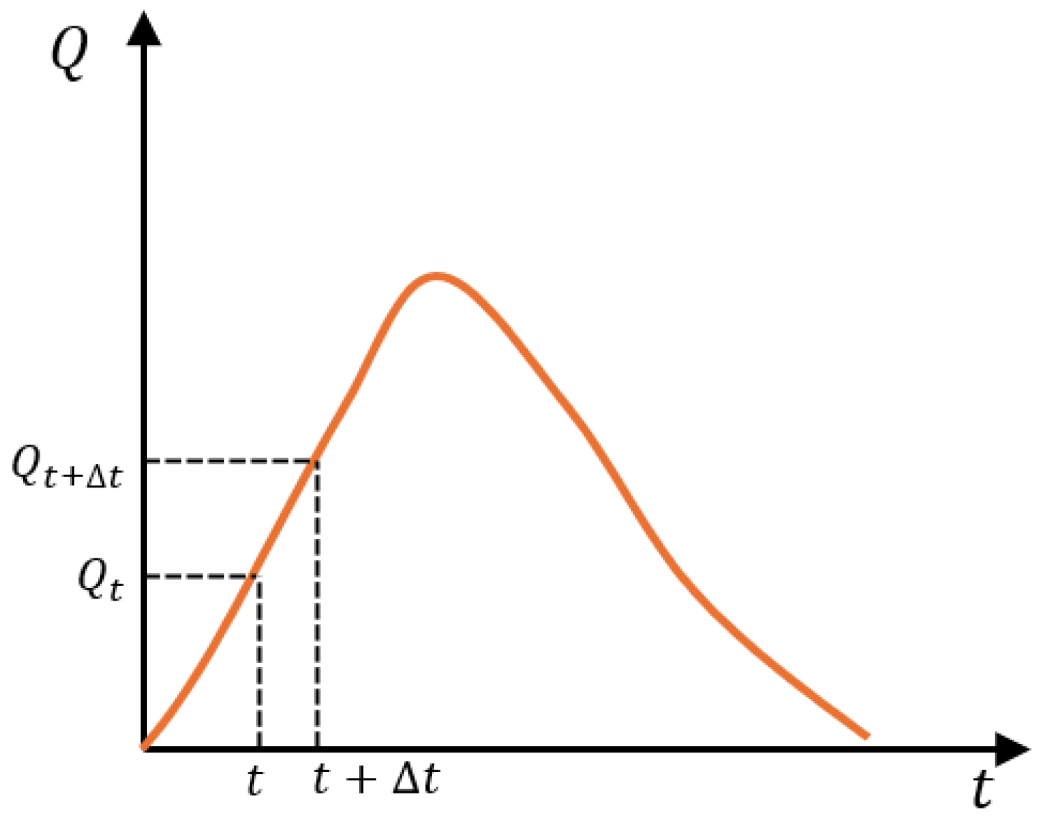
Considering the flow hydrograph depicted in Figure 1, the average flow rate for times $t$ and $t+∆t$ is determined by the following:

$$\overline{Q}=\frac{Q_t+Q_{t+∆t}}{2}$$

(1)

where $\overline{Q}$ = average flow rate for times $t$ and $t+∆t$, $Q_t$ = flow rate at $t$, and $Q_{t+∆t}$ = flow rate at $t+∆t$.

The volume ($V$) that is passing the time interval $∆t$ can be computed as follows:

$$V=\left(\frac{Q_t+Q_{t+∆t}}{2}\right)∆t$$

(2)

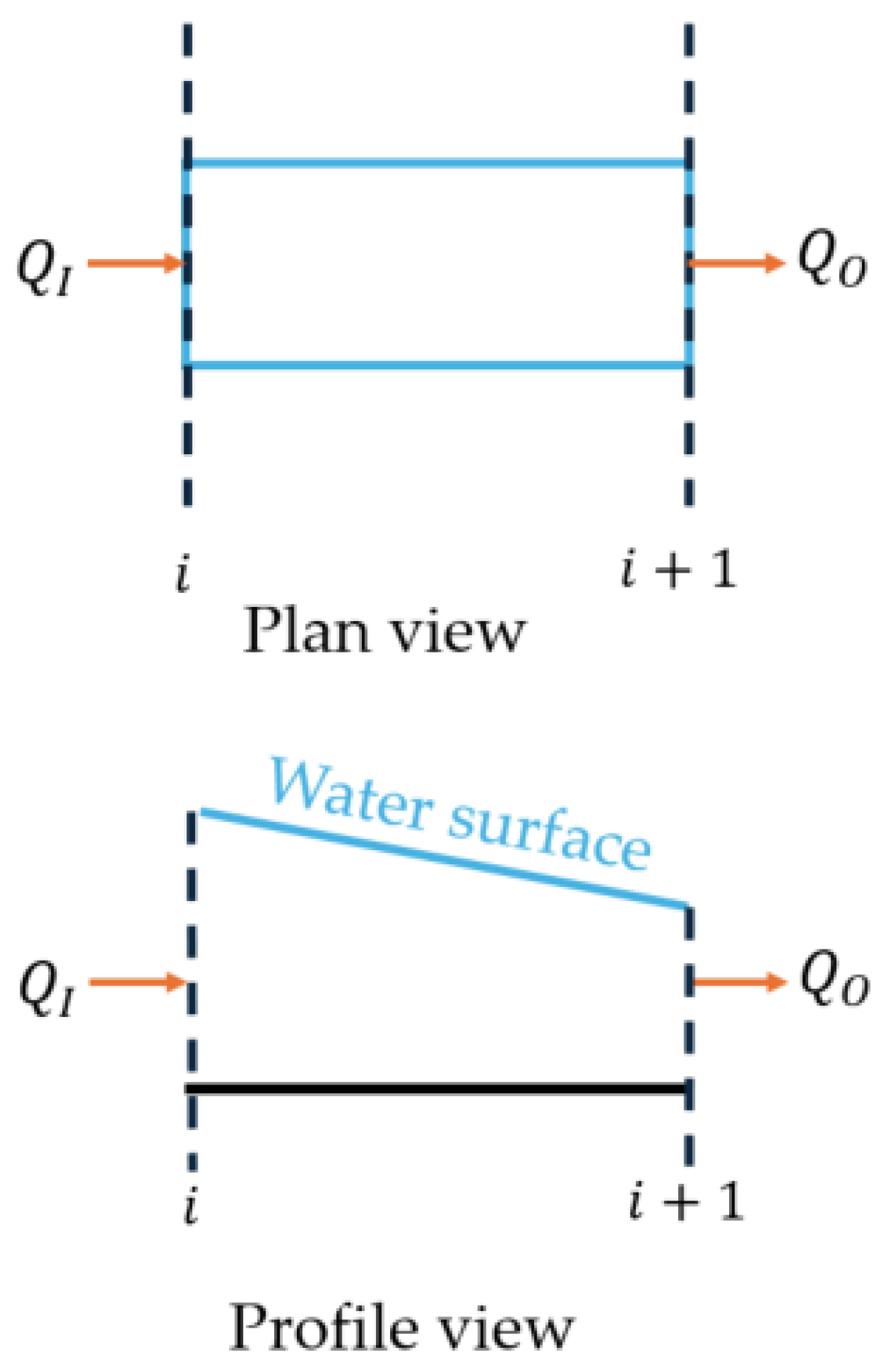
Now, considering a channel with two cross-sectional areas perpendicular to the flow (as shown in Figure 2), located at chainages $i$ and $i+1$, the following relationship can be established by considering the conservation of mass equations over the time interval $∆t$. Equation (3) is derived from a lumped routing method, which considers both the inflow and outflow hydrographs and the storage volume.

$$\left(\frac{Q_{I,t}+Q_{I,t+∆t}}{2}\right)∆t-\left(\frac{Q_{O,t}+Q_{O,t+∆t}}{2}\right)∆t=∆y\overline{T}L$$

(3)

where $Q_I$= inflow hydrograph at chainage $i$, $Q_{O,t}$ = outflow hydrograph at chainage $i+1$, $\overline{T}$ = average top width of the cross-sectional areas at chainages $i$ and $i+1$, $L$ = length between sections $i$ and $i+1$, and $∆y$ = variation in depth of flow between sections $i$ and $i+1$.

Expanding upon Equation (3), is possible to determine the following:

$$Q_{I,t}+Q_{I,t+∆t}-Q_{O,t}=\left(\frac{2L}{∆t}\right)\overline{T}∆y+Q_{O,t+∆t}$$

(4)

Considering the following:

$$a=\left(\frac{2L}{∆t}\right) \overline{T}$$

(5)

and

$$C=Q_{I,t}+Q_{I,t+∆t}-Q_{O,t}$$

(6)

Thus, reorganizing terms in Equation (4):

$$Q_{O,t+∆t}=C-a∆y$$

(7)

Considering a backwater downstream occurrence for a time $t$, then the conservation of mass is expressed as follows:

$$\left(\frac{Q_{I,t}-Q_{I,t+∆t}}{2}\right)∆t-\left(\frac{Q_{O,t}-Q_{O,t+∆t}}{2}\right)∆t=∆y\overline{T}L$$

(8)

For this condition is possible to demonstrate the following:

$$Q_{O,t+∆t}=-(C-a∆y)$$

(9)

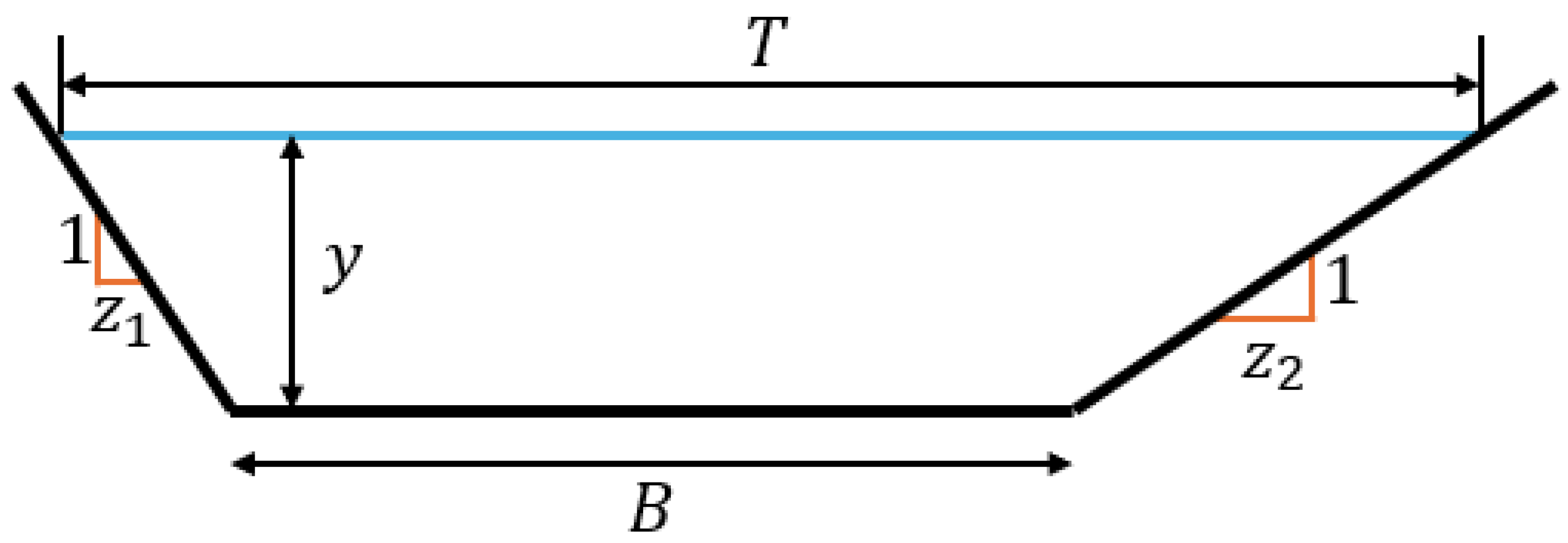
Given a trapezoidal channel as shown in Figure 3, then the flow area is given by the following:

$$A=By+\frac{1}{2}{y}^2\left(z_1+z_2\right)$$

(10)

where $A$ = flow area, $B$ = width of a cross-sectional, $y$ = depth of flow, $z_1=$ left side slope, and $z_2$= right side slope.

The analysis of a trapezoidal section involves the examination of values for $z_1$ and $z_2$. When $z_1$ and $z_2$ both equal 0, a rectangular cross-sectional area is depicted. Conversely, when $B$ equals 0, a triangular section is formed. This suggests that the proposed model has been developed considering these cross-sectional areas.

Now, if $K=(z_1+z_2)/2$, then:

$$A=By+K\ast y^2$$

(11)

Then, the top width can be expressed as follows:

$$T=B+2Ky$$

(12)

The wetted perimeter ($P$) for a trapezoidal section, featuring distinct left and right side slopes, is expressed as follows:

$$P=B+y\left(\sqrt{z_1^2+1}+\sqrt{z_2^2+1}\right)$$

(13)

Considering that $J=\sqrt{z_1^2+1}+\sqrt{z_2^2+1}$, then:

$$P=B+Jy$$

(14)

According to Manning’s equation, friction losses in a channel branch can be computed as follows:

$$Q=\frac{1}{n}\frac{A^{5/3}}{P^{2/3}}{S}^{1/2}$$

(15)

where $Q$ = water flow, $n$ = Manning’s coefficient, and $S$ = bed slope of a channel.

Substituting Equations (11) and (14) into Equation (15), then:

$$Q=\frac{1}{n}\frac{{(By+K{y}^2)}^{5/3}}{{(B+Jy)}^{2/3}}{S}^{1/2}$$

(16)

Using $b=S^{1/2}/n$, then Equation (16) is expressed for a time $t$ as follows:

$$Q_t=b\frac{{(By+K{y}^2)}^{5/3}}{{(B+Jy)}^{2/3}}$$

(17)

For a time $t+∆t$, the depth of flow is giving by $y+∆y$, thus:

$$Q_{t+∆t}=b\frac{{\left[B\right(y+∆y)+K{\left(y+∆y\right)}^2]}^{5/3}}{{[B+J\left(y+∆y\right)]}^{2/3}}$$

(18)

Considering a variable $M={\left[B\right(y+∆y)+K{\left(y+∆y\right)}^2]}^{5/3}$ and applying the binomial theorem for ${(y+∆y)}^2$, then:

$$M={\left[By+B∆y+K{y}^2+2Ky∆y+{K∆y}^2\right]}^{5/3}$$

(19)

Neglecting the term ${∆y}^2$:

$$M={\left[By+K{y}^2+(B+2Ky)∆y\right]}^{5/3}$$

(20)

If $D=By+K{y}^2$ and $E=B+2Ky$, then Equation (20) is expressed as follows:

$$M={\left[D+E∆y\right]}^{5/3}$$

(21)

In Equation (18), the denominator is giving by a variable $N={[B+J\left(y+∆y\right)]}^{2/3}$. If $F=B+Jy$, then is possible to demonstrate the following:

$$N=F^{2/3}+\frac{2}{3}{F}^{-1/3}J∆y$$

(22)

Inserting Equations (21) and (22) into Equation (18):

$$Q_{t+∆t}=b\left[\frac{D^{5/3}+\frac{5}{3}{D}^{2/3}E∆y}{F^{2/3}+\frac{2}{3}{F}^{-1/3}J∆y}\right]$$

(23)

Replacing Equation (23) into Equation (7), thus:

$$C-a∆y=b\left[\frac{D^{5/3}+\frac{5}{3}{D}^{2/3}E∆y}{F^{2/3}+\frac{2}{3}{F}^{-1/3}J∆y}\right]$$

(24)

Expanding Equation (24):

$$b{D}^{5/3}+\frac{5}{3}{D}^{2/3}bE∆y=C{F}^{2/3}+\frac{2}{3}{F}^{-1/3}CJ∆y-a∆y{F}^{2/3}-\frac{2}{3}{F}^{-1/3}Ja{∆y}^2$$

(25)

If the term ${∆y}^2\approx 0$, then:

$$∆y\left(\frac{5}{3}{D}^{2/3}bE-\frac{2}{3}{F}^{-1/3}CJ+a{F}^{2/3}\right)=C{F}^{2/3}-b{D}^{5/3}$$

(26)

Finally, for channel routing without accounting for backwater effects:

$$∆y=\left[\frac{C{F}^{2/3}-b{D}^{5/3}}{\frac{5}{3}{D}^{2/3}bE-\frac{2}{3}{F}^{-1/3}CJ+a{F}^{2/3}}\right]$$

(27)

Similarly, for the condition of backwater downstream occurrence, considering Equations (9) and (23), then:

$$∆y=\left[\frac{C{F}^{2/3}+b{D}^{5/3}}{a{F}^{2/3}-\frac{2}{3}{F}^{-1/3}CJ-\frac{5}{3}{D}^{2/3}bE}\right]$$

(28)

Considering that the formulation of the proposed model (see Section 2.1.2) is based on the Manning equation, it can be applied to calculate composite roughness, wherein the wetted area is divided into $N_p$ parts. Table 2 presents the various formulas for computing the equivalent roughness, depending on whether water velocities remain constant or vary within an analyzed cross-sectional area [29].

Table 2. Calculation of composite roughness in open channels.

Composite Roughness Formula	Application	Equation
$n={\left(\frac{\sum _1^{N_p}{P}_{N_p}{n}_{N_p}^{1.5}}{P}\right)}^{2/3}$	This formula applies to channels of suitable dimensions with varying Manning’s coefficients, provided no flooding exists. Consequently, each segment of the cross-sectional area experiences an equivalent average velocity.	(29)
$n=\frac{P{R}^{2/3}}{{\sum }_1^{N_p}\left(\frac{P_{N_p}{R}_{N_p}^{5/3}}{n_{N_p}}\right)}$	This equation is employed for channels containing floodplain zones, where different Manning coefficients and disparate water velocity distributions are observed.	(30)

Table 2. Calculation of composite roughness in open channels.

Composite Roughness Formula	Application	Equation
$n={\left(\frac{\sum _1^{N_p}{P}_{N_p}{n}_{N_p}^{1.5}}{P}\right)}^{2/3}$	This formula applies to channels of suitable dimensions with varying Manning’s coefficients, provided no flooding exists. Consequently, each segment of the cross-sectional area experiences an equivalent average velocity.	(29)
$n=\frac{P{R}^{2/3}}{{\sum }_1^{N_p}\left(\frac{P_{N_p}{R}_{N_p}^{5/3}}{n_{N_p}}\right)}$	This equation is employed for channels containing floodplain zones, where different Manning coefficients and disparate water velocity distributions are observed.	(30)

2.2. Current Channel Routing Methods

The proposed model underwent comparison with traditional methods as delineated in Table 3. Lumped and distributed channel routing methods were performed in this research.

Table 3. Current channel routing methods.

Channel Routing Method	Formulation	Equation No.	Observations
Lag model	$Q_{O,t}=\left\{\begin{array}{lll}{Q}_{I,t}& \mathrm{f}\mathrm{o}\mathrm{r}& t<t_{lag}\\ Q_{I,t+t_{lag}}& \mathrm{f}\mathrm{o}\mathrm{r}& t\ge t_{lag}\end{array}\right.$ where $t_{lag}$ = lag time.	(31)	The simplest method for hydrological routing.
Kinematic Wave	$Q_{i+1}^{j+1}=\frac{\frac{∆t}{∆x}{Q}_i^{j+1}+\alpha \beta Q_{i+1}^j{\left(\frac{Q_{i+1}^j+Q_i^{j+1}}{2}\right)}^{\beta -1}}{\frac{∆t}{∆x}+\alpha \beta {\left(\frac{Q_{i+1}^j+Q_i^{j+1}}{2}\right)}^{\beta -1}}$ where $\alpha ={\left(\frac{n{P}^{2/3}}{S^{1/2}}\right)}^{3/5}, \mathrm{and} \beta =0.6$.	(32)	$\mathrm{The} \mathrm{numerical} \mathrm{resolution} \mathrm{is} \mathrm{conducted} \mathrm{using} \mathrm{a} \mathrm{x}\text{–}\mathrm{y} \mathrm{plane}, \mathrm{where} \mathrm{an} \mathrm{unknown} \mathrm{flow} Q_{i+1}^{j+1}$$\mathrm{is} \mathrm{computed} \mathrm{based} \mathrm{on} \mathrm{known} \mathrm{flows} (Q_i^j$$, Q_{i+1}^j$$, \mathrm{and} Q_i^{j+1}$$) \mathrm{considering} \mathrm{appropriate} \mathrm{time} (∆t$$) \mathrm{and} \mathrm{space} (∆x$) steps.
Muskingum model	$S_t=K{Q}_{O,t}+K_{t}X(Q_{I,t}-Q_{O,t})$ where $S_t$ = storage at time $t$, $K_t$ = travel time in a channel (or storage constant), and $X$ = dimensionless weight.	(33)	This practical method requires the calibration of $K_t$$\mathrm{and} X$ parameters for performing accurate simulations.
Muskingum–Cunge model	$\frac{\partial Q}{\partial t}+c\frac{\partial Q}{\partial x}=\mu \frac{{\partial }^{2}Q}{\partial x^2}+c{q}_L$ where $c$ = wave celerity, $\mu$ = hydraulic diffusivity, an $q_L$ = lateral inflow (if applicable)	(34)	The hydraulic diffusitivity depends on hydraulic parameters.

Table 3. Current channel routing methods.

Channel Routing Method	Formulation	Equation No.	Observations
Lag model	$Q_{O,t}=\left\{\begin{array}{lll}{Q}_{I,t}& \mathrm{f}\mathrm{o}\mathrm{r}& t<t_{lag}\\ Q_{I,t+t_{lag}}& \mathrm{f}\mathrm{o}\mathrm{r}& t\ge t_{lag}\end{array}\right.$ where $t_{lag}$ = lag time.	(31)	The simplest method for hydrological routing.
Kinematic Wave	$Q_{i+1}^{j+1}=\frac{\frac{∆t}{∆x}{Q}_i^{j+1}+\alpha \beta Q_{i+1}^j{\left(\frac{Q_{i+1}^j+Q_i^{j+1}}{2}\right)}^{\beta -1}}{\frac{∆t}{∆x}+\alpha \beta {\left(\frac{Q_{i+1}^j+Q_i^{j+1}}{2}\right)}^{\beta -1}}$ where $\alpha ={\left(\frac{n{P}^{2/3}}{S^{1/2}}\right)}^{3/5}, \mathrm{and} \beta =0.6$.	(32)	$\mathrm{The} \mathrm{numerical} \mathrm{resolution} \mathrm{is} \mathrm{conducted} \mathrm{using} \mathrm{a} \mathrm{x}\text{–}\mathrm{y} \mathrm{plane}, \mathrm{where} \mathrm{an} \mathrm{unknown} \mathrm{flow} Q_{i+1}^{j+1}$$\mathrm{is} \mathrm{computed} \mathrm{based} \mathrm{on} \mathrm{known} \mathrm{flows} (Q_i^j$$, Q_{i+1}^j$$, \mathrm{and} Q_i^{j+1}$$) \mathrm{considering} \mathrm{appropriate} \mathrm{time} (∆t$$) \mathrm{and} \mathrm{space} (∆x$) steps.
Muskingum model	$S_t=K{Q}_{O,t}+K_{t}X(Q_{I,t}-Q_{O,t})$ where $S_t$ = storage at time $t$, $K_t$ = travel time in a channel (or storage constant), and $X$ = dimensionless weight.	(33)	This practical method requires the calibration of $K_t$$\mathrm{and} X$ parameters for performing accurate simulations.
Muskingum–Cunge model	$\frac{\partial Q}{\partial t}+c\frac{\partial Q}{\partial x}=\mu \frac{{\partial }^{2}Q}{\partial x^2}+c{q}_L$ where $c$ = wave celerity, $\mu$ = hydraulic diffusivity, an $q_L$ = lateral inflow (if applicable)	(34)	The hydraulic diffusitivity depends on hydraulic parameters.

It is of utmost importance to emphasize that the proposed model utilizes the variables of distributed routing methods—Manning’s coefficient, bed slope, cross-sectional area, and length of the channel branch—for channel routing computation despite being classified as a lumped model.

3. Results for a Practical Application

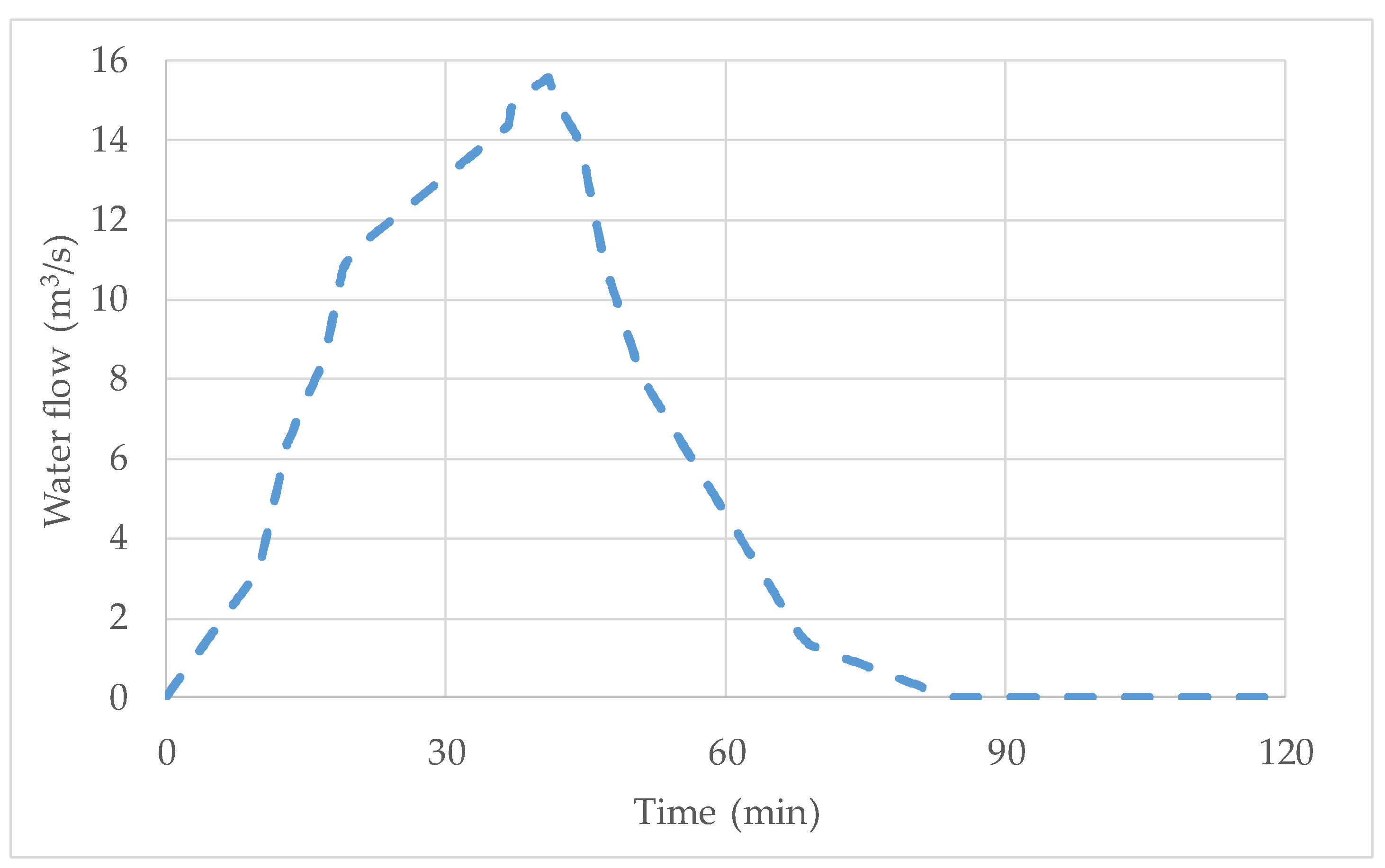
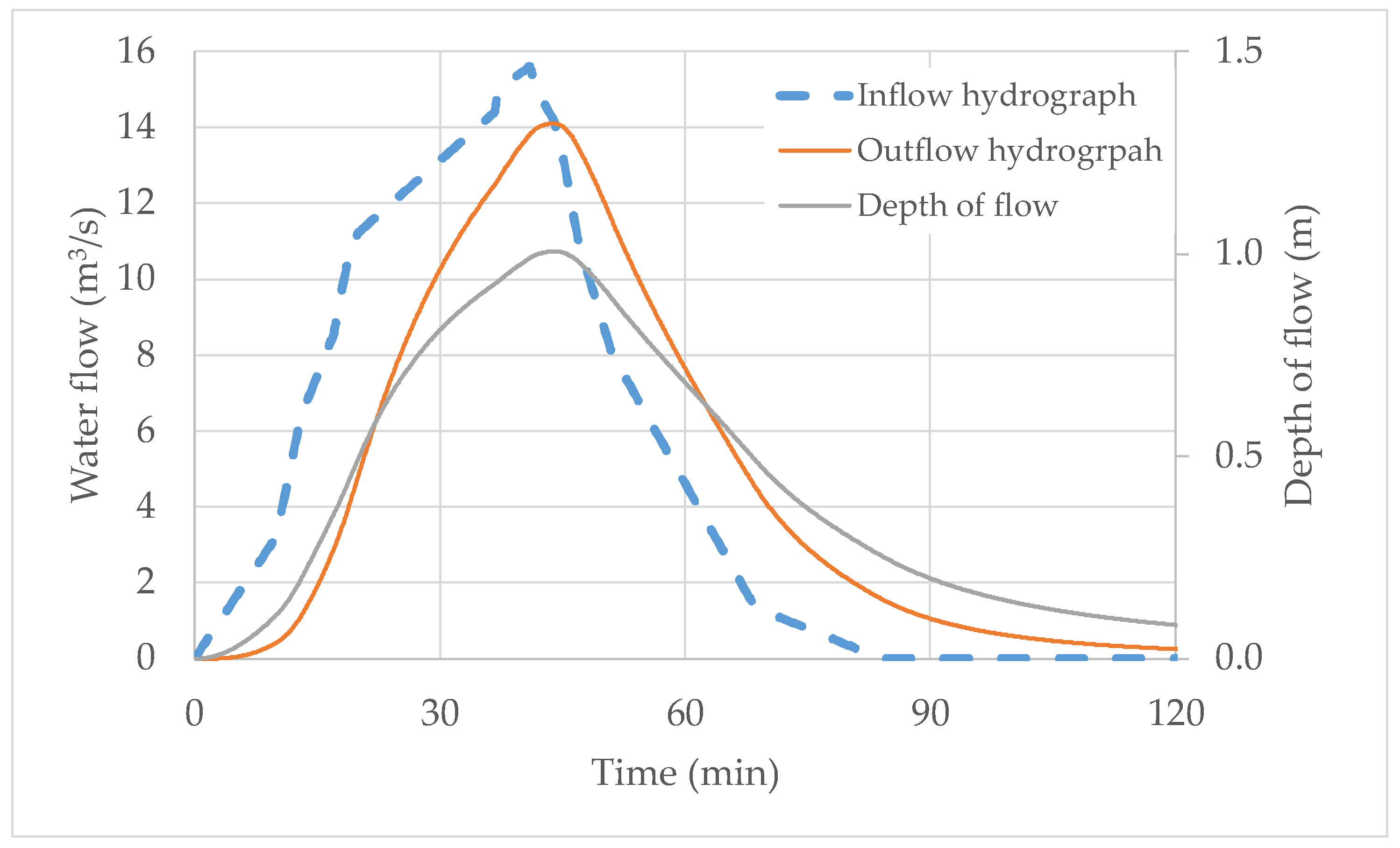
In order to examine the application of the proposed model, an open channel routing was carried out, focusing on a rectangular cross-sectional area. The following data were considered: $n=$ 0.015 (complete rectangular section), $S=$ 0.12%, $B=$ 7.0 m, $z_1=z_2=0$, and $L=$ 1200 m. A time step ($∆t$) of 0.25 min was used for simulations. The inflow hydrograph is presented in Figure 4, showing a peak flow of 15.56 m³/s occurring at 40.75 min. The total duration of the inflow hydrograph is 83.75 min.

The channel routing is executed employing the proposed model outlined in Section 2.2. Figure 5 illustrates the outcomes of the channel routing. The peak value of the outflow hydrograph is 14.10 m³/s, observed at 44.0 min, shifting by 3.5 min compared to the inflow hydrograph. Under these conditions, the outflow hydrograph lasts around 120 min, presenting a maximum flow depth of 1.00 m. The depth of the flow pattern aligns with the outflow hydrograph as these variables are interconnected.

A sensitivity analysis was conducted, varying the critical parameters of the proposed model.

Table 4. Considered parameters for the sensitivity analysis.

Parameter	Units	Range
		From	To
$\mathrm{Manning}\prime \mathrm{s} \mathrm{coefficient} \left(n\right)$	-	0.013	0.017
$\mathrm{Bed} \mathrm{slope} \left(S\right)$	%	0.06	4.00
Width of the open channel $\left(B\right)$	m	4	20

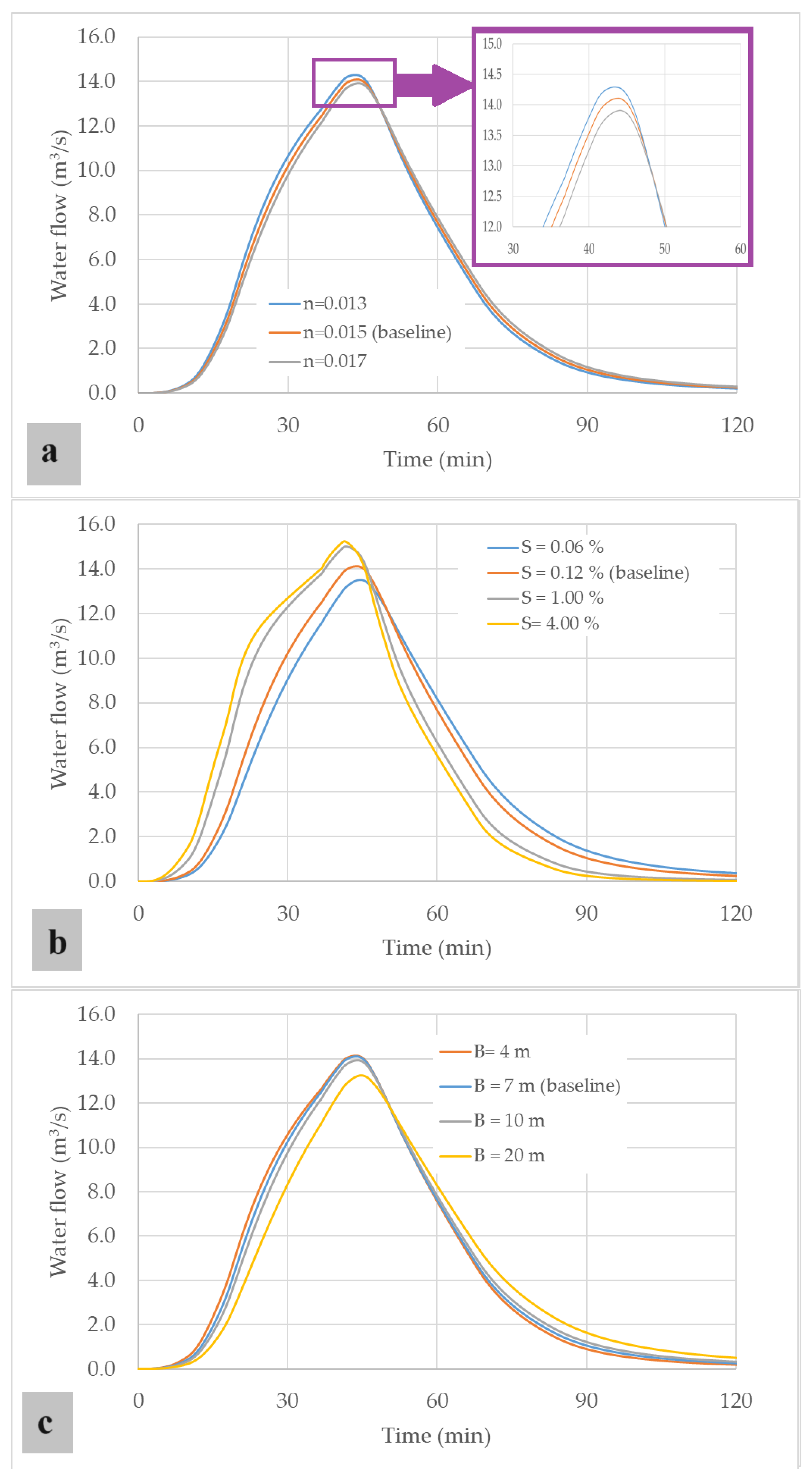
outlines the parameters considered for the analysis, including Manning’s coefficient ($n$), bed slope ($S$), and width of the open channel ($B$). Figure 6 illustrates the outcomes. A comparison is made of the results of the outflow hydrograph. The initial data (Figure 5) is labeled as the baseline solution in Figure 6.

The impact of Manning’s coefficient on the outflow hydrograph is evident in Figure 6a. A lower Manning’s coefficient corresponds to higher peak flow values. For example, with $n$ = 0.013, a peak value of 14.29 m³/s is reached, while with $n$ = 0.017, a value of 13.91 m³/s is obtained. Generally, within a reasonable range, variations in Manning’s coefficient do not significantly influence the pattern of the outflow hydrograph.

The bed slope ($S$) can markedly alter the pattern of the outflow hydrograph, depending on the value considered, as demonstrated in Figure 6b. A greater bed slope leads to higher peak flow values and earlier peak times. For a slope of 4.00%, a maximum flow value of 15.24 m³/s is attained at 41.5 min, closely resembling the inflow hydrograph (Figure 4), since steep slopes cannot retain sufficient water volume within the 1200 m length considered. Conversely, mild bed slopes tend to store significant water volume during open channel routing, as observed with a slope of 0.06%, where the resulting peak value is 13.52 m³/s at 44.5 min, indicating a reduction of around 13.0% compared to the peak value of the inflow hydrograph (15.56 m³/s).

The width of the open channel varied from 4 to 20 m. Higher width values correspond to lower peak flow values. For instance, with a width ($B$) of 4 m, a peak flow value of 14.15 m³/s is observed, whereas with $B$ = 20 m, it decreases to 13.23 m³/s.

4. Discussion

In this section, an examination of the proposed model has been undertaken. Initially, the time step was varied by adding 1.00 and 5.00 min increments. Figure 7 illustrates the findings, demonstrating that employing a time step of 0.25 (refer to Section 3) and 1.00 min yields comparable peak flows and analogous water pulses. Conversely, a slight beat disparity emerges when a time step of 5 min is utilized. Notably, a maximum water flow of 13.99 m³/s is calculated for this time step, in contrast to a peak value of 14.10 m³/s (for $∆t$ = 0.25 min). Furthermore, the peak time is advanced, occurring at 40.0 min (for $∆t$ = 5.00 min) as opposed to the timing of 43.5 min (for $∆t$ = 0.25 min).

The results of the proposed model were subject to a comparative evaluation against the lumped and distributed methods outlined in Table 1 for practical application.

Table 5. Characteristics of the different channel routing methods.

Channel Routing Method	Considerations	Used Parameters
Lag model	The lag time was computed based on the consideration of the storage constant in the Muskingum model.	Lag time ($t_{lag}$ = 13.2 min)
Kinematic Wave	The celerity index method was utilized, considering an index celerity ($C_{index}$) of 1.52 m/s. The number of branches was 4.	$n=$$0.015, S=$$0.12\%, B=$$7.0 \mathrm{m}, L=$$1200 \mathrm{m}, \mathrm{and} C_{index}$ = 1.52 m/s
Muskingum model	The calculation of the storage constant ($K_t$) is founded upon a bankfull water velocity $\left(v\right)$ of 0.91 m/s, computing wave celerity as $c$ = $1.67v$ = 1.52 m/s.	$K_t$ = 0.22 h and $X$ = 0.2
Muskingum–Cunge model	For the simulations, the values of $∆t$ and $∆x$ were automatically selected by the software. An index flow ($Q_{index}$) of 15.6 m3/s is established as the maximum flow.	$n=$$0.015, S=$$0.12\%, B=$$7.0 \mathrm{m}, L=$$1200 \mathrm{m}, \mathrm{and} Q_{index}$ = 15.6 m3/s

delineates the factors considered in calculations, encompassing Lag, Kinematic Wave, Muskingum, and Muskingum–Cunge models, along with the parameters utilized, simulated via the HEC-HMS software (Version 4.12).

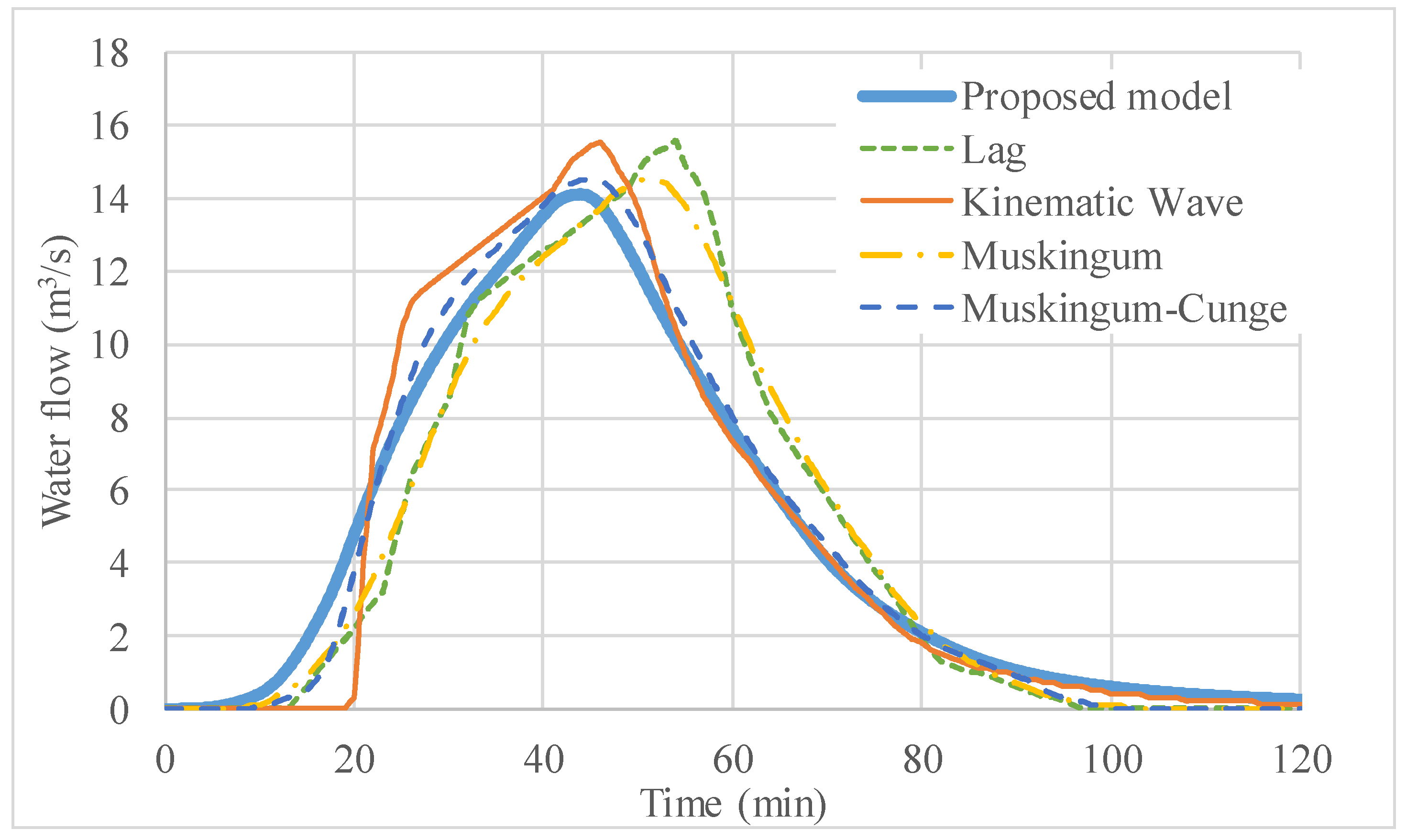
Figure 8 compares outflow hydrographs between the proposed model and the lumped and distributed models. The Muskingum method yields values akin to the proposed models, with peak water flows of 14.5 and 14.1 m³/s computed, respectively, exhibiting a discrepancy in peak time of 3 min. The Muskingum–Cunge method yields the closest values related to the peak flow, with 14.5 m³/s occurring at 44 min. Across all simulations, the Kinematic Wave and Lag methods yield higher peak water flows than those predicted by the proposed model. It is essential to mention that the proposed model (a lumped routing method) provides values similar to those of the Muskingum–Cunge (a distributed routing method).

A comparative analysis was conducted between the proposed model and other lumped and distributed models, considering the attributes outlined in Table 1. The proposed model operates as a lumped channel routing technique akin to Lag and Muskingum models. It is a pragmatic approach, leveraging typical hydraulic parameters such as Manning’s coefficient, bed slope, geometric cross-sectional area characteristics, and channel branch length to facilitate the routing of an inflow hydrograph while accommodating backwater effects. Unlike the Muskingum model, the proposed model does not rely on intricate parameters for determination. In contrast, it necessitates hydraulic parameters like those required by distributed models such as the Kinematic Wave and Muskingum–Cunge models. This renders it applicable for both mild and steep bed slopes without the need for adherence to a Courant condition, as it is not a distributed model. The Muskingum–Cunge method has yielded more precise outflow hydrograph computations than other hydrological and hydraulic methods [30].

The Root Mean Square Error (RMSE) was calculated for the outflow hydrographs, considering both lumped and distributed models (refer to Figure 8). The Muskingum–Cunge method was employed as the reference values. Subsequently, the RMSE was determined as follows:

$$RMSE=\sqrt{\frac{1}{N}{\left(C-O\right)}^2}$$

(35)

where $C$ represents the computed values obtained from the proposed model, Lag, or Muskingum methods, $O$ corresponds to the observed values (in this instance, using the Muskingum–Cunge method), and $N$ denotes the number of observations modelled.

Table 6. Computation of Mean Square Error.

Method	RMSE (m3/s)	Observation
Proposed model	0.53	-
Muskingum	1.34	-
Kinematic Wave	0.64	-
Lag	1.45	-
Muskingum–Cunge	-	This method was considered as reference values

displays the RMSE results. The proposed model exhibited the best accuracy compared to the Lag, Muskingum, and Kinematic Wave methods, underscoring its significance as a novel mathematical model for channel routing since the lowest value of RMSE was obtained (0.53 m³/s).

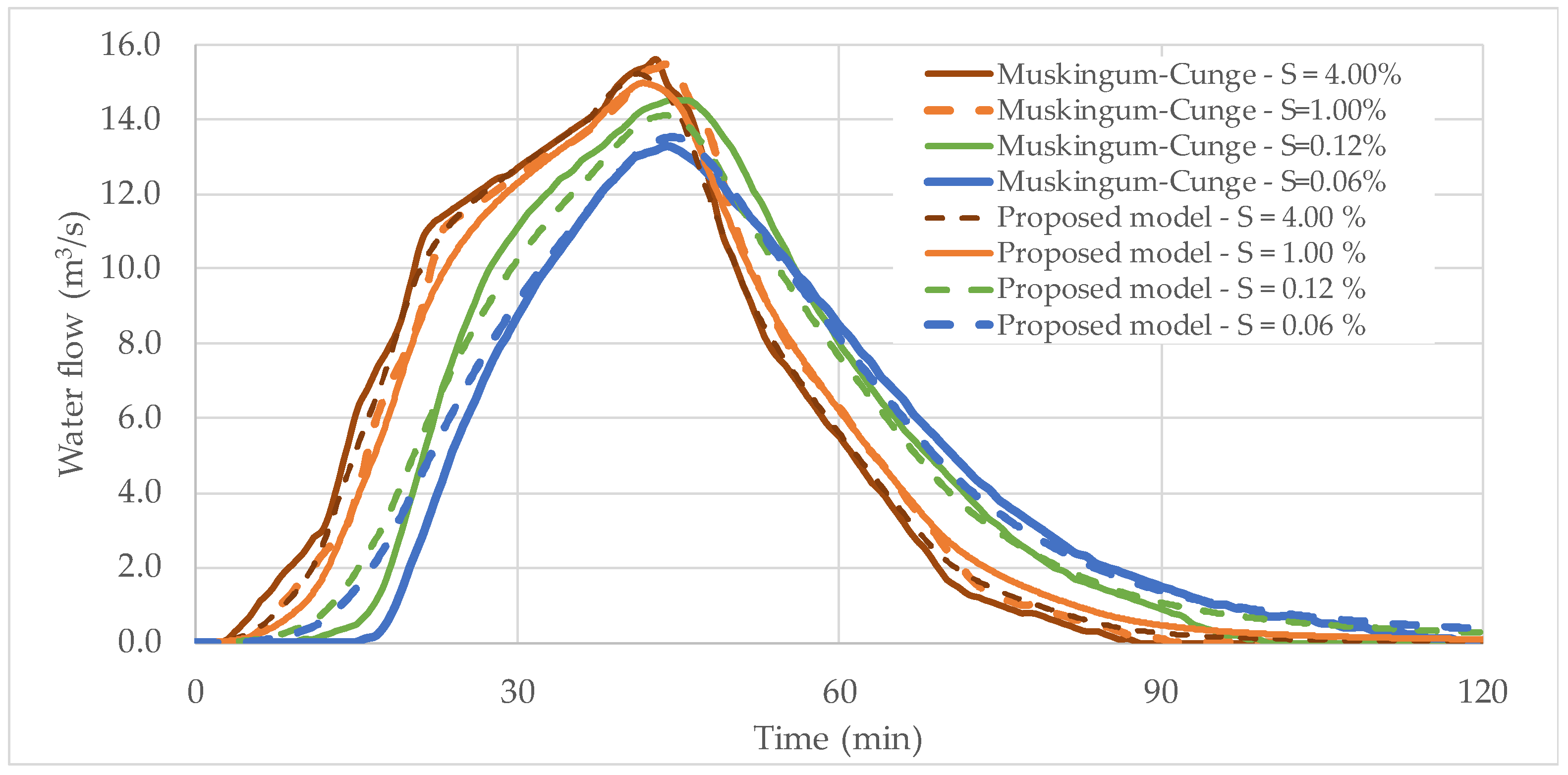
The bed slope is the most sensitive parameter for channel routing, as depicted in Figure 6b. Considering this, the results of the proposed model were contrasted with those of the Muskingum–Cunge method across bed slopes ranging from 0.06 to 4.0%. Figure 9 illustrates the outcomes, indicating that the proposed model (a lumped routing model) yielded comparable values to the Muskingum–Cunge method (a distributed routing model). This demonstrates the applicability of the proposed model as an explicit scheme, with the significant advantage of requiring less computational time than the Muskingum–Cunge method.

5. Conclusions

Channel routing methods have developed significantly to determine the transformation of an inflow hydrograph along a channel branch to ascertain the resultant conditions (outflow hydrograph). These methods typically fall into two categories: lumped and distributed models. Some models overlook critical terms, while others fail to account for backwater effects. Additionally, specific models rely on complex parameters that necessitate calibration for accurate determination.

This study devised a novel channel routing method rooted in the principles of mass conservation and Manning equations. This method is versatile and can accommodate both steep and mild bed slopes. It employs standard hydraulic parameters—including Manning’s coefficient, bed slope, geometric cross-sectional area characteristics, and channel branch length—throughout its calculations and incorporates considerations for backwater effects. The proposed model is applicable for channels with bed slopes lower than 6°.

To showcase the effectiveness of the proposed model, a practical application was undertaken, demonstrating its capabilities and yielding tangible results for a rectangular channel measuring 1200 m in total length and 7 m in width. This application considered a peak flow ranging from 15.6 to 14.1 m³/s, reflecting inflow and outflow hydrographs, respectively. A sensitivity analysis was conducted, varying Manning’s coefficient, bed slope, and the width of the open channel. The robustness of the proposed model was evident as variations in these parameters consistently influenced the generation of different outflow hydrographs.

The proposed model was compared with the Lag, Kinematic Wave, Muskingum, and Muskingum–Cunge models. The results of the proposed model reveal that it produces water flow oscillations within a similar range to existing models.

Future research should be focused on the assessment of the time-saving benefits offered by the proposed model compared to distributed routing models such as Kinematic Wave and Muskingum–Cunge. Furthermore, the implementation of an explicit scheme, akin to the proposed model, should be conducted while considering two-dimensional routing methods.