Article

A Study of Precipitation Forecasting for the Pre-Summer Rainy Season in South China Based on a Back-Propagation Neural Network

1
College of Hydrology and Water Resources, Hohai University, Nanjing 210098, China
2
China Meteorological Administration Hydrometeorology Key Laboratory, Nanjing 210098, China
3
College of Oceanography, Hohai University, Nanjing 210098, China
4
China Meteorological Administration, Beijing 100081, China
*
Authors to whom correspondence should be addressed.
Water 2024, 16(10), 1423; https://doi.org/10.3390/w16101423
Submission received: 31 March 2024 / Revised: 30 April 2024 / Accepted: 15 May 2024 / Published: 16 May 2024

Abstract

:
In South China, the large quantity of rainfall in the pre-summer rainy season can easily lead to natural disasters, which emphasizes the importance of improving the accuracy of precipitation forecasting during this period for the social and economic development of the region. In this paper, the back-propagation neural network (BPNN) is used to establish the model for precipitation forecasting. Three schemes are applied to improve the model performance: (1) predictors are selected based on individual meteorological stations within the region rather than the region as a whole; (2) the triangular irregular network (TIN) is proposed to preprocess the observed precipitation data for input of the BPNN model, while simulated/forecast precipitation is the expected output; and (3) a genetic algorithm is used for the hyperparameter optimization of the BPNN. The first scheme reduces the mean absolute percentage error (MAPE) and the root mean square error (RMSE) of the simulation by roughly 5% and more than 15 mm; the second reduces the MAPE and RMSE by more than 15% and 15 mm, respectively, while the third improves the simulation inapparently. Obviously, the second scheme raises the upper limit of the model simulation capability greatly by preprocessing the precipitation data. During the training and validation periods, the MAPE of the improved model can be controlled at approximately 35%. For precipitation hindcasting in the test period, the anomaly rate is less than 50% in only one season, and the highest is 64.5%. According to the anomaly correlation coefficient and Ps score of the hindcast precipitation, the improved model performance is slightly better than the FGOALS-f2 model. Although global climate change makes the predictors more variable, the trend of simulation is almost identical to that of the observed values over the whole period, suggesting that the model is able to capture the general characteristics of climate change.

1. Introduction

The pre-summer rainy season (April to June) is referred to as the first rainy period of the year in contrast to the second rainy period (July to September) in South China [1]. The average precipitation during this period is 665 mm, accounting for approximately 50% of the annual total. Some studies have shown that the average number of rainstorm days in the pre-summer rainy season accounts for half of that in the whole year [2]. The long-term and widespread rainfall is characterized by its high intensity and volume, which can easily lead to natural disasters such as mountain flooding, landslides, and urban flooding [3], posing a threat to people’s lives and property. Therefore, it is of great importance to improve the accuracy of precipitation forecasting during the pre-summer rainy season in South China.
Located in the coastal region, South China has complicated topography. The weather systems controlling this area during the pre-summer rainy season are complex [4], in which many general circulation patterns or antecedent factors affect precipitation, making it difficult for models to describe land–atmosphere interactions and then forecast the precipitation over the region. To investigate the physical processes involved, a number of researchers have carried out numerous studies using available observation and reanalysis data or by methods of numerical simulation. Qiang et al. [5] studied the sudden changes in precipitation and atmospheric circulation indices at the beginning and end of the pre-summer rainy season. Li et al. [6] analyzed the statistical characteristics of precipitation during different periods of the pre-summer rainy season (frontal precipitation period and monsoon precipitation period). Chen et al. [7] carried out numerical simulation experiments to investigate the effect of the sea surface temperature (SST) in the Western Pacific warm pool region on pre-summer precipitation. In addition, the relationship between the precipitation and some indices of the atmosphere [8,9,10], oceans [11,12], and the land surface [13] has also been studied so that the choice of predictors has a relatively physical foundation when setting up statistical precipitation forecasting models.
Methods for precipitation forecasting are mainly classified into statistical and dynamical groups [14,15]. In recent years, there have been a great number of studies using numerical models based on dynamical methods, e.g., the regional climate model RegCM3 and the climate forecast system CFSv2, to forecast precipitation in different regions of South China at different time scales of the pre-summer rainy season [16,17,18,19]. Based on these studies, it can be found that the error of the forecast of numerical models increases with the lead time; various numerical models are highly skilled in precipitation forecasting in some regions of South China, but their forecast capability is weak systematically over the whole area. Meanwhile, some studies employed traditional statistical methods, e.g., the singular value decomposition method [20], the partial least squares regression methods [21], and the canonical correlation analysis method [22], to forecast precipitation during the per-summer rainy season. Statistical methods are more suitable for seasonal scale precipitation forecasting [23,24], but it is difficult to predict the precipitation distribution with higher resolution. In general, both dynamic and traditional statistical methods for pre-summer precipitation forecasting in South China have been developing in the past two decades, but few studies can predict both accurate total amounts of seasonal precipitation and reasonable spatial distributions of the precipitation during the pre-summer rainy season.
As a feed-forward network based on the error back-propagation algorithm, the back-propagation neural network (BPNN) is one of the most widely used artificial neural networks [25,26]. In the last two decades, the BPNN has been widely used in precipitation forecasting. Compared with dynamical methods, the BPNN is more fault-tolerant; compared with traditional statistical methods, the BPNN does not require the mastery of a priori statistical laws [27]. Many studies have confirmed that it is a stable and effective method [28,29,30]. Previous researchers [31,32] confirmed that the BPNN optimised by a genetic algorithm performs better than the multiple linear regression (MLR) method in different areas. This study demonstrates the feasibility that BPNN can predict not only the amount of precipitation but also the spatial distribution skillfully. As with most artificial neural networks, the error of BPNN simulation comes from three main sources: weakness of model structure, poor internal characteristics of the data, and unoptimised hyperparameters. The internal characteristics of data determine the upper limit of BPNN simulation capability. Conventional data preprocessing methods, e.g., wavelet denoising and mean filtering, can make the characteristics of data more prominent and remove the noises [33]. Aiming at improving the simulation of the BPNN in this paper, a method for preprocessing precipitation data based on the triangular irregular network (TIN) is introduced.
Additionally, under the background of global climate change, temperatures worldwide are rising, and the state of the atmosphere is becoming more nonstationary [34], causing transformations to the physical processes involved in precipitation. In the field of hydrological forecasting, once the regional climate of an area has changed, the inconsistency of the hydrological sequence in the area affects the hydrological data and the hydrological model parameters, making them no longer representative [35]. Thus, the hydrological model needs to be calibrated repeatedly to ensure accuracy and reliability due to global climate change. This paper discusses whether the same problem exists in the precipitation forecasting model based on BPNN, finding out whether the BPNN is able to capture the changed physical processes automatically or by calibration.
This paper attempts to set up a precipitation forecasting model based on BPNN for the pre-summer rainy season in South China. There are three schemes to improve the model according to the three sources of the BPNN simulation error. The improved models are used to hindcast the precipitation so that their performance can be evaluated. In Section 2 of this paper, data sources of precipitation, climate indices, and the hindcast precipitation of a dynamical climate model are introduced. Section 3 presents the approaches to set up the model, the schemes to improve the model, and the evaluation indices. The results are analyzed in Section 4, and the rest part of this paper contains a discussion and summary.

2. Data and Methods

2.1. Overview of the Experiments

The BPNN learns historical data from the training set to determine the network structure. The validation set is used for the judgment of overfitting and the optimization of hyperparameters, and finally, the determined network is applied in independent prediction during the test period. In this paper, the simulation refers to the model performance during the training and validation periods, and the hindcast is referred to the model performance during the test period. In consideration of the availability of data, the training set, validation set, and test set are divided according to the ratio 7:2:1, i.e., 1969–2002, 2003–2012, and 2013–2017. The simulation is influenced by data processing, model building, and hyperparameter optimization. After different methods of data preprocessing, the model is built based on BPNN, and the initial weights and biases of BPNN are optimised by a genetic algorithm (GA). The model with preeminent and reasonable simulation is applied in hindcasting. The experiments in this paper are designed according to four schemes (Table 1). They are described in detail in the following sections.

2.2. Data Sources and Processing

Precipitation data (the expected output of the model) are derived from the Daily Values of Terrestrial Climate Information in China dataset (V3.0). This dataset contains daily precipitation data from 824 national benchmarks and basic stations on the ground in China, with missing or mismeasured data in some stations. The study area of this paper is South China, including Guangdong, Guangxi, and Hainan provinces (104°26′ E–117°19′ E; 18°10′ N–26°24′ N); the study period is the pre-summer rainy season (April to June). Spatial interpolation is carried out for missing or mismeasured data for the area during the period. Considering the large number of missing or mismeasured data for some years and some stations, 93 stations (Figure 1) are finally chosen to participate in the model construction over 49 years, i.e., 1969–2017.
Climate index data (the inputs of the model) are derived from the 130 monthly monitoring indices from China National Climate Centre, including 88 indices for atmospheric circulation, 26 for sea surface temperature (SST), and 16 for other indices such as the total sunspot number index and the solar flux index (Supplementary Materials). Predictors are taken from the climate index data in the previous months before the pre-summer rainy season (i.e., December of the preceding winter to March).
Hindcast data of a dynamical model are obtained from the sub-seasonal to seasonal (S2S) prediction system built by the Institute of Atmospheric Physics, Chinese Academy of Sciences, based on the FGOALS-f2 model. Hindcast experiments have confirmed its high prediction skills for ENSO, the Madden Julian Oscillation (MJO), and tropical cyclones [36], and they have been incorporated into the China Multi-Model Ensemble (CMME) [37]. The data of the FGOALS-f2 model in raster format are spatially interpolated to obtain the values of the 93 stations. The hindcast data during 2013–2017 are selected and used for comparison with the hindcast precipitation of the model in this study.

2.3. Methods

2.3.1. Correlation Analysis

Correlation analysis is used for the selection of predictors. In this paper, Pearson’s correlation coefficients between the 130 monthly monitoring indices in the previous months before the pre-summer rainy season and the monthly precipitation series in the pre-summer rainy season are calculated separately. Monthly monitoring indices with significance levels higher than 0.05 are excluded, and the remains are listed in descending order of the absolute values of the correlation coefficients. Finally, the top four indices from different previous months are selected as the predictors in this paper.

2.3.2. Back-Propagation Neural Network (BPNN)

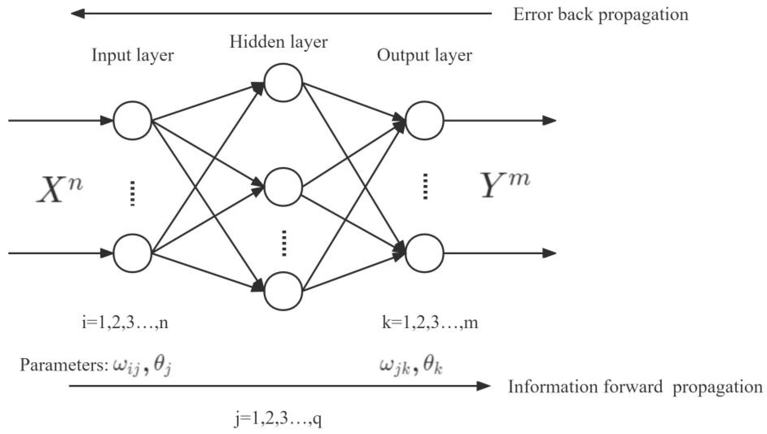
The BPNN is usually composed of an input layer, several hidden layers, and an output layer. The principle of BPNN can be briefly described as follows: the input X is combined linearly to obtain the total input S, the weight of the linear combination is ω, and the biase is θ; the total input S is acted upon by the activation function f to obtain the output P, which is usually a nonlinear function to fit a complex relationship; there exists a deviation E between the output P and the expected output O, which is a function of the weights and biases. The objective is to find the optimal weights and biases with the minimum deviation, and the method of seeking optimal values is usually the gradient descent method. Once the optimal weights and biases are determined, the structure of the BPNN is also determined, i.e., the BPNN completes its training and can be used for simulation or actual forecasting. Therefore, BPNN does not require a priori knowledge to spontaneously disclose the internal laws of the data. Figure 2 shows the structure of a conventional BPNN containing 1 hidden layer [38].
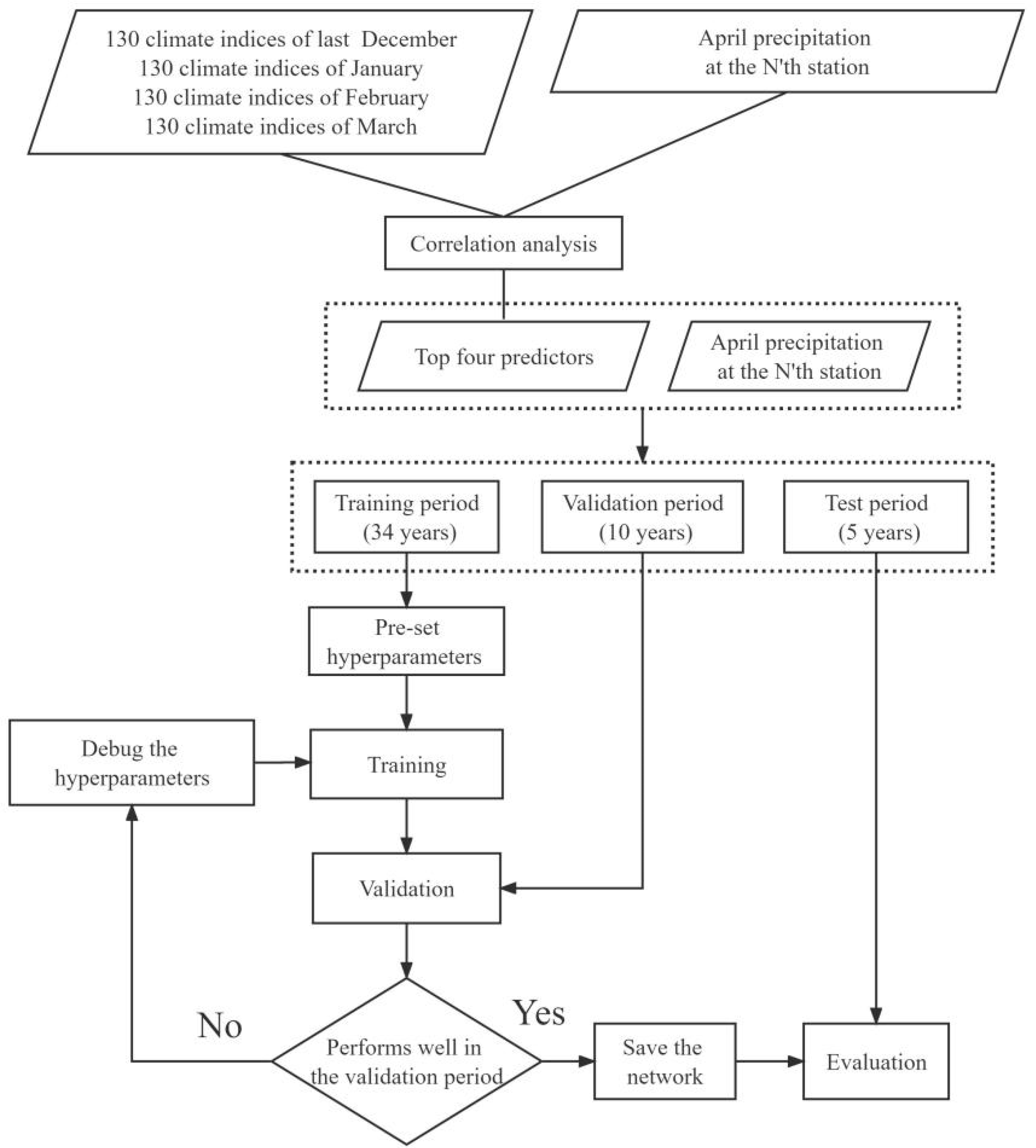
This paper attempts to establish a precipitation forecasting model for the pre-summer rainy season in South China. From the perspective of spatial scale, the region includes 93 stations; from the perspective of time scale, the pre-summer rainy season includes 3 months. Accordingly, the task of the model can be divided into sub-model tasks, each of which is an independent BPNN to realize the forecast of precipitation for a month at a station individually. For example, for the forecast of April precipitation at the Nth station, the expected output of the BPNN is April precipitation series at the station. There are two options for the inputs: the series of the top four climate indices most correlated with the regional mean precipitation series for April, which makes the model more interpretable, and the series of the top four climate indices most correlated with the precipitation series for April at the station, which theoretically improves the accuracy of the simulation. The flow charts (Figure 3 and Figure 4) show the sub-models for forecasting April precipitation at the Nth station for both options of inputs, which are noted as SregBP and SstnBP.
The hyperparameters that usually have significant impacts on the performance of BPNN are as follows: the number of hidden layer neurons, the activation function, the initial weights and biases, the learning rate, the number of epochs, and the error goal [39]. In this paper, the range for the number of hidden layer neurons is determined by Equation (1).
q = n + m + a ,
In the formula, q is the number of hidden layer neurons, n and m are the numbers of neurons in the input and output layers with the values of 4 and 1 in this study, and a is an integer ranging from 1 to 10. Different q values within the range are tested, and the q value that presents the best training effect is taken into the BPNN. In this paper, the number of hidden layer neurons and the activation function are unchanged once they are set and are not involved in debugging. The initial weights and biases are randomly generated from the interval [−1, 1]. The learning rate, the number of epochs, and the error goal require manual debugging. The network is trained using the 34 years of data (1969–2002). The trained network is used to simulate the precipitation in the validation period. The learning rate, the number of epochs, and the error goal are adjusted according to the error of simulation so that the network, after hyperparameter optimization, has the best performance in the validation period. The network structure is saved, which means the sub-model is established and can be used to hindcast precipitation for the test period.
For each sub-model, the four predictors are first selected according to correlations. The n, the neural network, is trained on the training set, and the hyperparameters are adjusted according to the validation set error. Finally, the network is saved and used for hindcast on the test set.
In practical application, the hyperparameters of each sub-model are adjusted separately, and the best hyperparameters can vary among sub-models. However, for convenience in this study, the hyperparameters of the sub-models are adjusted uniformly, i.e., the hyperparameters of 93 sub-models based on the stations remain consistent and share one set of values.

2.3.3. Triangular Irregular Network (TIN)

TIN is introduced to preprocess precipitation data (the expected output) in this study. Previously, TIN was widely used in digital elevation models to fit the ground surface or other irregular surfaces. The most conventional method of generating it is the Delaunay triangulation method [40]. TIN is similar to orthogonal grids in that it can simply be understood as a form of interpolation. The advantages of TIN over orthogonal grids are as follows. TIN node data are the original observed data, while orthogonal grid node data are the interpolated values of the original observed data. The topological relationship of TIN is better than that of orthogonal grids. It has been confirmed that TIN is more suitable for handling data with large spatial variability [41].
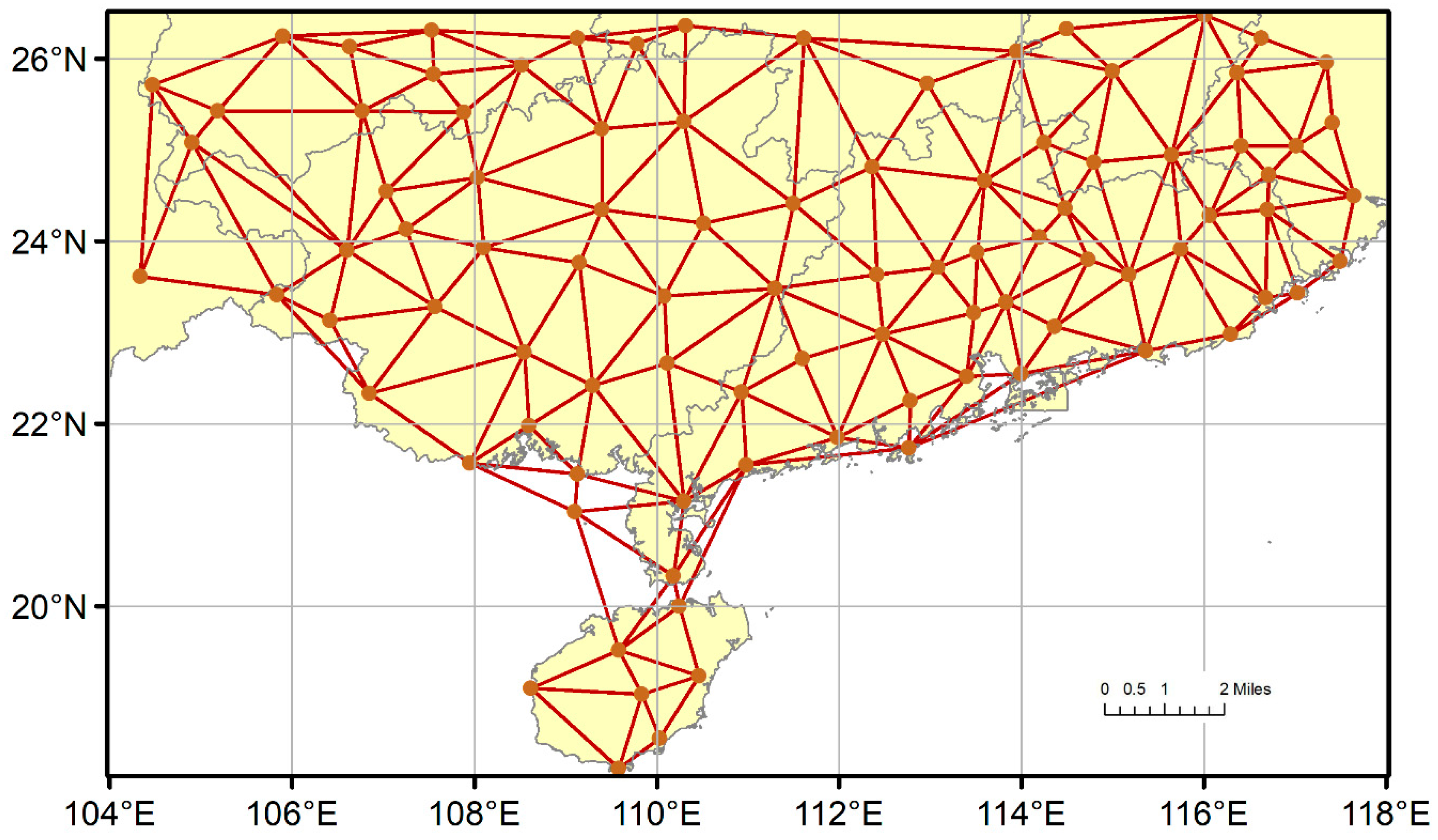
In this paper, a TIN is generated based on 93 stations in the region, including 154 triangular areas (Figure 5). Some unreasonable triangles are abandoned, which are mainly obtuse triangles located at the boundary of the region and spanning long distances.
The mean precipitation for each triangular area is an average of the precipitation at the three stations located on the apices of the triangle, i.e., an equally weighted linear combination of the precipitation at the three stations. Therefore, preprocessing by the TIN changes the internal characteristics of the precipitation data. To ensure that the preprocessing does not destroy the spatial distribution of precipitation, the annual average precipitation during the pre-summer rainy season is calculated for each of the 93 stations (denoted as PN, N = 1, 2, 3, ..., 93), and each of the 154 triangular regions (denoted as PM, M = 1, 2, 3, ..., 154) over the multiyears. The mean values of the PN and PM series are 665 mm and 683 mm, with standard deviations of 169 mm and 133 mm, respectively. The result shows that the preprocessing slightly increases annual mean precipitation during the pre-summer rainy season and slightly decreases the spatial standard deviation over the multiyears. In other words, the dispersion of the spatial distribution of precipitation during the pre-summer rainy season is slightly reduced, and some of the extreme signals of precipitation are lost. Thus, the preprocessing by the TIN changes the internal characteristics of the precipitation data while retaining the original spatial distribution of precipitation data greatly. Figure 6 shows a comparison of the spatial distribution of the annual average precipitation over the multiyears during the pre-summer rainy season in South China before and after preprocessing.
In the feasibility analysis prior to the study, it was found that the mean precipitation has better internal characteristics and is more simulatable than the precipitation at a single station. Therefore, SstnBP model may be improved by changing the expected output, i.e., replacing the 93 stations precipitation series with the 154 triangular areas mean precipitation series.
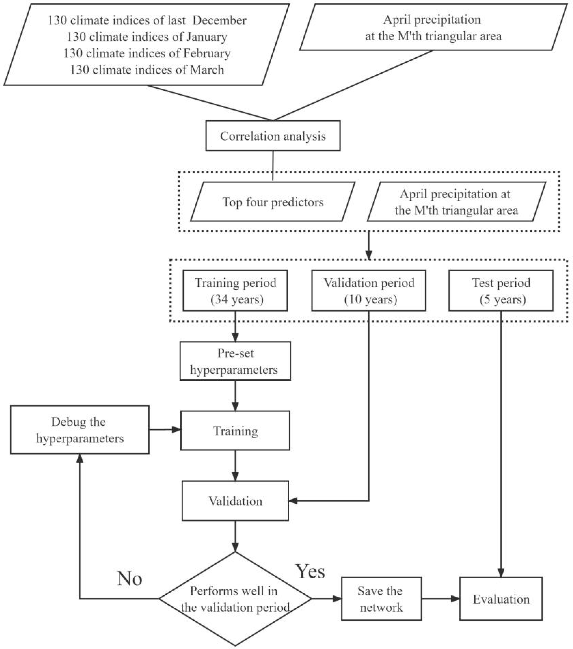
Figure 7 shows the flow chart of the StinBP sub-model (the model over the Mth triangular area), with April precipitation forecasting as an example. The inputs of the BPNN are the series of the top four climate indices most correlated with the triangular area mean precipitation for April, which is, namely, the expected output.

2.3.4. Genetic Algorithm (GA)

The GA is used to optimise the initial weights and biases of BPNN. The initial weights and biases are the starting point for the gradient descent method to find the optimal weights and biases, and the choice of the starting point is crucial to seek the optimal solution in a global optimization problem. The initial weights and biases taken randomly tend to trap the network in a local optimum, which is a widely recognised problem in BPNN training. The GA is able to determine the starting point of the gradient descent method, from which it is possible for the BPNN to converge to the global optimal solution by training. The GA has now been widely used in the field of artificial neural network optimisation [42,43].
For given data, there is an upper limit of the BPNN simulation capability. In the three previous schemes, i.e., SregBP, SstnBP, and StinBP, the aim of hyperparameter optimization is to make the simulation close to the upper limit under a certain scheme. However, the key hyperparameters, i.e., the initial weights and biases, are not involved in debugging. Strictly speaking, there is no assurance that the simulation has reached the upper limit. To confirm this conjecture, only the initial weights and biases are adjusted compared to the StinBP model, while the remaining hyperparameters remain unchanged. The initial weights and biases are optimised using the GA, and the goal of the optimisation is to make the simulation error as low as possible during the validation period, which is unchanged compared to the previous schemes, i.e., SregBP, SstnBP, and StinBP. The improved model is noted as StinGABP.

2.3.5. Evaluation Indices

The indices to evaluate the model in this paper are the mean absolute percentage error (MAPE), the root mean square error (RMSE), the anomaly sign consistency rate (AR), the anomaly correlation coefficient (ACC), and the Ps score, which are conventionally used in meteorological operations. Formulas for MAPE, RMSE, AR, and ACC are shown in Equations (2)–(5) [44].
M A P E i = 1 T t = 1 T P t O t O t × 100 % ,
R M S E i = 1 T t = 1 T P t O t 2 ,
A R t = N 0 N × 100 % ,
A C C t = i = 1 N R f i R ¯ f i R o i R ¯ o i i = 1 N R f i R ¯ f i 2 i = 1 N R o i R ¯ o i 2 ,
where T is the length of the hindcast period (i.e., the test period) by year and N is the number of the stations evaluated, Pt and Ot are the hindcast and observed value of precipitation in the pre-summer rainy season at a station, respectively, N0 is the number of stations at which the hindcast anomaly signs are consistent with the observed anomaly signs in a given year of the hindcast period, Rfi is the hindcast value of the Anomaly percentage of precipitation in a given year of the hindcast period with Roi, which is the observed value correspondingly in that year, and R ¯ f i and R ¯ o i are the mean values of the Rfi and R oi series, respectively. MAPE and RMSE are applied to evaluate the performance of the model over the hindcast period in terms of time scale, while AR and ACC describe the similarity of the spatial patterns of the hindcast and observed precipitation.
Ps score is a conventional evaluation index for monthly and seasonal forecasting models [45]. The unique point is that when precipitation is anomalous, a bonus score is assigned if the model forecasts the anomaly correctly, and when precipitation is extremely anomalous, a penalty is applied if the model fails to forecast the anomaly. The observed precipitation is graded according to the Anomaly percentage (Table 2) [44].
Equation (6) shows the Ps score formula. The detailed meaning of the letters and the steps to calculate the Ps score can be found in the paper of Li et al. [45]. In the formula, a, b, and c are the weights, which are taken as 1, 2, and 1, respectively, in this paper.
P S = 100 × a × N 0 + b × N 1 + c × N 2 N N 0 + a × N 0 + b × N 1 + c × N 2 + M

3. Results

3.1. Comparison of Simulation for Different Schemes

The simulation error of the initial model (i.e., SregBP) and the three improving schemes (i.e., SstnBP, StinBP, and StinGABP) over the training and validation periods are compared in Table 3.
The following information can be seen in Table 3. (1) The overall simulation error for the training and validation periods for each month of the SregBP model is large. (2) The upper limit of the model’s capability to simulate precipitation in the pre-summer rainy season is slightly enhanced by replacing the predictors with climate indices more correlated on the basis of the SregBP model. In May and June, the overall MAPE for the training and validation periods is reduced by about 5%, and the RMSE by about 15 mm. (3) Based on the SstnBP model, the upper limit of the model capability to simulate precipitation is apparently increased by preprocessing the precipitation data. The overall RMSE for the training and validation periods in each month is reduced by more than 15 mm, together with the overall MAPE reduced by more than 40% in April and by more than 15% in May and June. (4) Based on the StinBP model, the initial weights and biases are optimised using GA, and the overall MAPE in each month is reduced slightly while the RMSE increases. The simulation in the validation period is improved at the expense of a worse simulation in the training period. In other words, part of the error is transferred from the validation period to the training period, while the overall error is barely reduced.
Table 3 confirms the previous conjectures, e.g., the predictors more correlated with the precipitation can improve the simulation for every single station, through which the precipitation forecast for the region is improved as a whole. By improving the internal characteristics of the data using the TIN to preprocess precipitation data, the BPNN model substantially improves the simulation performance. Additionally, the GA has the advantage of global optimization compared with the BPNN, which might fall into local optimization and could lead to a better simulation. Surprisingly, in this paper, GA used in BPNN cannot improve the simulation capability of the model in the training and validation periods. The excellent simulation in the validation period may also lead to the problem of overfitting, and the hindcast in the test period is not necessarily as good.
By comparing the simulation and prediction values with the observations, it can be found that MAPE tends to be high when the minimum value is observed. When the maximum observation occurs, the RMSE is easily inflated. The models in this paper are weak to predict the extreme values. TIN improves MAPE and RMSE by smoothing observation data.

3.2. Hindcast and Model Evaluation

In the previous section, two BPNN models (StinBP and StinGABP) with better simulation and equivalent simulation capabilities are identified, and these two models are used in this section to hindcast the precipitation during the pre-summer rainy season in the hindcast period (i.e., the test period, 2013–2017). The model evaluation is divided into two parts: (1) The mean error of hindcasting is compared with its own simulation error in the training and validation periods to assess whether the model is overfitting. (2) The model performance in the hindcast period is compared with that of the FGOALS-f2 model results to evaluate the forecast capability of the model developed in this study.

3.2.1. Judgment of Overfitting

A model is defined to be overfitting if the simulation error is equivalent and low in both the training and validation periods, but the forecast error is significantly higher in the test period [46]. Only if the forecast error already exists can the model be determined to be overfitting.
Table 4 lists the comparison between the simulation error and the hindcast error for different models (i.e., StinBP and StinGABP). The RMSE of the StinBP model in the hindcast period increases in all months compared to the simulation error, rising by 22 mm in April, 41 mm in May, and 11 mm in June, respectively, as does the RMSE of the StinGABP model, rising by 26 mm in April, 102 mm in May, and 94 mm in June, respectively. The increase in StinGABP RMSE during the hindcast period is much higher than that of StinBP RMSE in May and June. The MAPE of the StinBP model in the hindcast period also increases in all months compared to the simulation error, but not greatly, with the mean increase in MAPE turning out to be 11% over the three months. Meanwhile, the mean increase in StinGABP MAPE is 28%, which is 17% higher than that of the StinBP mode.
It can be concluded that both models are overfitting, in which the StinBP model is relatively slight overfitting. In this study, optimising the initial weights and biases of BPNN by GA leads to an increase in the degree of overfitting.

3.2.2. Evaluation of Forecasting Capability

In practical applications, the observed precipitation data based on stations are often processed into the mean values over areas as input items to systems, e.g., runoff models and schemes of programming and management of water resources. The outputs of the StinBP model and StinGABP model are the mean precipitation over triangular areas, which are intended to meet the requirements of practical applications. In order to keep the spatial scale of the model outputs consistent with those of the evaluation indices, the hindcast precipitation is spatially interpolated to obtain the hindcast values at the stations. Similarly, the hindcast precipitation for April, May, and June are summed to obtain the hindcast value for the pre-summer rainy season. The FGOALS-f2 model hindcast data are processed in the same way.
The anomaly sign consistency rate (AR), the anomaly correlation coefficient (ACC), and the Ps score, which are conventionally used in meteorological operations, are calculated for comparison. Table 5 lists the scores of evaluation indices for the StinBP model, the StinGABP model, and the FGOALS-f2 model have a hindcast period of 5 years. Comparing the scores over the hindcast period, the results of the two improved models in this paper are equivalent to that of the FGOALS-f2 model and less stable. The AR and Ps scores of the StinGABP model are higher than the results of the FGOALS-f2 model in 2015–2017, with the maximum difference of AR appearing in 2016 at 11.8% and the maximum difference of Ps score appearing in 2016 at 11.4. The mean scores of the StinGABP model hindcast are higher than the results of the FGOALS-f2 model; the AR is 1.7% higher, the ACC is 0.012 higher, and the Ps score is 1.6 higher. While the mean scores of the StinBP model hindcast are lower than the results of the FGOALS-f2 model, the AR is 0.2% lower, the ACC is 0.033 lower, and the Ps score is 1.3 lower. In terms of AR and Ps scores, the StinGABP model hindcast is substantially better than that of the FGOALS-f2 model in 2015–2017. In terms of mean scores, the StinGABP model hindcast is slightly better than the results of the FGOALS-f2 model. At the same time, the StinBP model is slightly less effective.
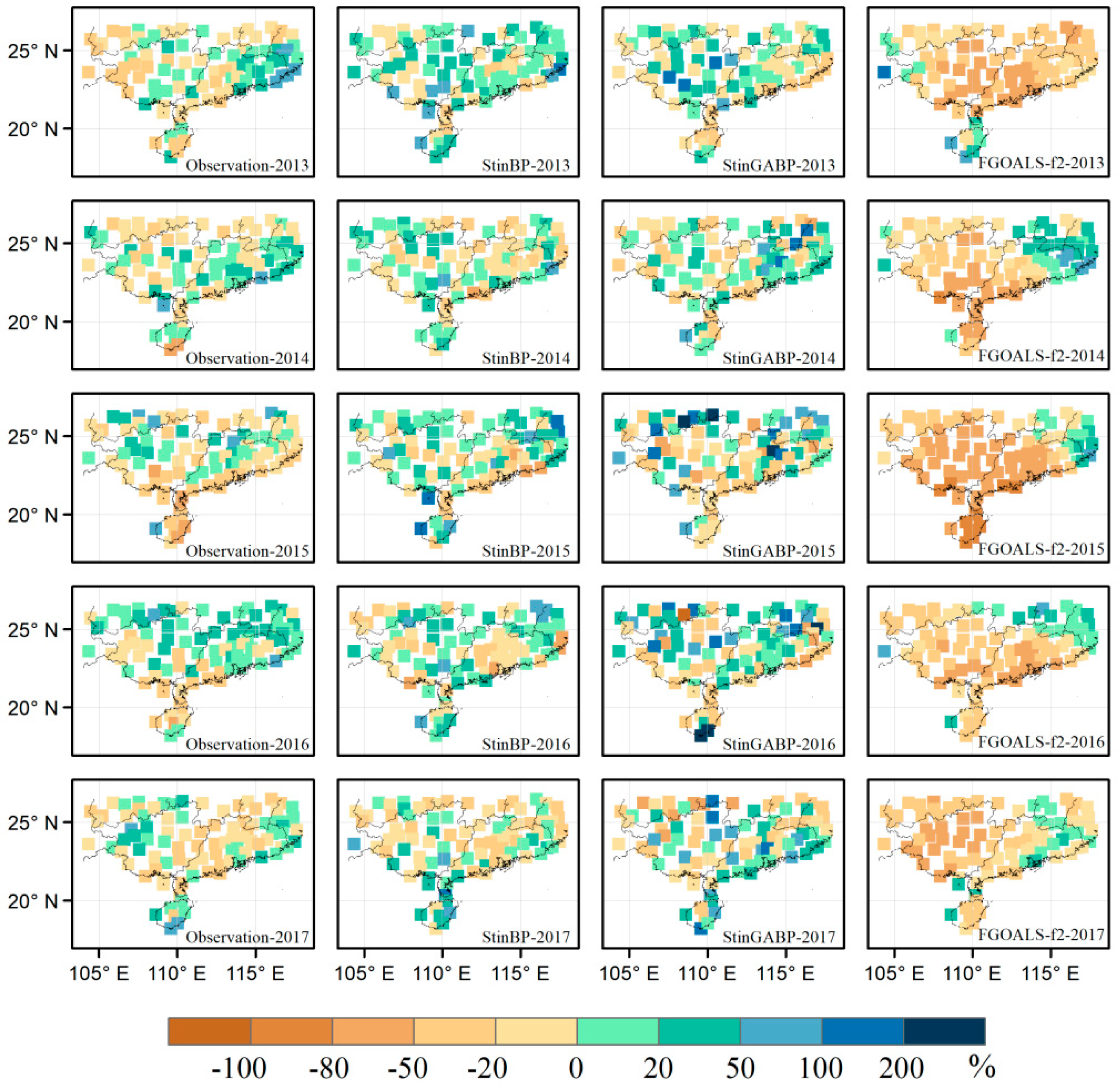
Both the improved models and the FGOALS-f2 model performed poorly in 2013 and well in 2015 and 2016. There is no obvious difference in the grades of total precipitation during the pre-summer rainy season in the three years, so the reason for the different performance of the three models in different years may be the distinctions between the spatial patterns of precipitation. According to Figure 8, the spatial distributions of pre-summer precipitation in 2015 and 2016 are similar, and the centers of the precipitation in 2015 and 2016 are northward compared to 2013. Different forecast methods may be suitable for different spatial patterns of precipitation, so the hindcast scores of the three models in 2015 and 2016 are better than those in 2013. The spatial patterns of pre-summer precipitation are highly correlated to the SST of key regions [47] and the situation of the previous low-level wind field [48]. Therefore, it may be significant for these three models (i.e., StinBP, StinGABP, and FGOALS-f2) to enhance the accuracy of forecasting by taking these two factors into consideration.
Figure 9 shows the spatial distributions of the observed and hindcast values of anomaly percentage of pre-summer precipitation over 2013–2017. Focusing on the high and low centers of the observed precipitation, spatial distributions of the hindcast precipitation of all three models in 2013 differ from the observation. The spatial distribution of the StinGABP model hindcast precipitation in 2014 is the closest to the observation. In 2015, the StinBP model performed well in the coastal region of Guangdong, as did the StinGABP model in Hainan Island. The spatial distribution of the StinGABP model hindcast precipitation in 2016 was similar to the observation, while the StinBP model performed better in 2017.
The hindcasts of the three models over the hindcast period behave differently. The spatial pattern of the StinBP model hindcast precipitation is less spatially varied, with a few extreme values. The spatial variation is large for the StinGABP model hindcast precipitation, with more extreme values in 2015 and 2016. In addition, the spatial distributions of the FGOALS-f2 model hindcast precipitation over the five years present an inter-annual similarity. Therefore, from the perspective of the spatial distribution of precipitation, the hindcasts of the StinBP model and StinGABP model are more reasonable. The StinBP model performance is weaker than that of StinGAPB in predicting extremes because BPNN is enabled to capture few connections between predictors and the extremes through training due to the small sample of extremes. However, the StinGABP model may not be much better at predicting extremes as well. The extreme outputs of the StinGABP model may come from overfitting rather than the physics of precipitation extremes because we did not set a hyperparameter for each station, and the GABP is much more likely to overfit than BP [49,50]. In general, considering the spatial distributions of the hindcast precipitation, the StinGABP model performs better than the StinBP model.

4. Discussion

Although precipitation data in this study are organized at the stations, the gridded precipitation datasets are also applicable for modeling [51]. Actually, the TIN preprocessing of station precipitation data in this work is a special kind of gridding. Zhang et al. [31] used a gridded precipitation dataset and obtained reliable precipitation prediction results, which confirms the effectiveness of the gridded precipitation dataset. Therefore, it is applicable to carry out similar studies in many regions of the globe despite the lack of observational precipitation data.
The models in this study present apparently better forecasts in May and June than in April in general (Table 3 and Table 4). The major reason may be that the type of precipitation in April is different from that in May and June, with frontal rain in April and monsoon rain in May and June mainly [52], suggesting that the dynamical and physical processes in the rainfall events might be quite different over South China and adjacent areas. This is also consistent with the fact that there are also large differences in the climate indices influencing precipitation in these three months, which implies that the forcings by large-scale circulation in different months differ greatly. In addition, it might also be arguable whether the major climate indices influencing precipitation in April have been included in the 130 climate indices in this study, as shown in Supplementary Materials.
The initial precipitation data are locally homogenized after preprocessing and some of the extreme values are lost, which is an inevitable problem coming from regionalization. Keeping the spatial distribution of precipitation unchanged at most, the TIN in this study is the most simplified method of regionalization. In this paper, these extreme values are interference signals that bring the accuracy of the simulation down. However, in actual forecasting, the extreme values are precisely the most important. The focus of subsequent research is to improve the model’s capability to forecast extreme precipitation while keeping the overall error as low as possible.
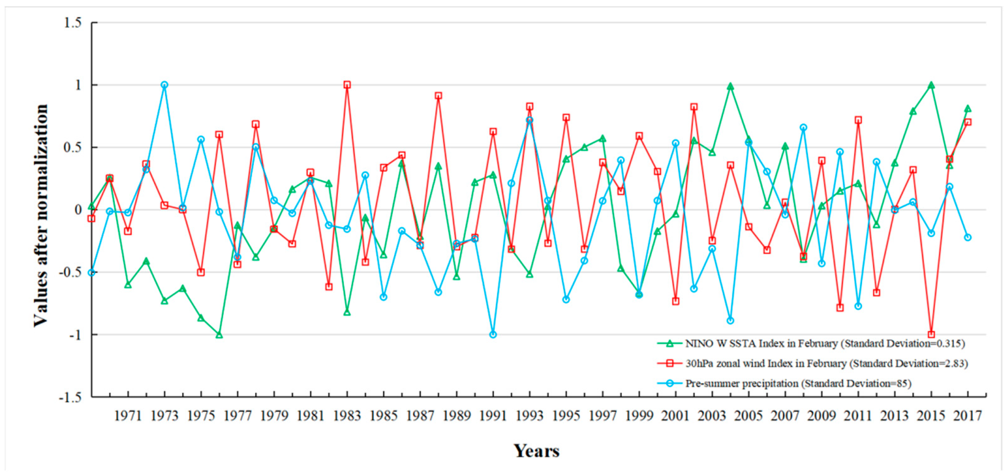
Under the background of global climate change, precipitation in the pre-summer rainy season over South China shows a slightly downward trend. To investigate whether the BPNN is able to capture the trend, a simple experiment has been designed as a feasibility analysis prior to the study above. The total precipitation in the pre-summer rainy season of the entire region is taken as the expected output, and four predictors with high correlations are taken to establish a BPNN. The four predictors are ranked in the descending order of correlations: NINO W SSTA Index in February (the correlation coefficient is −0.361), 30 hPa zonal wind Index in February (the correlation coefficient is −0.355), Pacific Polar Vortex Intensity Index in January, and Tropic Indian Ocean Dipole Index (IOD) in December. The series of the NINO W SSTA Index in February, the Pacific Polar Vortex Intensity Index in January, and the pre-summer precipitation over the 49 years are compared in Figure 10.
Coming with global climate change, long-term transformations appear in the wind, temperature, pressure, and moisture fields, which, in turn, affect precipitation. With global warming, each of these four winter climate indices has the following trends. There is a clear upward trend in the winter NINO W SSTA Index. Zonal winds in the stratosphere have exhibited a long-term east–west oscillation, i.e., the stratospheric quasi-biennial oscillation (QBO), with a weakening trend in the amplitude and a lengthening trend in the wave period [53]. The overall area of the Arctic Polar Vortex has tended to reduce [54]. The eastern surface of the Indian Ocean has been warming slower than the western part. Additionally, the number of years with IOD-positive winter phases is increasing [55]. Anomalies in these four climate indices can bring about anomalies in the pre-summer precipitation. There is a large negative correlation between the winter NINO W SSTA Index and the precipitation [56]. In addition, the precipitation decreases correspondingly in years when the Pacific Polar Vortex weakens [57]; the relatively small area of the Pacific Polar Vortex means that the westerlies are straight and would restrain the Polar Vortex, so it is unfavorable for the cold air to meet the warm and moist air to form precipitation and in years when the South China sea summer monsoon is strengthened during the easterly phase of QBO [58]. Moreover, the positive winter phase of IOD leads to anomalously low precipitation in the pre-summer rainy season [59].
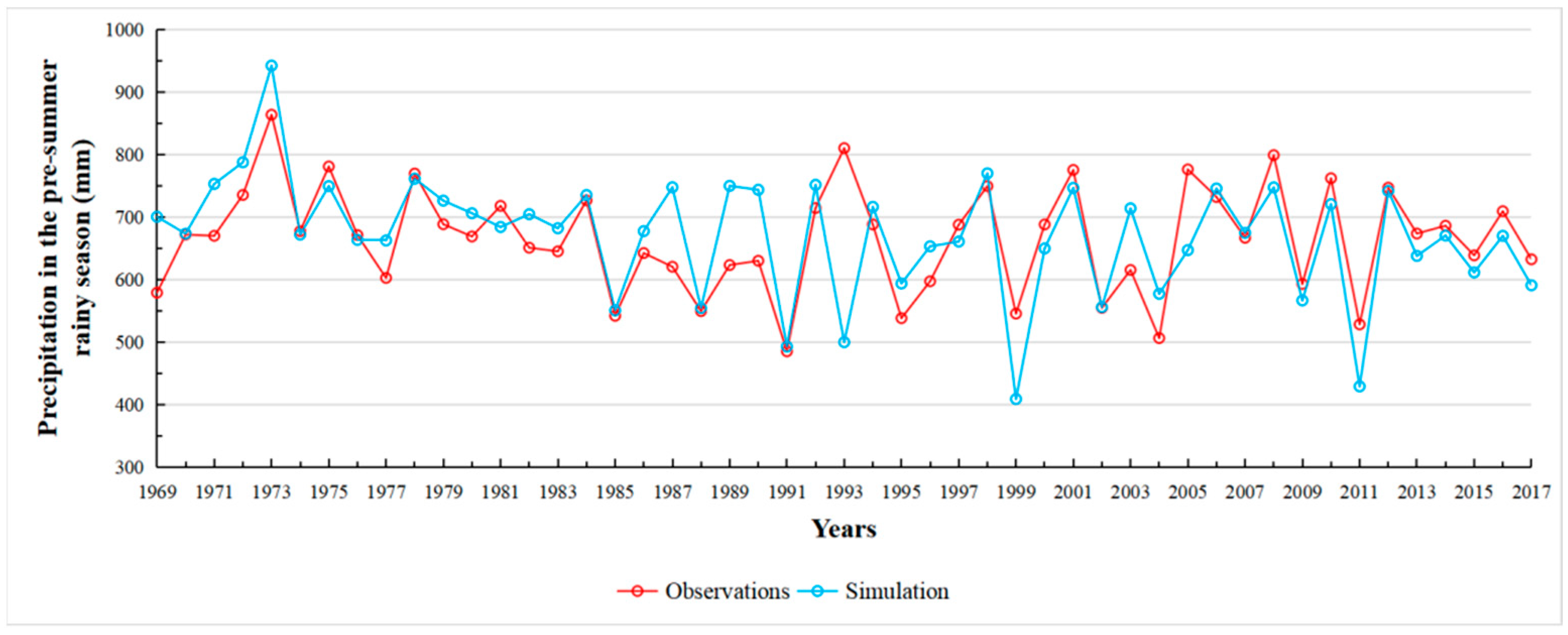
If precipitation simulated by the BPNN above in this section is consistent with the observations in the pre-summer rainy season, it can be inferred that the physics between the predictors and the precipitation, which have been confirmed by the studies, can be learned by BPNN. Figure 11 shows the simulated precipitation series compared to the observed precipitation series. The simulated precipitation series has an overall decreasing trend, trending opposite to the observations in only a few single years. This confirms that the models in this study can combine the physics into the model structure to realize precipitation forecasting, even though some climate indices affecting precipitation in China’s monsoon region shifted abruptly in the 1990s [60], making it more difficult to simulate the land–air and sea–air interactions. It is also in this way that the BPNN captures the trend of decreasing precipitation in the pre-summer rainy season under the background of global climate change.

5. Summary

In this paper, the models based on BPNNs are established for precipitation forecasting during the pre-summer rainy season in South China. The training, validation, and test sets are divided according to the ratio 7:2:1, i.e., over 1969–2002, 2003–2012, and 2013–2017, respectively. Different inputs, different expected outputs, and different schemes for hyperparameter optimization are chosen, respectively, in the four experiments, i.e., SregBP, SstnBP, StinBP, and StinGABP. After training and hyperparameter optimization, the two models performing better (i.e., StinBP and StinGABP) are applied to hindcast the pre-summer precipitation during 2013–2017, and the results are compared with that of the FGOALS-f2 model to evaluate the capability of a forecast for the two models.
In this paper, a TIN is proposed for use in the processing of precipitation data, which changes the internal characteristics of the data and raises the upper limit of the BPNN simulation capability. The internal characteristics of data determine the upper limit, and the simulation approaches the upper limit as closely as possible through hyperparameter optimization. As a new method for preprocessing precipitation data, TIN keeps the spatial distribution of precipitation unchanged at most, i.e., because the TIN in this study is the most simplified method of regionalization using only three locations of the stations, it presents more stable forecasts than those by three separate stations. As a result, TIN gives the hindcasts closer to observations.
BPNN with the initial weights and thresholds optimised by GA in this paper tend to be overfitting. It can be inferred that GA is not applicable to all BPNNs. However, considering the spatial distributions of the hindcast precipitation, the StinGABP model performs better than the StinBP model; considering the mean scores of the hindcasts, the StinBP model is improved by GA.
The MAPE of the improved model hindcasts can be controlled at about 35% and RMSE at about 225 mm. The AR comparing the StinGABP model hindcast with the observation is less than 50% in only one season during the hindcast period, and the highest is 64.5%. The model capability for precipitation forecasting during the pre-summer rainy season is equivalent to that of the FGOALS-f2 model, with the hindcast results turning out to be slightly better, which suggests that even the classical machine learning method (BPNN plus GA) can present better performance than a much more complex dynamical model for precipitation forecast in South China.

Supplementary Materials

The following supporting information can be downloaded at: https://www.mdpi.com/article/10.3390/w16101423/s1.

Author Contributions

Conceptualisation, X.-M.Z., B.-Z.W., and S.-J.L.; methodology, B.-Z.W.; software, B.-Z.W.; validation, B.-Z.W. and S.-J.L.; formal analysis, B.-Z.W. and X.-M.Z.; investigation, B.-Z.W. and X.-M.Z.; resources, S.-J.L., I.U. and X.-M.Z.; data curation, B.L., Z.-X.Z. and J.Z.; writing—original draft preparation, B.-Z.W., X.-M.Z. and S.-J.L.; supervision, X.-M.Z. and B.L.; project administration, B.L., X.-M.Z., J.Z. and I.U.; funding acquisition, B.L., X.-M.Z., J.Z. and I.U. All authors have read and agreed to the published version of the manuscript.

Funding

This research was financially supported by the National Key Research and Development Program of China under Grant Nos. 2021YFA070298 and 2022YFC3202801, the National Natural Science Foundation of China under Grant Nos. 42350410438, and the China Postdoctoral Science Foundation Grant 2023M730928. This work was also partially supported by the National Key Scientific and Technological Infrastructure project “Earth System Numerical Simulation Facility” (EarthLab).

Data Availability Statement

Data will be made available on request.

Conflicts of Interest

The authors declare no conflicts of interest.

References

  1. Ding, Y.H. Monsoons over China; Springer: Dordrecht, The Netherland, 1994; pp. 135–136. [Google Scholar]
  2. Hu, Y.M.; Zhai, P.M.; Luo, X.L.; Lv, J.M.; Qin, Z.N.; Hao, Q.C. Large scale circulation and low frequency signal characteristics for the persistent extreme precipitation in the first rainy season over South China in 2013. Acta Meteorol. Sin. 2014, 72, 465–477. (In Chinese) [Google Scholar]
  3. Zhao, Y.C.; Wang, Y.H. A review of studies on torrential rain during pre-summer flood season in South China since the 1980’s. Torrential Rain Disasters 2009, 28, 3–38. (In Chinese) [Google Scholar]
  4. Lin, A.L.; Ji, Z.P.; Gu, D.J.; Li, C.H.; Zheng, B.; He, C. Application of atmospheric intraseasonal oscillation in precipitation forecast over South China. J. Trop. Meteorol. 2016, 32, 878–889. (In Chinese) [Google Scholar]
  5. Qiang, X.M.; Yang, X.Q. Onset and end of the first rainy season in south China. Chin. J. Geophys. 2008, 51, 1333–1345. (In Chinese) [Google Scholar]
  6. Li, Z.H.; Luo, Y.L.; Du, Y.; Chan, C.L. Statistical characteristics of pre-summer rainfall over South China and associated synoptic conditions. J. Meteorol. Soc. Jpn. Ser. II 2020, 98, 213–233. [Google Scholar] [CrossRef]
  7. Chen, Y.M.; Qian, Y.F. Numerical study of influence of the SSTA in Western Pacific warm pool on precipitation in the first flood period in South China. J. Trop. Meteorol. 2005, 21, 13–23. (In Chinese) [Google Scholar]
  8. Yang, H.; Sun, S.Q. The characteristics of longitudinal movement of the subtropical high in the Western Pacific in the pre-rainy season in South China. Adv. Atmos. Sci. 2005, 22, 392–400. [Google Scholar]
  9. Zhou, X.Y.; Cheng, Z.Q.; Li, H.W.; Hu, D.M. Comparison between the roles of low-level jets in two heavy rainfall events over South China. J. Meteorol. Res. 2022, 36, 326–341. [Google Scholar] [CrossRef]
  10. Hussain, A.; Hussain, I.; Ali, S. Assessment of precipitation extremes and their association with NDVI, monsoon and oceanic indices over Pakistan. Atmos. Res. 2023, 292, 106873. [Google Scholar] [CrossRef]
  11. Wu, H.Q.; Zhang, A.H.; Jiang, B.R.; Qin, W. Relationship between the variation of Antarctic sea ice and the pre-flood season rainfall in South China. J. Nanjing Inst. Meteorol. 1998, 21, 266–273. (In Chinese) [Google Scholar]
  12. Yao, S.X.; Huang, Q.; Zhao, C. Variation characteristics of rainfall in the pre-flood season of South China and its correlation with sea surface temperature of Pacific. Atmosphere 2016, 7, 5. [Google Scholar] [CrossRef]
  13. Cai, X.Z. The influence of abnormal snow cover over Qinghai-Xizang Plateau and East Asian monsoon on early rainy season rainfall over South China. J. Appl. Meteorol. Sci. 2001, 12, 358–367. (In Chinese) [Google Scholar]
  14. Wu, X.S.; Guo, S.L.; Ba, H.H.; He, S.K.; Xiong, F. Long-range precipitation forecasting based on multi-pole sea surface temperature. J. Hydraul. Eng. 2018, 49, 1276–1283. (In Chinese) [Google Scholar]
  15. Singhrattna, N.; Rajagopalan, B.; Clark, M.; Krishna Kumar, K. Seasonal forecasting of Thailand summer monsoon rainfall. Int. J. Climatol. A J. R. Meteorol. Soc. 2005, 25, 649–664. [Google Scholar] [CrossRef]
  16. Zeng, X.M.; Xi, C.L. Study of the effects of reducing systematic errors on monthly regional climate dynamical forecast. J. Trop. Meteorol. 2009, 15, 102–105. [Google Scholar]
  17. Zhao, S.Y.; Yang, S.; Deng, Y.; Li, Q.P. Skills of yearly prediction of the early-season rainfall over southern China by the NCEP climate forecast system. Theor. Appl. Climatol. 2015, 122, 743–754. [Google Scholar] [CrossRef]
  18. Wang, D.H.; Zhao, Y.F. Effective approaches to extending medium-term forecasting of persistent severe precipitation in regional models. Atmos. Ocean. Sci. Lett. 2018, 11, 150–156. [Google Scholar] [CrossRef]
  19. Chen, J.; Pang, B.; Wu, Z.Q.; Chen, F.J.; Chen, Y.X.; Liu, X.; Ma, Y.N. Evaluation of fine-scale precipitation forecast of GRAPES_Meso 3 km convective-scale model in early summer rainy season in South China under complex topographical conditions. Trans. Atmos. Sci. 2022, 45, 99–111. (In Chinese) [Google Scholar]
  20. Xie, J.G.; Qin, B.B.; Wang, J.Y. The application of singular value decomposition analysis in the prediction of seasonal rainfall. Acta Meteorol. Sin. 1997, 117–123. (In Chinese) [Google Scholar] [CrossRef]
  21. Huang, Y.; Jin, L. Prediction model for annually first rainy season precipitation in South China and prediction tests. J. Trop. Meteorol. 2011, 27, 753–757. (In Chinese) [Google Scholar]
  22. Lu, Z.; Guo, Y.; Zhu, J.S.; Kang, N. Seasonal forecast of early summer rainfall at stations in South China using a statistical downscaling model. Weather. Forecast. 2020, 35, 1633–1643. [Google Scholar] [CrossRef]
  23. Liu, Y.; Fan, K.; Wang, H.J. Statistical downscaling prediction of summer precipitation in Southeastern China. Atmos. Ocean. Sci. Lett. 2011, 4, 173–180. [Google Scholar]
  24. Guo, Y.; Li, J.P.; Li, Y. Seasonal forecasting of North China summer rainfall using a statistical downscaling model. J. Appl. Meteorol. Climatol. 2014, 53, 1739–1749. [Google Scholar] [CrossRef]
  25. Li, J.; Cheng, J.H.; Shi, J.Y.; Huang, F. Brief introduction of back propagation (BP) neural network algorithm and its improvement. In Advances in Computer Science and Information Engineering. Advances in Intelligent and Soft Computing; Jin, D., Lin, S., Eds.; Springer: Berlin, Germany, 2012; Volume 169. [Google Scholar]
  26. Danandeh Mehr, A. Seasonal rainfall hindcasting using ensemble multi-stage genetic programming. Theor. Appl. Climatol. 2021, 143, 461–472. [Google Scholar] [CrossRef]
  27. Shang, S.H. System Analysis of Water Resources: Methods and Applications; Tsinghua University Press: Beijing, China, 2006; p. 192. (In Chinese) [Google Scholar]
  28. David, S.; John, A.D. Artificial neural network and long-range precipitation in California. J. Appl. Meteorol. Climatol. 2000, 39, 57–66. [Google Scholar]
  29. Min, J.J.; Sun, J.R.; Liu, H.Z.; Wang, S.G.; Cao, X.Z. An improved BP algorithm and its application to precipitation forecast. J. Appl. Meteorol. Sci. 2010, 21, 55–62. (In Chinese) [Google Scholar]
  30. Moustris, K.P.; Larissi, I.K.; Nastos, P.T.; Paliatsos, A.G. Precipitation forecast using artificial neural networks in specific regions of Greece. Water Resour. Manag. 2011, 25, 1979–1993. [Google Scholar] [CrossRef]
  31. Zhang, Z.C.; Zeng, X.M.; Li, G.; Lu, B.; Xiao, M.Z.; Wang, B.Z. Summer precipitation forecast using an optimized artificial neural network with a genetic algorithm for Yangtze-Huaihe River basin, China. Atmosphere 2022, 13, 929. [Google Scholar] [CrossRef]
  32. Valipour, M.; Khoshkam, H.; Bateni, S.M.; Jun, C. Machine-learning-based short-term forecasting of daily precipitation in different climate regions across the contiguous United States. Expert Syst. Appl. 2024, 238, 121907. [Google Scholar] [CrossRef]
  33. Gupta, B.; Negi, S.S. Image denoising with linear and non-linear filters: A review. Int. J. Comput. Sci. Issues 2013, 10, 149–154. [Google Scholar]
  34. Thomas, R.K.; Kevin, E.T. Modern global climate change. Science 2003, 302, 1719–1723. [Google Scholar]
  35. Zhang, L.R.; Wang, X.Z.; Wang, G.Q.; Liu, J.F.; Li, S.M. Consistency and reliability analysis of hydrological sequence in environment change. J. China Hydrol. 2015, 35, 39–43. (In Chinese) [Google Scholar]
  36. Zhou, T.; Chen, Z.; Zou, L.; Chen, X.; Yu, Y.; Wang, B.; Bao, Q.; Bao, Y.; Cao, J.; He, B.; et al. Development of climate and earth system models in China: Past achievements and new CMIP6 results. J. Meteorol. Res. 2020, 34, 1–19. [Google Scholar] [CrossRef]
  37. Ren, H.L.; Wu, Y.; Bao, Q.; Ma, J.; Liu, C.; Wan, J.; Li, Q.; Wu, X.; Liu, Y.; Tian, B.; et al. The China Multi-Model Ensemble prediction system and its application to flood-season prediction in 2018. J. Meteorol. Res. 2019, 33, 540–552. [Google Scholar] [CrossRef]
  38. Liu, J.T.; Chang, H.B.; Hsu, T.Y.; Ruan, X.Y. Prediction of the flow stress of high-speed steel during hot deformation using a BP artificial neural network. J. Mater. Process. Technol. 2000, 103, 200–205. [Google Scholar] [CrossRef]
  39. Safari, M.J.S.; Arashloo, S.R.; Vaheddoost, B. Multiple kernel fusion: A novel approach for lake water depth modeling. Environ. Res. 2023, 217, 114856. [Google Scholar] [CrossRef]
  40. Tsai, V.J.D. Delaunay triangulations in TIN creation: An overview and a linear-time algorithm. Int. J. Geogr. Inf. Syst. 1993, 7, 501–524. [Google Scholar] [CrossRef]
  41. Pratibha, P.S.; Sumit, S.K. Review on digital elevation model. Int. J. Mod. Eng. Res. 2013, 3, 2412–2418. [Google Scholar]
  42. Ding, S.F.; Su, C.Y.; Yu, J.Z. An optimizing BP neural network algorithm based on genetic algorithm. Artif. Intell. Rev. 2011, 36, 153–162. [Google Scholar] [CrossRef]
  43. Zhu, C.H.; Zhang, J.J.; Liu, Y.; Ma, D.H.; Li, M.F.; Xiang, B. Comparison of GA-BP and PSO-BP neural network models with initial BP model for rainfall-induced landslides risk assessment in regional scale: A case study in Sichuan, China. Nat. Hazards 2020, 100, 173–204. [Google Scholar] [CrossRef]
  44. Chen, G.Y.; Zhao, Z.G. Assessment methods of short range climate prediction and their operational application. J. Appl. Meteorol. Sci. 1998, 9, 178–185. (In Chinese) [Google Scholar]
  45. Li, T.; Chen, J.; Wang, F.; Han, R. A correction algorithm of summer precipitation prediction based on neural network in China. J. Arid. Meteorol. 2022, 40, 308–316. (In Chinese) [Google Scholar]
  46. Thomas, M. Machine Learning; McGraw-Hill Education: New York, NY, USA, 1997. [Google Scholar]
  47. Ma, H.; Chen, Z.H.; Jiang, L.P.; Wang, Q.Q.; Lin, Z.J. SVD analysis between the annually first raining period precipitation in South China and the SST over offshore waters in China. J. Trop. Meteorol. 2009, 25, 241–245. (In Chinese) [Google Scholar]
  48. Hu, Y.H.; Rong, Y.S.; Wei, J.; Li, C.H.; Tang, H.B.; Li, S.S. Relationship between pre-flood season precipitation in South China and Indian Ocean SST at earlier stages. Water Resour. Prot. 2017, 33, 106–116. (In Chinese) [Google Scholar]
  49. Chen, Z.; Zhou, L.; Yang, X.; Wang, Z.; Ding, Z. A GABP based method to improved software defect prediction. In Proceedings of the 12th International Conference on Quality, Reliability, Risk, Maintenance, and Safety Engineering (QR2MSE 2022), Emeishan, China, 27–30 July 2022; Volume 2022, pp. 1556–1563. [Google Scholar]
  50. Zhao, M.; Zhang, C.; Weng, Y. Improved artificial neural networks (ANNs) for predicting the gas separation performance of polyimides. J. Membr. Sci. 2023, 681, 121765. [Google Scholar] [CrossRef]
  51. Araghi, A.; Jaghargh, M.R.; Maghrebi, M.; Martinez, C.J.; Fraisse, C.W.; Olesen, J.E.; Hoogenboom, G. Investigation of satellite-related precipitation products for modeling of rainfed wheat production systems. Agric. Water Manag. 2021, 258, 107222. [Google Scholar] [CrossRef]
  52. Zheng, B.; Gu, D.J.; Li, C.H.; Lin, A.L.; Liang, J.Y. Frontal rain and summer monsoon rain during pre-rainy season in South China. Part II: Spatial patterns. Chin. J. Atmos. Sci. 2007, 31, 495–504. (In Chinese) [Google Scholar]
  53. Kawatani, Y.; Hamilton, K. Weakened stratospheric quasibiennial oscillation driven by increased tropical mean upwelling. Nature 2013, 497, 478–481. [Google Scholar] [CrossRef] [PubMed]
  54. Gu, S.N.; Yang, X.Q. Variability of the northern circumpolar vortex and its association with climate anomaly in China. Sci. Meteorol. Sin. 2006, 26, 135–142. (In Chinese) [Google Scholar]
  55. Luo, Y.Y.; Lu, J.; Liu, F.K.; Wan, X.Q. The positive Indian Ocean Dipole-like response in the tropical Indian Ocean to global warming. Adv. Atmos. Sci. 2016, 33, 476–488. [Google Scholar] [CrossRef]
  56. Jia, X.J.; Zhang, C.; Wu, R.G.; Qian, Q.F. Changes in the relationship between spring precipitation in southern China and tropical Pacific-South Indian Ocean SST. J. Clim. 2021, 34, 6267–6279. [Google Scholar] [CrossRef]
  57. Zhang, H.D.; Gao, S.T.; Zhang, Y.S. The interdecadal variation of north polar vortex and its relationships with spring precipitation in China. Clim. Environ. Res. 2006, 11, 593–604. (In Chinese) [Google Scholar]
  58. Zheng, B.; Gu, D.; Lin, A.; Li, C. Dynamical mechanism of the stratospheric quasi-biennial oscillation impact on the South China Sea Summer Monsoon. Sci. China Ser. D Earth Sci. 2007, 50, 1424–1432. [Google Scholar] [CrossRef]
  59. Li, C.X.; Zhao, T.B. Seasonal responses of precipitation in china to El Niño and positive Indian Ocean Dipole modes. Atmosphere 2019, 10, 372. [Google Scholar] [CrossRef]
  60. Gao, T.; Wang, H.J.; Zhou, T.J. Changes of extreme precipitation and nonlinear influence of climate variables over monsoon region in China. Atmos. Res. 2017, 197, 379–389. [Google Scholar] [CrossRef]
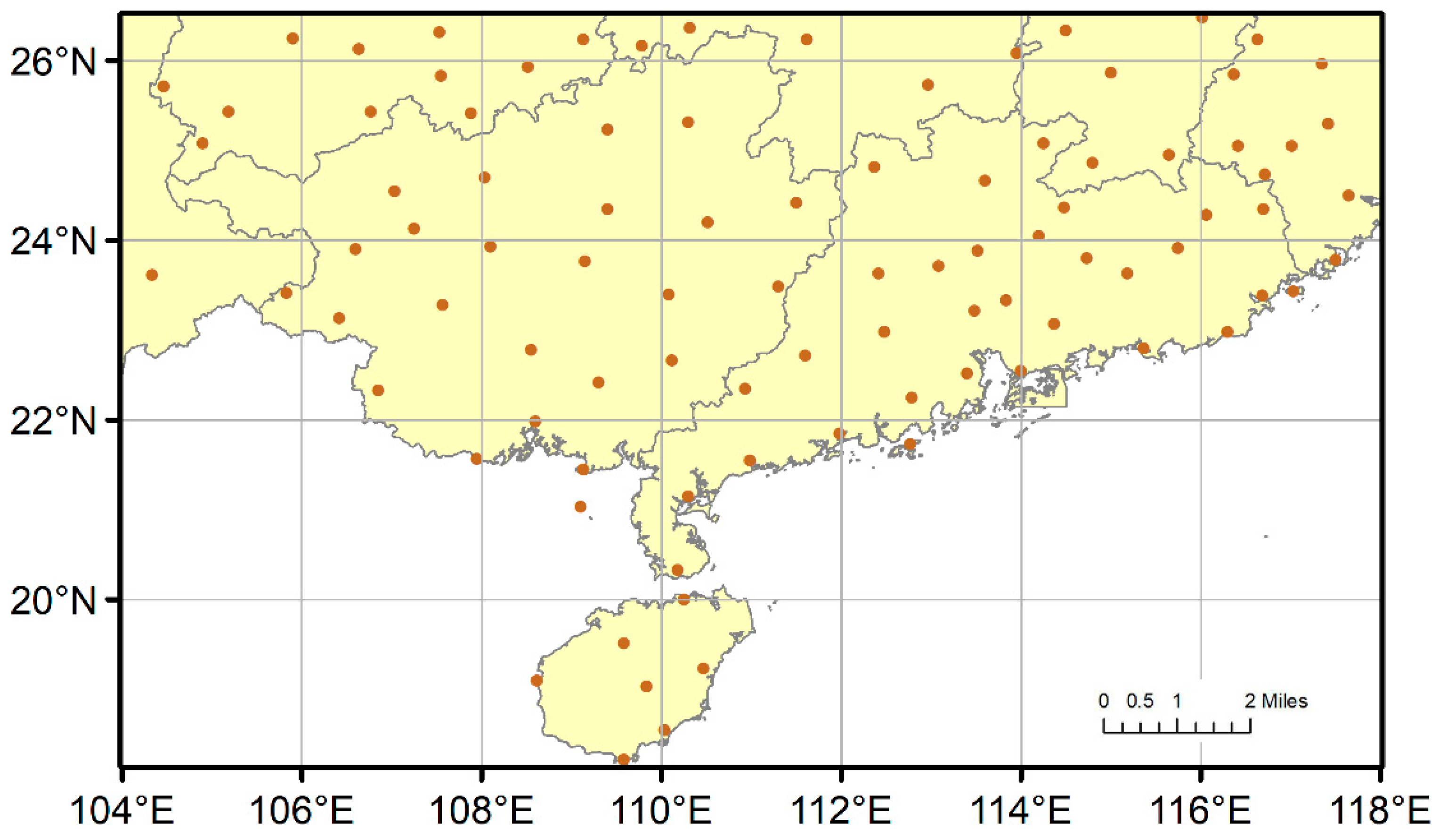
Figure 1. Locations of 93 stations in South China.
Water 16 01423 g001
Figure 2. Structure of a conventional BPNN with one hidden layer.
Water 16 01423 g002
Figure 3. Flow chart of the SregBP sub-model.
Water 16 01423 g003
Figure 4. Flow chart of the SstnBP sub-model.
Water 16 01423 g004
Figure 5. The triangular irregular network (TIN) over South China.
Water 16 01423 g005
Figure 6. Spatial distributions of the annual average precipitation over the multiyears during the pre-summer rainy season before (a) and after (b) preprocessing.
Water 16 01423 g006
Figure 7. Flow chart of the StinBP sub-model with April precipitation forecasting as an example.
Water 16 01423 g007
Figure 8. Spatial distributions of the pre-summer precipitation over the hindcast period. (a) 2013; (b) 2014; (c) 2015; (d) 2016; (e) 2017.
Water 16 01423 g008
Figure 9. Anomaly percentage of precipitation from observations and the models.
Water 16 01423 g009
Figure 10. NINO W SSTA Index in February, Pacific Polar Vortex Intensity Index in January, and pre-summer precipitation during 1969–2017.
Water 16 01423 g010
Figure 11. Observation and simulation series of the pre-summer precipitation during 1969–2017.
Water 16 01423 g011
Table 1. Designed schemes with the training, validation, and test periods over April–June of 1969–2002, 2003–2012, and 2013–2017 respectively.
SchemesInputsExpected OutputInitial Weights
and Biases
Other HyperparametersTraining PeriodValidation PeriodTest Period
SregBPPredictors correlated with the regional precipitationStation precipitationRandomManual debugging1969–20022003–20122013–2017
SstnBPPredictors correlated with the station precipitationAs in SregBPAs in SregBPAs in SregBPAs in SregBPAs in SregBPAs in SregBP
StinBPAs in SstnBPTIN precipitationAs in SregBPAs in SregBPAs in SregBPAs in SregBPAs in SregBP
StinGABPAs in SstnBPAs in StinBPGA optimizationAs in SregBPAs in SregBPAs in SregBPAs in SregBP
Table 2. Grades of precipitation anomalies.
Grades of Precipitation AnomaliesBasis
Extreme R o i 100 %
First grade 50 % R o i < 100 %
Second grade 20 % R o i < 50 %
Normal R o i < 20 %
Table 3. Simulation for different BPNN models.
MonthsModeling
Schemes
Training PeriodValidation PeriodTraining and
Validation Periods
RMSE (mm)MAPE (%)RMSE (mm)MAPE (%)RMSE (mm)MAPE (%)
AprilSregBP77.996.2118.7152.990.2109.1
SstnBP80.899.6110.1133.390.3107.2
StinBP69.257.993.786.075.264.3
StinGABP121.761.761.747.5111.058.5
MaySregBP116.852.5144.374.9125.257.6
SstnBP103.147.4131.374.6111.953.6
StinBP89.332.4112.146.395.035.6
StinGABP130.334.158.022.7117.931.5
JuneSregBP128.453.7183.966.8144.756.7
SstnBP108.746.2170.467.4127.851.1
StinBP95.633.9149.443.1110.136.0
StinGABP157.336.9108.631.5147.735.7
Table 4. Simulation error and hindcast error for StinBP and StinGABP.
MonthsSchemesTraining and
Validation Periods
Hindcast Period
RMSE (mm)MAPE (%)RMSE (mm)MAPE (%)
AprilStinBP75.2 64.3 97.5 78.9
StinGABP111.0 58.5 137.0 87.9
MayStinBP95.0 35.6 136.2 44.4
StinGABP117.9 31.5 220.2 55.1
JuneStinBP110.1 36.0 120.9 46.4
StinGABP147.7 35.7 241.5 66.8
Table 5. Scores of evaluation indices for different models in the hindcast period.
YearsAR(%)ACCPs
StinBPStinGABPFGOALS-f2StinBPStinGABPFGOALS-f2StinBPStinGABPFGOALS-f2
201339.8 38.7 47.3 −0.050 −0.205 −0.169 43.4 40.6 50.0
201463.4 53.8 54.8 0.172 0.134 0.205 64.9 57.0 57.1
201555.9 60.2 55.9 0.097 0.199 0.124 60.2 66.1 61.0
201654.8 64.5 52.7 0.028 0.076 0.250 57.6 68.3 56.9
201749.5 55.9 53.8 −0.027 0.243 −0.026 52.5 61.0 59.8
Mean52.7 54.6 52.9 0.0440.089 0.077 55.758.6 57.0
Disclaimer/Publisher’s Note: The statements, opinions and data contained in all publications are solely those of the individual author(s) and contributor(s) and not of MDPI and/or the editor(s). MDPI and/or the editor(s) disclaim responsibility for any injury to people or property resulting from any ideas, methods, instructions or products referred to in the content.