Abstract
Water majorly contributes to soil erosion. Considering Japan’s humid and rainy climate, severe soil erosion challenges persist even though forests are the country’s dominant land type. Although numerous studies have emphasized the impact of factors such as land use, soil type, and slope steepness on sediment yield, the synergetic effects of slope gradient with varying land cover and soil types are underexplored. Herein, we used the Soil and Water Assessment Tool (SWAT) on a steep catchment to identify high sediment yield areas—as well as factors influencing high sediment yield—and evaluate the effect of slope gradient on the sediment yield of different land cover and soil types. The findings reveal an average annual sediment yield of 0.55 tons ha−1 yr−1 in the Takahashi catchment, with yields tripling in some western subbasins under heavy rainfall. Furthermore, the slope gradient effect is most considerable in bare land, agriculture, and rice land cover, with the average sediment yield of bare land resulting in 2.2 tons ha−1 yr−1 at slope > 45%. Meanwhile, deciduous forests on steep slopes exhibit extreme sediment yield, peaking at 7.2 tons ha−1 yr−1 at slope > 45%. The regosol soil type has one of the highest sediment yield variations in all soil types due to slope gradient.
1. Introduction
Scouring due to precipitation is the primary cause of soil erosion [1]. Soil is a fragile and nonrenewable resource owing to its differing rates of formation from natural geological processes and possible deterioration [2]. The present soil erosion rates are higher in magnitude than soil formation, and this has been a major threat to food security and the sustainability of ecosystems [3]. Soil erosion is a major threat to the global water environment.
Forested catchments play a vital role in high-quality water supplies and provide slope stability and erosion control worldwide [4,5,6]. Forest soil erosion caused by rainwater results in the loss of soil and its organic carbon and nutrients, further damaging the forest ecosystem [7,8]. Moreover, because forested areas exist in regions with high precipitation [9,10], this may further exacerbate the damage to ecosystems, especially concerning climate change [11].
The study of slope effects on soil detachment and sediment yield has frequently been investigated using field sample plots and indoor experimental studies [12,13]. Usually, sediment yield increases congruently with the slope and rainfall intensity. However, the actual interaction of rainfall and slope on sediment yield depends on the soil type and its properties [13].
To plan and develop effective soil conservation measures, identification of areas at risk of soil erosion is a prerequisite. Modeling offers a quantitative and consistent method for estimating soil erosion and sediment output in various contexts [14]. Numerous soil erosion and sediment yield models have been applied to catchments of various conditions and characteristics [15,16,17]. Furthermore, several modeling approaches to slope gradient effects on sediment yield in cultivated land consider different land management practices [15,17].
The Soil and Water Assessment Tool (SWAT) can be used to identify and predict which land is susceptible to erosion, to implement suitable management practices, especially for assessing the effect of precipitation on material transport [18,19,20,21]. SWAT is occasionally used to simulate streamflow and suspended sediment in small, forested catchments, mostly less than 100 km2, for different temporal scales [22,23,24]. SWAT is applied to large continental scales by incorporating agricultural management and point sources and nonpoint sources to examine the water and material cycle and show the spatial and temporal differences in water availability [25,26]. Many SWAT studies have evaluated sediment yield variations based on land use and cover, as well as the slope effects [19,27,28,29]. However, an investigation of the latter that also considers land cover and soil type remains a research gap. Therefore, we explored the relationship between sediment yield and slope gradient for different land cover and soil types based on the SWAT model.
Compared with other countries, Japan’s topography, geology, and fast-flowing rivers, coupled with a rainy climate, result in high sediment transport. Torrential rainfall in July 2018 caused severe water-related disasters, particularly in the Hiroshima and Okayama river basins [30,31,32,33,34,35,36]. This study identified the critical areas for sediment yield in the steep forested catchment, investigated the main factors that influence high sediment yield, and evaluated the slope gradient effect on sediment yield of different land cover and soil types.
2. Materials and Methods
2.1. Study Area
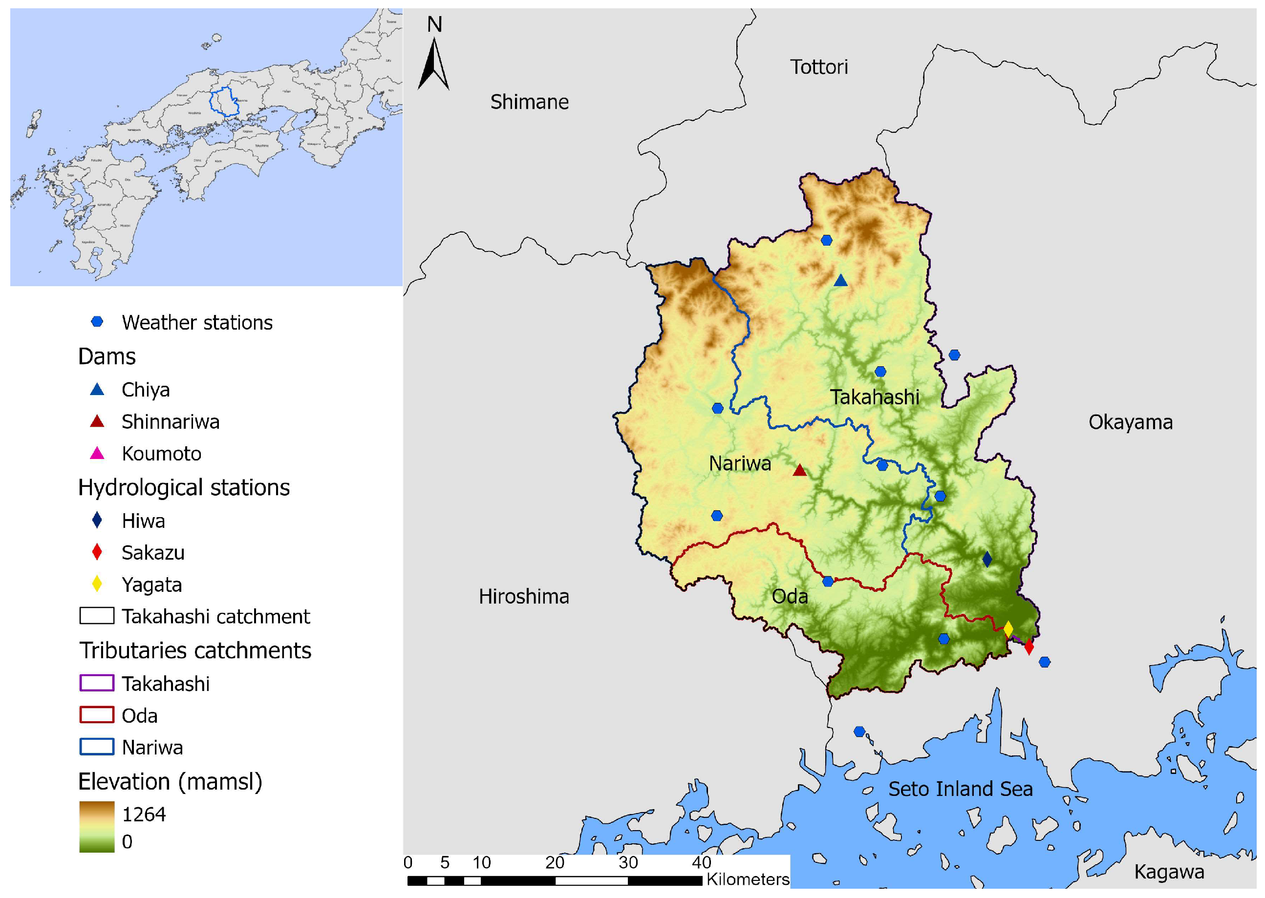
The Takahashi River catchment, with an area of 2670 km2, is located in the Okayama Prefecture of Western Japan (Figure 1). The main river’s total length is 111 km. The major tributaries of the Takahashi River are the Takahashi, Nariwa, and Oda Rivers. The catchment elevation ranges from 0 to 1264 m above sea level. Takahashi River originates from the forested steep slopes of mountainous areas and finally enters the Seto Inland Sea at Kurashiki City.

Figure 1.
Dams and hydrological stations in the Takahashi river system.
The Takahashi catchment is a forested catchment with 84% forest cover, which is 43.74% deciduous forest and 41.05% evergreen (Figure S1). As the hydrological processes of different types of forests differ significantly, the study area had to be divided according to land use in various stages of modeling work [37]. The catchment’s mean slope is 30% and is characterized by a steep slope of greater than 15% occupying 79.15% of the catchment area. The dominant soil type is cambisols, representing 67.25% of the catchment area (Figure S2). The other soil types are regosols (12.06%), andosols (10.52%), gleysols (8.83%), acrisols (1%), and leptosols (0.23%). The andosol and most of the cambisol soil areas are found in the Takahashi and Nariwa tributaries, whereas the Oda tributary mainly comprises gleysols and regosols. The mean annual precipitation across the catchment from 1990 to 2022 was 1328 mm. The geological setting of the Takahashi catchment is 58.3% igneous rock, 36.5% sedimentary rock, and 5.2% metamorphic rock. Based on Ministry of Land, Infrastructure, Transport and Tourism (MLIT) classification, the Takahashi catchment’s geology has 13 subcategories, with granite and rhyolite comprising 44% of the catchment area (Figure 2). The studied catchment has limestone areas, mainly in parts of the Takahashi and Nariwa tributaries.
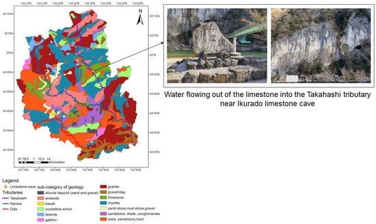
Figure 2.
Outcrop geology of Takahashi catchment showing water flowing out of limestone into the Takahashi tributary.
The studied catchment experienced a devastating flood disaster in 2018 due to a great amount of cumulative precipitation over 48 h (262 mm) rather than the rainfall intensity per hour [34]. Shakti et al. [33] have proved that the Rainfall–Runoff–Inundation (RRI) model is suitable for evaluating the flood inundation analysis of flood-prone river basins, including the Oda tributary of the Takahashi River system. Meanwhile, Nihei et al. [32] have compared the flooding situation of the Oda River in Okayama Prefecture in 2018 and the Kinugawa River in the Ibaraki Prefecture in 2015. Although the Kinugawa River’s inundation area was four times that of the Oda River, the inundation volume was similar because the inundation depth of the Oda River was 5.38 m, which was greater than that of the Kinugawa River at 3.01 m. Along with heavy rainfall and flooding, major rivers in the Okayama Prefecture experienced high sediment transport [34].
2.2. SWAT Model Description
SWAT is a semi-distributed, continuous time-scale model developed by the United States Department of Agriculture (USDA) Agricultural Research Service. The model is used for assessing the impacts of land management practices on hydrological components and water quality and has been successfully applied at scales ranging from small to continental. It is widely used in large, complex watersheds to simulate long-term impacts therein [38]. SWAT requires topography, soil property, land use, and meteorological data—such as precipitation, maximum and minimum air temperature, relative humidity, wind speed, and solar radiation—as input data for the simulation of hydrological components at different time steps. SWAT detaches catchments into subbasins. Subbasins are then dissociated into hydrological response units (HRUs). An HRU is a unit formed by homogeneous land use, soil, and topography [39].
SWAT divides the hydrological cycle into a land phase and a routing phase. The land phase computes the hydrological balance and sediment yields on a daily scale. The land phase of the hydrologic cycle of the SWAT model is based on the water balance equation described in Equation (1):
where is the final soil water content (mm), is the initial soil water content (mm), stands for time (days), is the amount of precipitation on day i (mm), is the amount of surface runoff on day i (mm), is the amount of percolation and bypass flow exiting the soil profile bottom on day i (mm), and is the amount of return flow on day i (mm).
SWAT has two options for rainfall–runoff interaction: the SCS curve number method developed by USDA, and the Green and Ampt Mein–Larson (GAML) method. The SCS curve number method is used for simulating runoff in daily time steps, whereas GAML is used for sub-daily time steps.
The sediment yield was calculated using the Modified Universal Soil Loss Equation, as shown in Equation (2) [40]:
where sed is the sediment yield, is the surface runoff, is the peak discharge, is the HRU area, is the soil erodibility factor, is the cover management factor, is the support practice factor, is the topographic factor, and is the coarse fragment factor. The specific equations for Equation (2) are described in detail in the SWAT model theoretical documentation [39].
2.3. SWAT Model Implementation
In this study, SWAT 2012 (Rev. 685) along with a QGIS interface simulated the daily streamflow and sediment load from 2002 to 2007. The basic data input for topography was derived from the National Aeronautics and Space Administration’s 30 m Shutter Radar Topography Mission Digital Elevation Model (DEM). DEM was used to delineate the stream network and the catchment and derive the slope of the terrain. High-resolution with 10 m land use data for 2006 from the Japan Aerospace Exploration Agency were used for land use input. Soil data were obtained from MLIT. The daily meteorological data from 11 weather stations (11 stations for precipitation, 6 stations for temperature, relative humidity, solar radiation, and wind speed) surrounding the catchment obtained from the Japan Meteorological Agency and the National Agriculture and Food Research Organization were input into the model. Moreover, water management policies in watersheds, including reservoirs, are important for model accuracy [41]. Although several reservoirs stand on the branches of the Takahashi and Nariwa tributaries, the Chiya (2.62 107 m3) and Koumoto (1.11 107 m3) reservoirs on the upstream of the Takahashi tributary and the Shin-nariwa reservoir (8.05 107 m3) on the Nariwa tributary were considered because of their locations, water storage capacity, and data availability.
The study area was divided into 27 subbasins and 2689 HRUs. In creating HRUs, four slope bands were set (<15%, 15–30%, 30–45%, and >45%). The model had a three-year warm-up period, and the simulated model was calibrated from 2002 to 2004 and validated from 2005 to 2007. The model simulation years could be categorized into dry years (2002, 2005, and 2007) and wet years (2003, 2004, and 2006) based on the long-term mean precipitation data. Leta et al. [42] have suggested that, in catchments with large spatial variations of soils, land uses, and geology, which consequently have spatial differences in streamflow-generating processes, simultaneous multisite calibration is preferable. Because Takahashi is a catchment with high spatial heterogeneities, the daily observed streamflow data from three hydrological stations (Sakazu, Yagata, and Hiwa) and daily observed sediment data from the Sakazu station were used for calibration and validation, as Yagata and Hiwa stations do not have the observed sediment data. The streamflow observed data were acquired from MLIT, and the sediment data were obtained from the Okayama River Management Office. Potential evapotranspiration was applied using the Penman–Monteith method, and stream channel sediment routing was performed using the simplified Bagnold equation in this study. The model was calibrated and validated using the auto calibration SWAT-CUP SPE program considering the sensible water balance components of the catchment and the observed data.
2.4. Assessment of Model Accuracy
The coefficient of determination () and Nash–Sutcliffe efficiency (NSE) are widely used statistical indexes for assessing the accuracy of model simulations [19,29,43,44,45,46,47,48]. shows the coefficient of linear correlation between observed and simulated data and ranges from 0 to 1. If its value is closer to 1, the simulated data have good agreement with the observed data. Meanwhile, NSE is a normalized statistic that assesses the relative amount of residual variance in comparison with the measured data variance. NSE can take measurement uncertainty into account and is good for use with continuous long-term simulations and can be used to assess how well a model simulates trends for the output response of concern. Furthermore, percent bias (PBIAS) is used to determine the average model simulation bias. Positive PBIAS values indicate underestimation, whereas negative values indicate overestimation. PBIAS is recommended for use with other statistical indicators to determine a model’s performance [49]. The equations for , NSE, and PBIAS are expressed in Equations (3)–(5), respectively:
where represents the observed data, represents the simulated data, is the mean of the observed data, and is the mean of the simulated data.
2.5. Identifying the Principal Factor for Sediment Yield and Slope Gradient Effects
We conducted principal component analysis (PCA) on sediment yield at the HRU scale to understand the correlations between different components and identify the factors that influence sediment yield. In PCA, we considered land attribute variables related to soil erosion, including topography, soil, and land use. The components analyzed include CN (daily average curve number), Slope (slope percentage rise of HRUs), USLE_K (soil erodibility factor), Sol_AWC (available water capacity of the soil layer), Sol_BD (soil moist bulk density), Sol_K (saturated hydraulic conductivity of soil) and SYLD (sediment yield).
To evaluate slope gradient effects, sediment yields from the HRU outputs were categorized based on land cover and soil type. Next, for each land cover and soil type, sediment yield was classified into four slope gradients (0–15%, 15–30%, 30–45%, and >45%). The leptosol soil type—which represents only 0.23% of the studied catchment—was omitted when considering the relation of soil types and slope gradient on sediment yield variations owing to its limited number of HRU sediment yield results.
3. Results
3.1. Parameterization and Model Performance Assessment
According to the literature and calibration manual, eleven parameters for streamflow and seven parameters for sediment were selected for calibration, as shown in Table S1 [25,38,50]. During the calibration stage, Manning’s “n” roughness of the main channel (CH_N2) and threshold depth of water in the shallow aquifer required for the return flow to occur (GWQMN) variably depending on the tributary, and the SCS runoff curve number (CN2) and soil evaporation compensation factor (ESCO) showed variations between different types of land cover. Groundwater flow from the shallow aquifer to the river occurred when the GWQMN values were lower than or equal to the water depth in the shallow aquifer. The Takahashi and Nariwa tributaries were limestone-influenced areas. According to the observed data from Hiwa station, the model was calibrated to have an increased shallow aquifer flowing into the Takahashi and Nariwa tributaries by setting a low GWQMN value of 200. The Oda tributary and subbasins 22 and 23, which are close to the outlet of the Takahashi River into the Seto Inland Sea, showed the highest GWQMN values (2000 and 3000, respectively). Wang et al. [51] have stated that the karst structures in limestone areas have great permeability and make underground runoff more prevalent than surface runoff. Consequently, the water cycle in limestone environments differs from that in non-limestone areas.
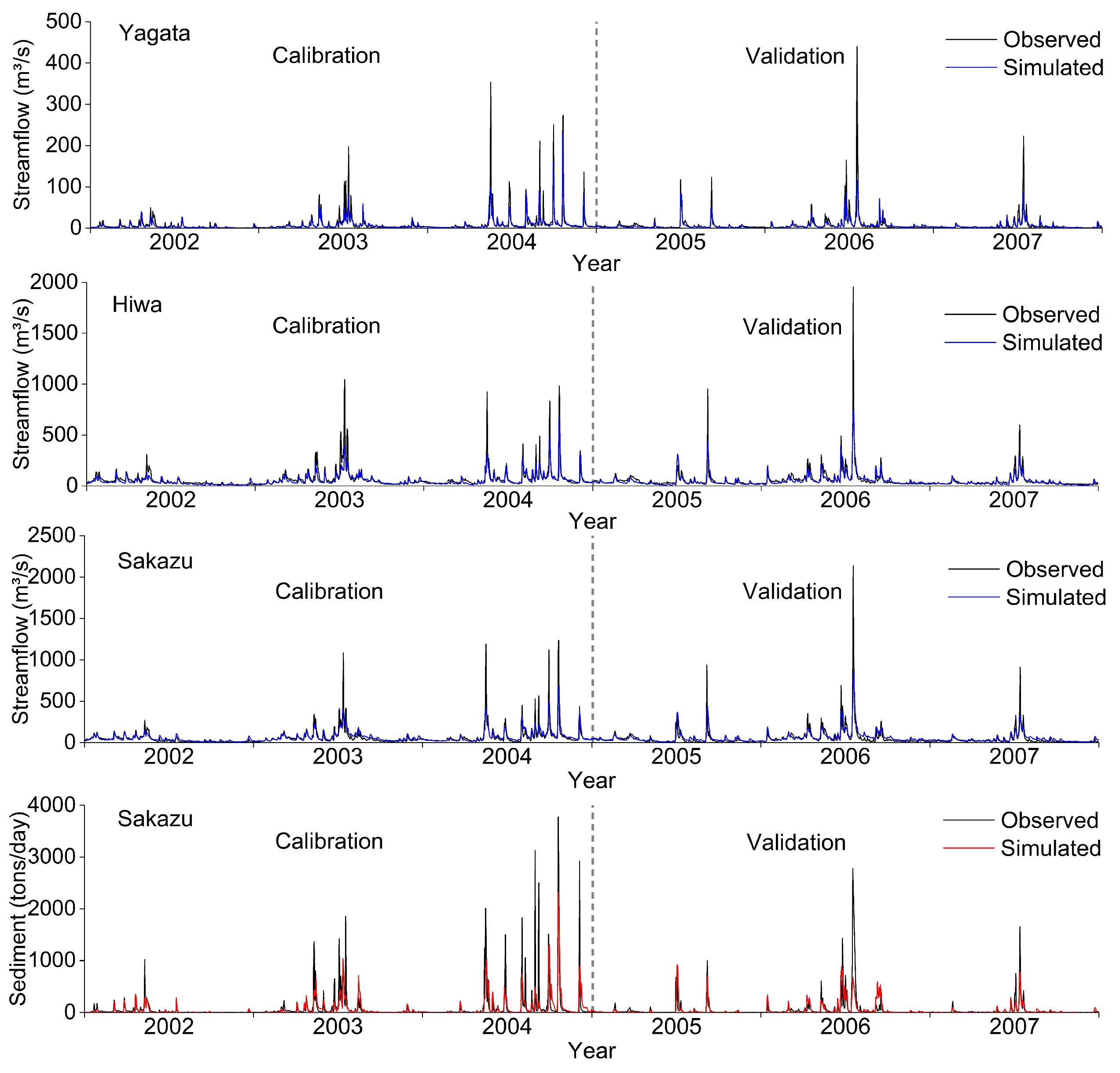
The statistical indexes for the model calibration and validation years as shown in Table 1 were satisfactory according to Moriasi et al. [49]. The NSE values of streamflow calibration were 0.61, 0.68, and 0.7 while validation values were 0.56, 0.7, and 0.65 for the Yagata, Hiwa, and Sakazu stations, respectively. Sediment calibration and NSE validation values at Sakazu station were 0.49 and 0.46, respectively. According to the PBIAS values, the model underestimated the streamflow of Yagata and Hiwa and overestimated that for Sakazu. The sediment PBIAS showed that the model underestimated the sediment yield for the calibration years, and overestimated it for the validation years. Figure 3 shows the goodness of fit between the observed and simulated streamflow and sediment yield. The year 2004 had a unique precipitation period among all the simulated years. Generally, the studied area receives heavy rain in summer, when typhoons occur. However, 2004 had a prolonged rainy period, which ran from the end of spring to early autumn. The model underestimated the sediment in calibration years, which could be due to the prolonged rainy period. Some of the peaks in the figure did not completely match. This part of the flow can be considered as the water discharged into the river through the drainage system during the period. As the drainage system usually responds very quickly, this leads to a higher peak value [52]. Overall, the results of the model are credible.

Table 1.
Statistical performance of the SWAT model for calibration (2002–2004) and validation (2005–2007).
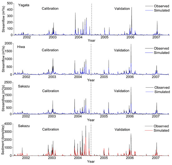
Figure 3.
Calibrated and simulated streamflow and sediment.
3.2. Annual Variations in Sediment Output
Figure 4 shows sediment output variations by subbasin. Among the 27 subbasins, 10 exhibited slight changes in sediment output over the years, and 17 (particularly subbasins 20, 21, 22, and 27) showed pronounced fluctuations. Although subbasins 16 and 18 showed a high sediment output throughout the years, subbasins 20, 21, 22, and 27 showed the highest sediment output in wet years. The subbasins with consistently low sediment output are located in the Takahashi tributary headwater regions, whereas those with the highest fluctuations are located in the Nariwa tributary.
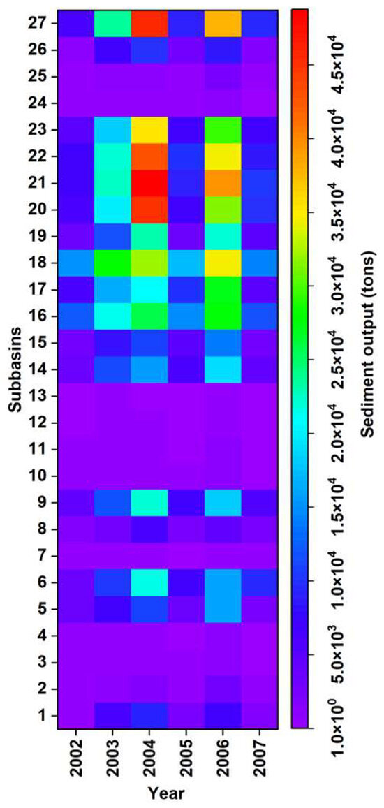
Figure 4.
Annual sediment output variations across subbasins.
The annual average observed sediment output was 19,518.6 tons yr−1, while the simulated value was 17,974.5 tons yr−1, reflecting an 8% underestimation by the model. However, the observed and modeled sediment outputs were comparable regardless of this difference. The sediment load showed a high correlation with total precipitation and the precipitation pattern and intensity. Sediment transport peaked between late spring and mid-autumn (May–September). Among the wet years, 2004 was unique with a prolonged rainy period (Figure S3), having the highest sediment output (38,705.5 tons) and precipitation (1755 mm). High precipitation was also recorded in 2006 (1652 mm) and 2003 (1503 mm), and the simulated sediment outputs were 22,665.7 and 21,781.5 tons, respectively, which are considerably lower than that recorded in 2004 and imply that sediment production is influenced by precipitation patterns and intensities, leading to variations even in years with comparable total precipitation.
3.3. Spatial Variations of Sediment Yield
The simulated average annual sediment yield of the catchment was 0.55 tons ha−1 yr−1. The average annual spatial variation of the sediment yield per subbasin is shown in Figure 5a. The Takahashi tributary subbasins showed the most negligible sediment yield among the three main tributaries. Except for subbasins 1 and 5, Takahashi tributary subbasins had sediment yields <0.25 tons ha−1 yr−1. Meanwhile, the Nariwa and Oda tributary subbasins had moderate to the highest sediment yield, ranging 0.75–2 tons ha−1 yr−1, except for subbasins 7 and 15, with sediment yield values of <0.25 tons ha−1 yr−1. In subbasins with high sediment yield, the hotspot areas mainly included HRUs located along the river channel (Figure 5b). It turned out that the steep slopes (>45%) along the river channel, particularly in the Nariwa tributary, were these high-sediment-yield areas (Figure 5c).
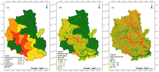
Figure 5.
(a) Spatial distribution of average annual sediment yield at subbasin scale, (b) Spatial distribution of average annual sediment yield at HRU scale, (c) Slope gradient distribution of the Takahashi catchment.
The average annual sediment yield variation between dry and wet years was significant, with 0.24 tons ha−1 yr−1 in dry years and 0.9 tons ha−1 yr−1 in wet years. In dry years, the studied catchment’s sediment yield was <1 ton ha−1 yr−1, while it increased substantially in wet years, reaching up to 3 tons ha−1 yr−1 in subbasins 6 and 19. The Takahashi tributary exhibited less variation compared to the Oda and Nariwa tributaries. The sediment yield in the Nariwa and Oda tributary subbasins increased drastically to 1.1–3 tons ha−1 yr−1 in wet years, from 0.25 and 1 ton ha−1 yr−1 in dry years. Subbasins 6 and 19 were the most critical subbasins in high precipitation as their sediment yield in wet years was nearly threefold that in the dry years (Figure S4).
3.4. Impact of Slope, Soil Type, and Land Cover on Sediment Yield Variations
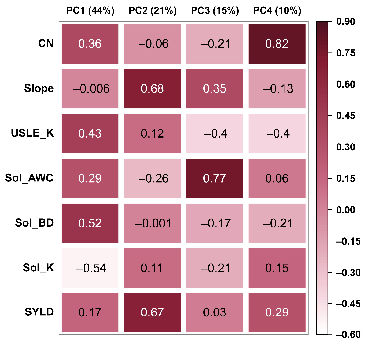
The PCA results (Figure 6) indicated that PC1 and PC2 could explain 44% and 21% of the variables. PC1 showed strong positive correlations between soil properties and CN but a weak correlation with SYLD. PC2 showed a strong positive correlation between Slope and SYLD, indicating that, as the slope increases, the sediment yield increases. PC3 explained the correlations between Sol_AWC and Slope, but this combination showed the weakest correlation with SYLD among all PCs. PC4 showed the second-strongest positive correlation between CN and SYLD after PC2. Therefore, Slope and CN influence sediment yield the most.
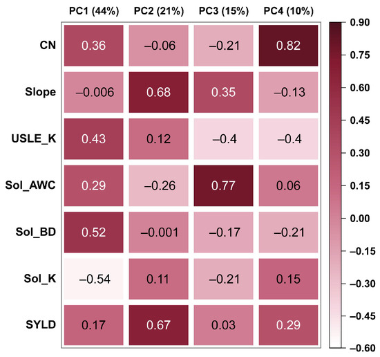
Figure 6.
Correlation coefficients of the principal components.
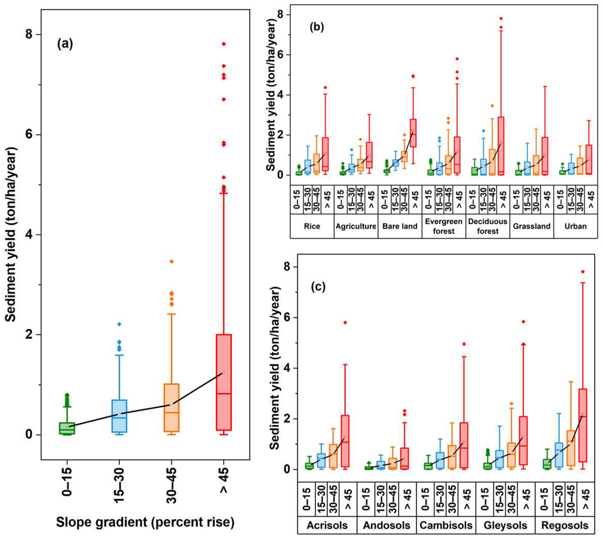
The variations in slope gradient effects on sediment yield are illustrated in Figure 7, where the average sediment yield of the slope gradients 0–15%, 15–30%, 30–45%, and >45% were 0.15, 0.42, 0.6, and 1.25 tons ha−1 yr−1, respectively (Figure 7a). Overall, sediment yields were noticeably higher in the steeper slope classes for all types of land cover (Figure 7b). Among all the types of land cover, bare land at a slope of >45% indicated the highest average sediment yield at 2.2 tons ha−1 yr−1. Rice, agricultural, and bare land had the highest sediment yield variations against the slope gradient increase. In contrast to bare and agricultural lands, urban areas showed the fewest sediment yield variations against the slope gradient, which is potentially due to infrastructure that can reduce erosion, such as stormwater management systems. Deciduous forests, evergreen forests, and grasslands had comparatively modest sediment yield. Between the major land cover types—deciduous and evergreen forests—of the studied catchment, the difference in sediment yield was significant. Evergreen forests had a higher sediment yield than deciduous forests, with an increase in slope gradient. However, deciduous forests revealed a notably large range of sediment yield as they became steeper, with the sediment yield reaching as high as 7.2 tons ha−1 yr−1.

Figure 7.
Sediment yield by slope gradient (a) without consideration of different land cover and soil types (b) for different types of land cover (c) for different soil types.
The sediment yield variations by slope gradients at different soil types are shown in Figure 7c. Acrisols, cambisols, and gleysols showed a steady increase in sediment yield with an increasing slope gradient. The sediment yield in andosols increases slowly with increasing slope gradient. Regosols showed a drastic increase in sediment yield with slope steepness, with an average sediment yield of 0.23, 0.66, 1, and 2.1 tons ha−1 yr−1 with slope 0–15%, 15–30%, 30–45%, and >45%, respectively.
4. Discussion
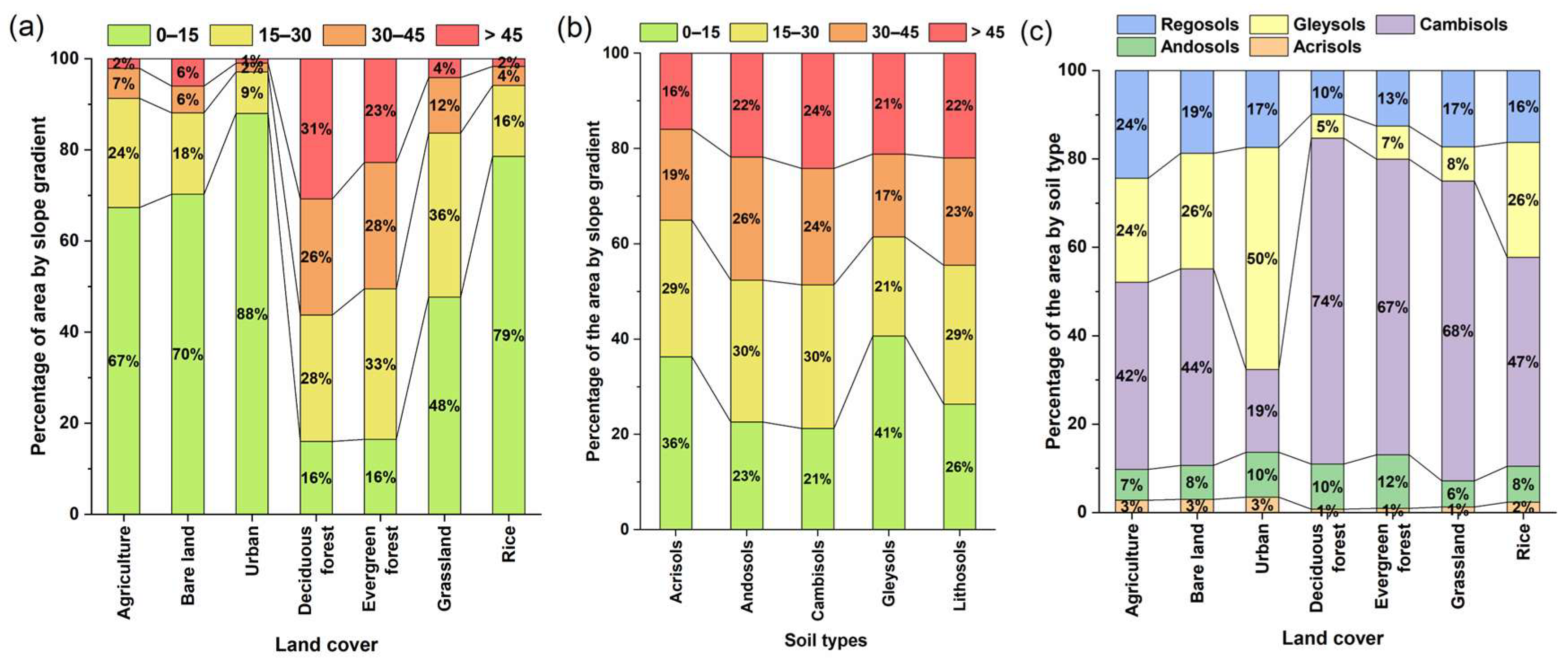
High sediment yield for the steep slopes of deciduous forests can be influenced, notwithstanding the fact that 31% of this land area type is within the slope gradient of >45%, whereas that of evergreen forests is 23% (Figure 8a). Moreover, deciduous forests showed a broad range in sediment yield with increasing slope (Figure 7b), indicating that for steeper slopes, although most of the deciduous forest has low sediment yield, extreme sediment yield occurs in some parts. Therefore, the deciduous forest steep slope gradient (>45%) in the studied catchment should be prioritized for implementing soil conservation measures. Besides the slope gradient, the high variation in sediment yield of the deciduous forest could be due to external factors arising from forest management activities. Forest management operations like fewer or no thinning operations result in higher soil loss [53]. The forest environmental conditions related to forest management (stand height, species composition and density, root density, litter, and understory vegetation) have a strong influence on sediment yield [54,55]. According to Miyata et al. [56], forest floor coverage can significantly reduce 95% of soil erosion compared to an uncovered forest. The external factors discussed in this section could not be modeled because of the unavailability of detailed data for such a large-scale catchment.
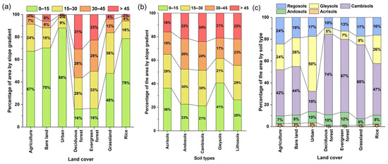
Figure 8.
(a) Land cover area percentage distribution per slope gradient (b) Soil type area percentage distribution per slope gradient (c) Soil type area percentage for each type of land cover.
Besides the slope gradient, the erosion potential of different soil types is closely related to soil properties and external conditions like climate and land use. Regosols showed the highest sediment yield with slope increase (Figure 7c), as a soil’s aggregate stability is positively correlated with its organic matter, and regosols are the soil type with the least organic matter [13,57]. Apart from their soil properties, the high sediment yield of regosols can be closely related to land cover, as regosols are primarily found in agricultural and bare lands showing higher sediment yield against the slope (Figure 8c). Meanwhile, andosols have the lowest sediment yield, although 48% of these are found within the slope gradient >30% (Figure 8b), primarily because andosols are derived from volcanic materials and have high porosity and water infiltration capacity.
The SWAT model uses meteorological data, soil type, land cover, and topography as primary input. Therefore, geological and rock types were not considered in the model. However, based on our field observation, geological influence on the hydrological system of the studied catchment can be observed (Figure 2). Therefore, the parameters influencing groundwater flow, specifically for the limestone-dominated regions, were calibrated. If information on geological and rock types can be integrated into the model simulation of a future study, it may improve the model accuracy. Furthermore, we investigated the sediment yield variations using slope gradient classes for different land cover and soil types. However, the synergistic effect of land cover and soil type on sediment variation by different slopes was not considered in the scope of this study. Moreover, extreme precipitation events, where the slope effects can become severe to trigger landslides, gullies, and streambank erosion, cannot be simulated by the standard SWAT used in this study.
5. Conclusions
The SWAT model was used to simulate the spatial distribution of high sediment yield areas and evaluate slope gradient effects for different land cover and soil types in a steep mountainous catchment. The model was calibrated and validated in daily time steps with the observed data and identified the high-sediment-yield areas. The SWAT model simulated the streamflow and sediment yield satisfactorily.
Annual precipitation variation substantially influenced annual sediment yield, especially in the western parts of the catchment. Dry years reduced the sediment yield to <1 ton ha−1 yr−1. However, it increased considerably with high precipitation, causing a threefold increase in the sediment yield in high-sediment-yield subbasins during wet years. PCA on land use, slope, and soil components showed that high sediment yield is strongly correlated with the steepness of the slope in the studied catchment. The effects of slope gradient on sediment yield are significant in areas with non-forested land cover. Meanwhile, extreme sediment yield values are found in steeply sloped areas of deciduous forests, indicating that these are priority areas for planning and developing soil conservation measures. The sediment yield variation by slope gradient results revealed that the regosol soil type exhibited the highest sediment yield with slope steepness.
This research represents a detailed analysis of sediment yield and slope gradient for different land cover and soil types in a steep mountainous catchment. Further in-depth studies considering detailed soil detachment processes and particle size distribution for different slope gradients of each land cover and soil type will potentially be useful. The findings of this study can help plan and prepare for the prevention of high sediment yields in steep catchments.
Supplementary Materials
The following supporting information can be downloaded at: https://www.mdpi.com/article/10.3390/w16101419/s1, Figure S1. land cover types of Takahashi catchment; Figure S2. Soil types in Takahashi catchment; Figure S3. Daily average precipitation across the Takahashi catchment; Figure S4. Comparison of annual sediment yield variation between (a) dry years and (b) wet years; Figure S5. Eigenvalues and explained variance by principle components; Figure S6. Correlation matrix of the identified components; Table S1: Calibrated parameters for streamflow and sediment.
Author Contributions
Conceptualization, S.-i.O.; formal analysis, Y.W.N.; funding acquisition, S.-i.O.; resources, Y.S. and M.S., supervision, S.-i.O., visualization, Y.W.N., K.W., S.-i.O., Y.S. and M.S.; writing—original draft, Y.W.N.; writing—review and editing, K.W., S.-i.O., Y.S. and M.S. All authors have read and agreed to the published version of the manuscript.
Funding
This study was supported by the Asia-Pacific Network for Global Change Research (APN) Grant No. CRRP2019-09MY-Onodera, Grant-in-Aid for Scientific Research (A) by Japan Society for the Promotion of Science (JSPS) KAKENHI Project No. 18H04151, and Japan International Cooperation Agency (JICA) Agriculture Studies Networks for Food Security (Agri-Net) program (D2102330).
Data Availability Statement
The data presented in this study are available on request from the corresponding author.
Acknowledgments
The authors thank the Takahashi River Dam Integrated Management Office for providing the daily discharge data from dams and the Okayama River Management Office for providing suspended sediment (SS) data for the Takahashi River. We would like to thank Fumio Kawahara and Sharon Bih Kimbi for their valuable suggestions and feedback during the preparation of this manuscript.
Conflicts of Interest
The authors declare no conflicts of interest.
References
- Borrelli, P.; Robinson, D.A.; Panagos, P.; Lugato, E.; Yang, J.E.; Alewell, C.; Wuepper, D.; Montanarella, L.; Ballabio, C. Land use and climate change impacts on global soil erosion by water (2015–2070). Proc. Natl. Acad. Sci. USA 2020, 117, 21994–22001. [Google Scholar] [CrossRef] [PubMed]
- Kirkby, M.J.; Morgan, R.P.C. Soil Erosion; Wiley: New York, NY, USA; Chichester, UK, 1980. [Google Scholar]
- Wuepper, D.; Borrelli, P.; Finger, R. Countries and the global rate of soil erosion. Nat. Sustain. 2019, 3, 51–55. [Google Scholar] [CrossRef]
- Barten, P.K.; Ernst, C.E. Land conservation and watershed management for source protection. J. Am. Water Works Assoc. 2004, 96, 121–135. [Google Scholar] [CrossRef]
- Marden, M. Effectiveness of reforestation in erosion mitigation and implications for future sediment yields, east coast catchments, New Zealand: A review. N. Z. Geogr. 2012, 68, 24–35. [Google Scholar] [CrossRef]
- Webb, A.A.; Dragovich, D.; Jamshidi, R. Temporary increases in suspended sediment yields following selective eucalypt forest harvesting. For. Ecol. Manag. 2012, 283, 96–105. [Google Scholar] [CrossRef]
- Sun, W.; Niu, X.; Wang, Y.; Yin, X.; Teng, H.; Gao, P.; Liu, A. Effects of forest age on soil erosion and nutrient loss in Dianchi watershed, China. Environ. Monit. Assess. 2023, 195, 340. [Google Scholar] [CrossRef] [PubMed]
- Wang, K.; Onodera, S.; Saito, M.; Shimizu, Y. Assessment of nitrogen budget in detailed spatial pattern using high precision modeling approach with constructed accurate agricultural behavior. Sci. Total Environ. 2024, 912, 169631. [Google Scholar] [CrossRef]
- Brooks, K.N.; Ffolliott, P.F.; Gregersen, H.M.; Thames, J.L. Hydrology and the Management of Watersheds; Iowa State University Press: Ames, IA, USA, 1991. [Google Scholar]
- Hancock, G.R.; Hugo, J.; Webb, A.A.; Turner, L. Sediment transport in steep forested catchments—An assessment of scale and disturbance. J. Hydrol. 2017, 547, 613–622. [Google Scholar] [CrossRef]
- Tabari, H. Climate change impact on flood and extreme precipitation increases with water availability. Sci. Rep. 2020, 10, 13768. [Google Scholar] [CrossRef]
- Zhang, X.; Yu, G.Q.; Li, Z.B.; Li, P. Experimental study on slope runoff, erosion and sediment under different vegetation types. Water Resour. 2014, 28, 2415–2433. [Google Scholar] [CrossRef]
- Defersha, M.B.; Melesse, A.M. Effect of rainfall intensity, slope and antecedent moisture content on sediment concentration and sediment enrichment ratio. Catena 2012, 90, 47–52. [Google Scholar] [CrossRef]
- Igwe, P.U.; Onuigbo, A.A.; Chinedu, O.C.; Ezeaku, I.I.; Muoneke, M.M. Soil erosion: A review of models and applications. Int. J. Adv. Eng. Res. Sci. 2017, 4, 138–150. [Google Scholar] [CrossRef]
- Pijl, A.; Reuter, L.E.H.; Quarella, E.; Vogel, T.A.; Tarolli, P. GIS-based soil erosion modeling under various steep-slope vineyard practices. Catena 2020, 193, 104604. [Google Scholar] [CrossRef]
- Ketema, A.; Dwarakish, G.S. Water erosion assessment methods: A review. ISH J. Hydraul. Eng. 2021, 27, 434–441. [Google Scholar] [CrossRef]
- Pandey, A.; Himanshu, S.K.; Mishra, S.K.; Singh, V.P. Physically based soil erosion and sediment yield models revisited. Catena 2016, 147, 595–620. [Google Scholar] [CrossRef]
- Schmidt, E.; Chinowsky, P.; Robinson, S.; Strzepek, K. Determinants and impact of sustainable land management (SLM) investments: A systems evaluation in the Blue Nile Basin, Ethiopia. Agric. Econ. 2017, 48, 613–627. [Google Scholar] [CrossRef]
- Aloui, S.; Mazzoni, A.; Elomri, A.; Aouissi, J.; Boufekane, A.; Zghibi, A. A review of Soil and Water Assessment Tool (SWAT) studies of Mediterranean catchments: Applications, feasibility, and future directions. J. Environ. Manag. 2023, 326, 116799. [Google Scholar] [CrossRef] [PubMed]
- Musyoka, F.K.; Strauss, P.; Zhao, G.; Strohmeier, S.; Mutua, B.M.; Klik, A. Evaluating the impacts of sustainable land management practices on water quality in an agricultural catchment in Lower Austria using SWAT. Environ. Monit. Assess. 2023, 195, 512. [Google Scholar] [CrossRef] [PubMed]
- Wang, K.; Onodera, S.; Saito, M. Evaluation of nitrogen loading in the last 80 years in an urbanized Asian coastal catchment through the reconstruction of severe contamination period. Environ. Res. Lett. 2022, 17, 014010. [Google Scholar] [CrossRef]
- Meaurio, M.; Zabaleta, A.; Srinivasan, R.; Sauvage, S.; Sánchez-Pérez, J.M.; Lechuga-Crespo, J.L.; Antiguedad, I. Long-term and event-scale sub-daily streamflow and sediment simulation in a small forested catchment. Hydrol. Sci. J. 2021, 66, 862–873. [Google Scholar] [CrossRef]
- Marin, M.; Clinciu, I.; Tudose, N.C.; Ungurean, C.; Adorjani, A.; Mihalache, A.L.; Davidescu, A.A.; Davidescu, Ș.O.; Dinca, L.; Cacovean, H. Assessing the vulnerability of water resources in the context of climate changes in a small forested watershed using SWAT: A review. Environ. Res. 2020, 184, 109330. [Google Scholar] [CrossRef] [PubMed]
- Jimeno-Sáez, P.; Martínez-España, R.; Casalí, J.; Pérez-Sánchez, J.; Senent-Aparicio, J. A comparison of performance of SWAT and machine learning models for predicting sediment load in a forested Basin, Northern Spain. Catena 2022, 212, 105953. [Google Scholar] [CrossRef]
- Abbaspour, K.C.; Rouholahnejad, E.; Vaghefi, S.; Srinivasan, R.; Yang, H.; Kløve, B. A continental-scale hydrology and water quality model for Europe: Calibration and uncertainty of a high-resolution large-scale SWAT model. J. Hydrol. 2015, 524, 733–752. [Google Scholar] [CrossRef]
- Wang, K.; Onodera, S.; Saito, M.; Ishida, T. Assessment of long-term phosphorus budget changes influenced by anthropogenic factors in a coastal catchment of Osaka Bay. Sci. Total Environ. 2022, 843, 156833. [Google Scholar] [CrossRef] [PubMed]
- Serrao, E.A.O.; Silva, M.T.; Ferreira, T.R.; Ataide, L.C.P.; Santos, C.A.; Lima, A.M.M.; Silva, V.P.R.; Sousa, F.A.S.; Gomes, D.J.C. Impacts of land use and land cover changes on hydrological processes and sediment yield determined using the SWAT model. Int. J. Sediment Res. 2022, 37, 54–69. [Google Scholar] [CrossRef]
- Wang, W.; Xie, Y.; Bi, M.; Wang, X.; Lu, Y.; Fan, Z. Effects of best management practices on nitrogen load reduction in tea fields with different slope gradients using the SWAT model. Appl. Geogr. 2018, 90, 200–213. [Google Scholar] [CrossRef]
- Tan, M.L.; Gassman, P.W.; Srinivasan, R.; Arnold, J.G.; Yang, X. A review of SWAT studies in Southeast Asia: Applications, challenges and future directions. Water 2019, 11, 914. [Google Scholar] [CrossRef]
- Yoshida, K. Estimation of inundation area and depth distribution for the Takahashi River and Hijikawa River flooding associated with the heavy rain event of July 2018. Int. J. Remote Sens. 2018, 38, 422–425. (In Japanese) [Google Scholar]
- Amano, T.; Asai, K.; Shirozu, H.; Takabu, A.; Yamamoto, T. Influence of sediment discharge and driftwoods on Noro-gawa dam and river flooding during heavy rain in July 2018. J. Jpn. Soc. Civ. 2021, 9, 175–183. [Google Scholar] [CrossRef]
- Nihei, Y.; Shinohara, A.; Ohta, K.; Maeno, S.; Akoh, R.; Akamatsu, Y.; Komuro, T.; Kataoka, T.; Onomura, S.; Kaneko, R. Flooding along oda river due to the western Japan heavy rain in 2018. J. Disaster Res. 2019, 14, 874–885. [Google Scholar] [CrossRef]
- Shakti, P.C.; Kamimera, H.; Misumi, R. Inundation Analysis of the Oda River Basin in Japan during the Flood Event of 6-7 July 2018 Utilizing Local and Global Hydrographic Data. Water 2020, 12, 1005. [Google Scholar] [CrossRef]
- Nishimura, S.; Takeshita, Y.; Nishiyama, S.; Suzuki, S.; Shibata, T.; Shuku, T.; Komatsu, M.; Kim, B. Disaster report of 2018 July heavy rain for geo-structures and slopes in Okayama. Soils Found. 2020, 60, 300–314. [Google Scholar] [CrossRef]
- Nohara, D.; Takemon, Y.; Sumi, T. Real-time flood management and preparedness: Lessons from floods across the Western Japan in 2018. In Advances in Hydroinformatics; Springer: Berlin/Heidelberg, Germany, 2020; pp. 287–304. [Google Scholar] [CrossRef]
- Shakti, P.C.; Kamimera, H. Flooding in Oda river basin during torrential rainfall event in July 2018. Eng. J. 2019, 23, 477–485. [Google Scholar] [CrossRef]
- Wang, K.; Onodera, S.; Saito, M.; Shimizu, Y.; Iwata, T. Effects of forest growth in different vegetation communities on forest catchment water balance. Sci. Total Environ. 2022, 809, 151159. [Google Scholar] [CrossRef] [PubMed]
- Arnold, J.G.; Kiniry, J.R.; Srinivasan, R.; Williams, J.R.; Haney, E.B.; Neitsch, S.L. Soil and Water Assessment Tool Input/Output Documentation 2012; Texas Water Resources Institute Technical Report No. 439; Texas A&M University System: College Station, TX, USA, 2012. [Google Scholar]
- Neitsch, S.L.; Arnold, J.G.; Kiniry, J.R.; Williams, J.R.; King, K.W. Soil and Water Assessment Tool, Theoretical Documentation, Version 2000; TexasWater Resources Institute, Texas A&M University: College Station, TX, USA, 2002. [Google Scholar]
- Arnold, J.G.; Moriasi, D.N.; Gassman, P.W.; Abbaspour, K.C.; White, M.J.; Srinivasan, R.; Santhi, C.; Harmel, R.D.; van Griensven, A.; van Liew, M.W.; et al. SWAT: Model use, calibration, and validation. Trans. ASABE 2012, 55, 1491–1508. [Google Scholar] [CrossRef]
- Wang, K.; Onodera, S.; Saito, M.; Okuda, N.; Okubo, T. Estimation of phosphorus transport influenced by climate change in a rice paddy catchment using SWAT. Int. J. Environ. Res. 2021, 15, 759–772. [Google Scholar] [CrossRef]
- Leta, O.T.; van Griensven, A.; Bauwens, W. Effect of single and multisite calibration techniques on the parameter estimation, performance, and output of a SWAT model of a spatially heterogeneous catchment. J. Hydrol. Eng. 2017, 22, 05016036. [Google Scholar] [CrossRef]
- de Bressiani, D.A.; Gassman, P.W.; Fernandes, J.G.; Garbossa, L.H.P.; Srinivasan, R.; Bonumá, N.B.; Mendiondo, E.M. A review of soil and water assessment tool (SWAT) applications in Brazil: Challenges and prospects. Int. J. Agric. Bio. Eng. 2015, 8, 9–35. [Google Scholar] [CrossRef]
- Tuppad, P.; Douglas-Mankin, K.R.; Lee, T.; Srinivasan, R.; Arnold, J.G.; Srinivasan, R.; Member, A. Soil and Water Assessment Tool (SWAT) hydrologic/water quality model: Extended capability and wider adoption. Trans. ASABE 2011, 54, 1677–1684. [Google Scholar] [CrossRef]
- Gassman, P.W.; Sadeghi, A.M.; Srinivasan, R. Applications of the SWAT model special section: Overview and insights. J. Environ. Qual. 2014, 43, 1–8. [Google Scholar] [CrossRef]
- Gassman, P.W.; Reyes, M.R.; Green, C.H.; Arnold, J.G. The soil and water assessment tool: Historical development, applications, and future research directions. Trans. ASABE 2007, 50, 1211–1250. [Google Scholar] [CrossRef]
- Verma, S.K.; Prasad, A.D.; Verma, M.K. An assessment of ongoing developments in water resources management incorporating SWAT Model: Overview and perspectives. Nat. Environ. Pollut. Technol. 2022, 21, 1963–1970. [Google Scholar] [CrossRef]
- Tan, M.L.; Gassman, P.W.; Yang, X.; Haywood, J. A review of SWAT applications, performance and future needs for simulation of hydro-climatic extremes. Adv. Water Resour. 2020, 143, 103662. [Google Scholar] [CrossRef]
- Moriasi, D.N.; Gitau, M.W.; Pai, N.; Daggupati, P. Hydrologic and water quality models: Performance measures and evaluation criteria. Trans. ASABE 2015, 58, 1763–1785. [Google Scholar] [CrossRef]
- Ashine, E.T.; Tadesse Bedane, M. Most Sensitive Parameters of Soil and Water Assessment Tool (SWAT) Hydrological Model: A Review. AOMB 2022, 3, 000558. [Google Scholar] [CrossRef]
- Wang, Y.; Shao, J.; Su, C.; Cui, Y.; Zhang, Q. The application of improved SWAT model to hydrological cycle study in karst area of south China. Sustainability 2019, 11, 5024. [Google Scholar] [CrossRef]
- Wang, K.; Onodera, S.; Saito, M.; Shimizu, Y. Long-term variations in water balance by increase in percent imperviousness of urban regions. J. Hydrol. 2021, 602, 126767. [Google Scholar] [CrossRef]
- Razafindrabe, B.H.N.; He, B.; Inoue, S.; Ezaki, T.; Shaw, R. The role of forest stand density in controlling soil erosion: Implications to sediment-related disasters in Japan. Environ. Monit. Assess. 2010, 160, 337–354. [Google Scholar] [CrossRef]
- Shinohara, Y.; Misumi, Y.; Kubota, T.; Nanko, K. Characteristics of soil erosion in a moso-bamboo forest of western Japan: Comparison with a broadleaved forest and a coniferous forest. Catena 2019, 172, 451–460. [Google Scholar] [CrossRef]
- Wen, Z.; Zheng, H.; Zhao, H.; Liu, L.; Ouyang, Z. Species compositional, structural and functional diversity exerts different effects on soil erosion caused by increased rainfall intensity in Chinese tropical forests. Plant Soil 2021, 465, 97–108. [Google Scholar] [CrossRef]
- Miyata, S.; Kosugi, K.; Gomi, T.; Mizuyama, T. Effects of forest floor coverage on overland flow and soil erosion on hillslopes in Japanese cypress plantation forests. Water. Resour. Res. 2009, 45, W06402. [Google Scholar] [CrossRef]
- Parwada, C.; Van Tol, J. Soil properties influencing erodibility of soils in the Ntabelanga area, Eastern Cape Province, South Africa. Acta Agric. Scand. B Soil Plant Sci. 2017, 67, 67–76. [Google Scholar] [CrossRef]
Disclaimer/Publisher’s Note: The statements, opinions and data contained in all publications are solely those of the individual author(s) and contributor(s) and not of MDPI and/or the editor(s). MDPI and/or the editor(s) disclaim responsibility for any injury to people or property resulting from any ideas, methods, instructions or products referred to in the content. |
© 2024 by the authors. Licensee MDPI, Basel, Switzerland. This article is an open access article distributed under the terms and conditions of the Creative Commons Attribution (CC BY) license (https://creativecommons.org/licenses/by/4.0/).

