Article

An Efficient Water Quality Prediction and Assessment Method Based on the Improved Deep Belief Network—Long Short-Term Memory Model

1
School of Computing and Artificial Intelligence, Beijing Technology and Business University, No. 11/33 FuCheng Road, HaiDian District, Beijing 100048, China
2
Beijing Laboratory for Intelligent Environmental Protection, Beijing 100048, China
3
School of Automation, Beijing Institute of Technology, Beijing 100081, China
*
Author to whom correspondence should be addressed.
Water 2024, 16(10), 1362; https://doi.org/10.3390/w16101362
Submission received: 1 April 2024 / Revised: 8 May 2024 / Accepted: 9 May 2024 / Published: 11 May 2024

Abstract

:
The accuracy of water quality prediction and assessment has always been the focus of environmental departments. However, due to the high complexity of water systems, existing methods struggle to capture the future internal dynamic changes in water quality based on current data. In view of this, this paper proposes a data-driven approach to combine an improved deep belief network (DBN) and long short-term memory (LSTM) network model for water quality prediction and assessment, avoiding the complexity of constructing a model of the internal mechanism of water quality. Firstly, using Gaussian Restricted Boltzmann Machines (GRBMs) to construct a DBN, the model has a better ability to extract continuous data features compared to classical DBN. Secondly, the extracted time-series data features are input into the LSTM network to improve predicting accuracy. Finally, due to prediction errors, noise that randomly follows the Gaussian distribution is added to the assessment results based on the predicted values, and the probability of being at the current water quality level in the future is calculated through multiple evolutionary computations to complete the water quality assessment. Numerical experiments have shown that our proposed algorithm has a greater accuracy compared to classical algorithms in challenging scenarios.

1. Introduction

The recent development of society and the economy has brought an improvement in the quality of life, a constantly increasing degree of industrialization, and the pursuit of various benefits while ignoring the natural ecological environment, species diversity, and other ecological issues, which has led to the problems of ecological imbalance, high water pollution, water resource shortage, species reduction, and other adverse consequences. At present, multiple regions of the world are in a state of water shortage. For example, the per capita water consumption in China is only 2300 cubic meters, less than a quarter of the global average level [1,2,3]. Water pollution will further exacerbate the shortage of water sources. Simultaneously, drinking contaminated water can endanger human lives, and it is estimated that about 190 million people fall ill every year as a result, and nearly 6 million of them die from some kind of disease. In addition, the phenomenon of water blooming could eventually cause the disappearance of many animal and plant species in the water ecosystem and destroy the ecological balance [4]. Evidently, the loss of personal safety caused by water pollution is immeasurable. Therefore, the analysis of the factors causing water pollution and the prediction of the trend of water quality change will provide an effective basis for the prevention and control of water pollution, which will be of great significance for the protection of species diversity and human life activities. Water quality prediction represents the prediction of the evolution of elements that affect water quality over a certain period in the future using water quality models and data obtained using water quality measurements. At present, the existing water quality prediction methods can mainly be divided into two categories: water quality prediction methods based on mechanism models and water quality prediction methods based on data-driven models [5,6].
(1)
Water quality prediction methods based on mechanism models
The water quality prediction methods based on mechanistic models mainly determine water quality using a mathematical model of the assessment of various elements in the water. The advantage of these methods is that their parameters are easy to tune and express, and they have a very clear physical meaning; also, the prediction model is robust and adaptable. Commonly used mechanism models generally include the MIKE model, CE-QUAL-W2 model, EFDC model, and WASP model [7,8,9,10]. However, due to the complex internal mechanism of some water bodies, it is difficult and time-consuming to directly describe the evolution process of water quality with mathematical expressions. Besides that, it is difficult to determine the value of some structural variables directly, which limits the practical application of these methods. Namely, if the parameters of the mathematical model are not well tuned or there are large errors, the accuracy of the model will be seriously affected.
(2)
Water quality prediction methods based on data-driven models
Data-driven models are constructed using a large amount of data for model development and training. The main advantage of methods based on data-driven models is that they can accurately predict the “black box” events and are suitable for systems whose internal mechanisms are too complex to be described using mathematical expressions. Data-driven models have been widely used in many fields since they can learn data relationships using various types of neural network models [11]. In [12], the long short-term memory (LSTM) neural network model was used for time-series prediction, accurately revealing the future development trend of water quality and indicating the application potential of the LSTM model in drinking-water quality prediction. In [13], a data-driven method for water quality prediction and real-time warning was developed by combining an improved genetic algorithm (IGA) and a backpropagation neural network (BPNN) model. In [14], a task-oriented adaptive radial basis function (ATO-RBF) network was proposed to design the prediction model, which can obtain the effluent biochemical oxygen demand (BOD) and effluent total nitrogen (TN) accurately and timely. The above studies can quickly and accurately establish water quality prediction models by mining potential connections between data without any prior knowledge. In all, data-driven water quality models have been widely used and are not influenced by geographical and environmental factors of water bodies but require extensive and high-quality actual water quality measurement data to train the models. If the quality of the obtained data is low, the accuracy of the model will be seriously affected.
Water quality assessment refers to the selection of the corresponding water quality parameters, water quality content standards, and other related parameters according to the required evaluation objectives in the field of water quality. Currently, the existing water quality assessment methods can be roughly divided into three main categories. The first category evaluates water quality by measuring biochemical elements in the water [15]. In this category, model evaluation processes are performed by analyzing the ecological conditions of water quality and the relationships between pollutants and organisms in the water. The second category is based on the nutritional status index, which is used to evaluate the water quality indicators, and commonly used indicators include the trophic status index (TSI), trophic level index (TLI), and water quality index (WQI). In [16,17,18,19,20,21], the WQI was used to evaluate water quality. The WQI was defined by the National Foundation of Health (NSF). The initial WQI values range from 0 to 100 and are calculated based on nine variables: dissolved oxygen (DO), BOD, nitrate, phosphate, fecal coliform, pH value, temperature, turbidity, and total solids. In [16], an extensive review of water quality index models is provided, covering a variety of models and their use in surface water quality assessment. In [17], the use of the WQI method to assess the overall quality of the water, using various parameters to assess Poyang Lake, helps to understand the current state of Poyang Lake’s water quality and can provide insights on potential environmental impacts and human health issues. In [18], the water quality of lakes is assessed using the WQI method, and the multivariate analysis technique is used to gain an in-depth understanding of the water quality status and the possible influencing factors. In [19], this paper proposes a dynamic water quality index model based on a functional data analysis to better understand water quality change and its influencing factors. In [20], this paper aims to investigate the overall water quality of Skardu spring water using the WQI method. In [21], the study used a composite WQI and a self-organizing map (SOM) to assess water quality in river catchments. In general, the WQI combines several water quality parameters to provide an assessment of the overall picture of water quality. However, the weight setting and parameter selection may be affected by subjective factors, resulting in the deviation of results. Another important index method for assessing water quality is TSI. In [22,23,24], the authors adopted the TSI based on transparency and combined it with the content of total phosphorus (TP) and chlorophyll (Chl-a) to calculate and classify the lake water quality into four basic types: lean nutrient type, medium nutrient type, eutrophic type, and excessive eutrophic type. In the future, an improved TSI index could be defined to evaluate the nutritional status of water quality more accurately. To sum up, TSI addresses specific problems: it is used to assess the degree of eutrophication of water bodies and provides specific indicators for water ecosystems. In contrast to WQI, TSI focuses on eutrophication and cannot provide a comprehensive assessment of overall water quality. The third category uses neural networks to process data, learn informative features, construct non-linear relationships between various pieces of information, and evaluate water quality. Based on the Monte Carlo method, a two-dimensional hydrodynamic uncertainty eutrophication model was constructed [25] to reproduce the observed water temperature, nutrients, and algae conditions accurately. This method has shown a reasonable numerical representation ability of the actual hydrodynamic and eutrophication dynamics of a lake. It should be noted that the internal mechanism of water quality is relatively complex, so the criteria used in evaluation methods can vary. Namely, each of the evaluation methods has its own advantages, and an appropriate method should be determined in a comprehensive way by jointly considering the climatic environment, geographical location, biological status, and human factors.
Most of the existing water quality modeling or time-series predicting methods are based on the mechanism or the LSTM model [7,8,9,10,26]. This paper not only avoids the complexity of constructing a mechanistic model but also extracts data features to reduce the dependence on data quality, which proposes an improved deep belief network (DBN) and LSTM fusion method to construct a water quality prediction model based on a data-driven approach, and constructs a DBN with Gaussian Restricted Boltzmann Machines (GRBMs) stacking to improve the algorithm, noted as GDBN, which solves the problem of data loss in the feature extraction of the classical DBN neuron binary problem. Firstly, the DBN is constructed using GRBMs to extract data features; secondly, the extracted time-series data features are input into the LSTM network, and the prediction accuracy is improved using the ability of LSTM to store time-series information; finally, due to the prediction error, assessment results based on the predicted values are added to the random noise obeying Gaussian distribution, and the probability of being at the current water quality level in the future is calculated through multiple evolutionary calculations to achieve water quality health assessment and risk management. Numerical experimental results show that the algorithm proposed in this paper has good accuracy in challenging scenarios.
The rest of this paper is organized as follows. In Section 2, the basic principles of the LSTM and DBN networks used to design the proposed improved DBN-LSTM prediction model are introduced. In Section 3, the GDBN-based modeling approach is proposed, and the prediction method based on the GDBN-LSTM model is described in detail. Two experiments are shown in Section 4 and the main conclusions are presented in Section 5.

2. LSTM and DBN Networks

2.1. LSTM Network

LSTM is a temporal recurrent neural network, a variant recurrent neural network (RNN) designed to solve the problem of RNNs being unable to handle long-term memory. The LSTM is suitable for handling and predicting time-based problems. The main advantage of LSTM is that it can ensure long-term memory so that the problems of gradient disappearance and explosion in classical RNNs can be solved [26]. The structure of LSTM is shown in Figure 1.
In Figure 1, x t denotes the network input of the current moment, h t 1 , is the external state of the memory unit at the previous moment, and c t is the internal state of the memory unit at the previous moment. The LSTM adds a new memory unit to store long-term memory, but this increases the complexity of the LSTM structure [27]. The LSTM has three gate units, namely the forget gate, input gate, and output gate, which are, respectively, defined as follows:
(1)
Forget gate: In this gate, it is decided with a certain probability whether to forget the previous layer of the hidden neuron cell state or not, and the corresponding mathematical expression is given by
f ( t ) = σ ( w f h t 1 + U f x t + b f )
(2)
Input gate: This gate handles the input for the current sequence position, and it is defined as follows:
i ( t ) = σ ( w i h t 1 + U i x t + b i )
(3)
Output gate: The output at moment t 1 depends on the implicit state h t 1 and the current input x t , which can be expressed as follows:
O ( t ) = σ ( w 0 h t 1 + U 0 x t + b 0 )
The candidate state can be calculated by
C ( t ) = tanh ( w c h t 1 + U c x t + b c )
The updated cell state is calculated by
C ( t ) = C ( t 1 ) f ( t ) + i ( t ) C ( t )
The current external state is given by
h ( t ) = O ( t ) tanh ( C ( t ) )

2.2. DBN Network

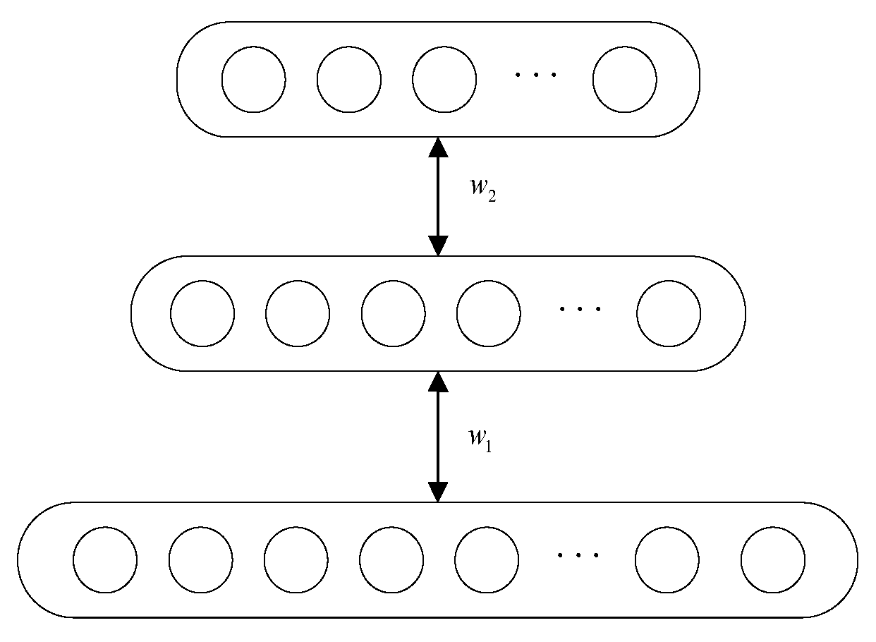
A deep confidence network represents a deep probabilistic digraph model whose structure is composed of multiple layers composed of a different number of neurons. There is no connection between the nodes in the same layer, and they are independent of each other. The neurons of two adjacent layers are fully connected; the lowest layer of this neural network is a visible layer, which is used to input data features, and the other layers denote hidden layers. The connection between the layers is from top to bottom [28]; a simplified structure of a deep confidence network is shown in Figure 2.
For a DBN with m layers, the bottom layer is considered the visible layer and is used to input sample features. The connection of the top two layers of neurons is bidirectional and can be regarded as two layers in the RBM structure, which are used to generate the probability of the previous layer of neurons. In addition to the interconnection of neurons at the top two layers of the DBN structure, the probability of variables at each layer being opened depends on variables at the upper layer. Each layer of the deep confidence network can be regarded as a sigmoid confidence block. During sample generation, a restricted Boltzmann machine on the top layer is run first several times during the Gibbs sampling until the heat is balanced [29]. The expression of the energy function to reach thermal equilibrium is as follows:
E ( v , h ) = a T v b T v v T w h
where v is visible units, h is hidden units, w is the weight between v and h , and a and b are the bias of the visible units and hidden units, respectively.
When equilibrium is reached, the probability value of the next hidden layer is generated, and the conditional distribution sampling of variables in each layer is performed successively. The formula for the joint probability distribution of the visible and hidden layers is as follows:
p ( v , h ) = e E ( v , h ) v h e E ( v , h )
When the value of the upper-layer neuron is given, the value of the lower-layer neuron is conditionally independent of it, so it can be independently sampled. The sampling process is as follows.
The probability of hidden-layer neurons being activated is calculated by
p ( h j | v ) = σ ( b j + j w i j v i )
The probability that the visible-layer neuron is activated via the hidden-layer neuron is given by
p ( v i | h ) = σ ( a i + j w i j h j )
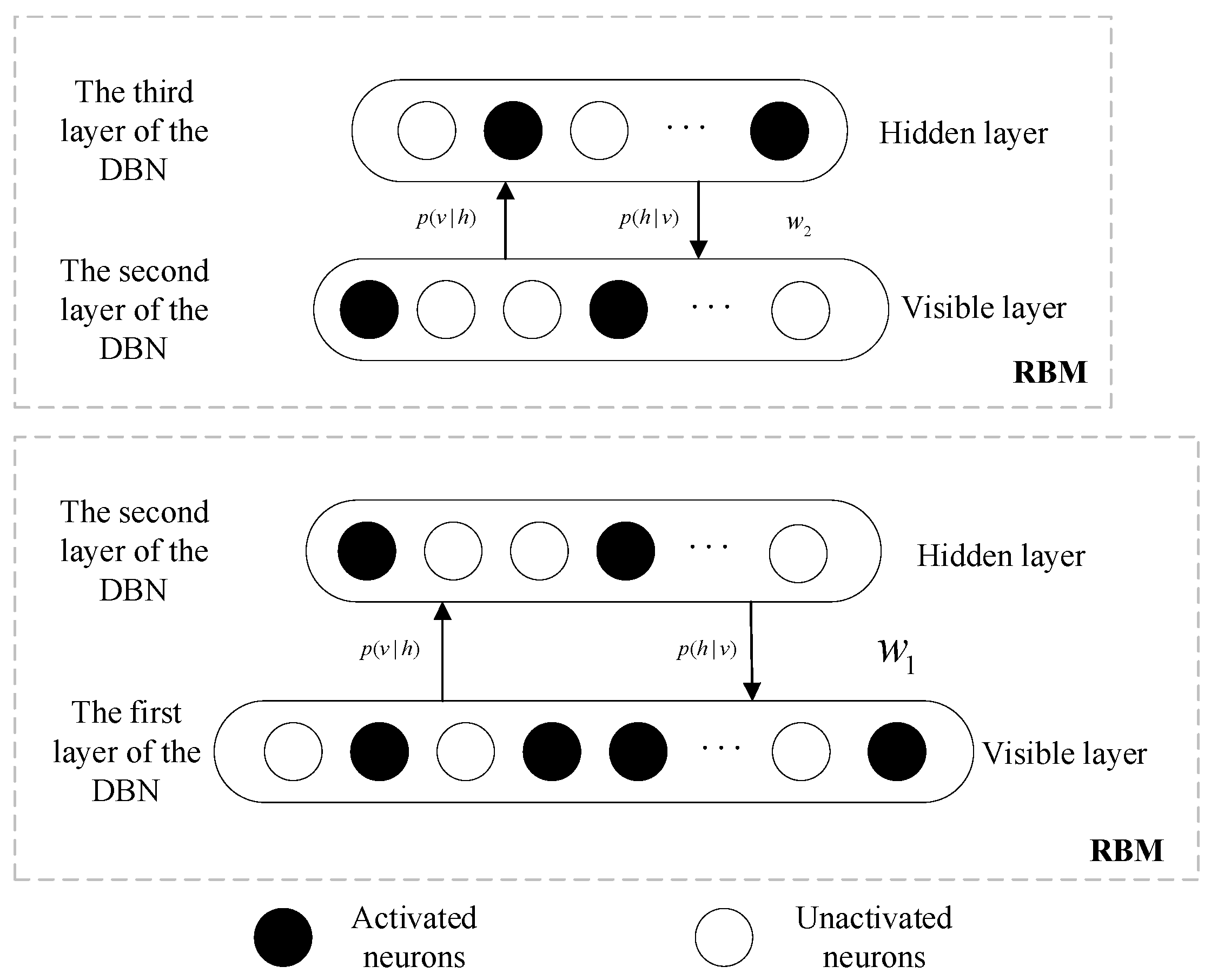
where σ is the sigmoid activation function, but other logistic functions could also be used as an activation function. The same-layer neurons are independent of each other, so the probability density also has the characteristic of independence. The training process is shown in Figure 3.
DBN layer-by-layer pre-training method: First, define the training set, learning rate, network layer number, weights, and biases; the weights and biases are initialized, where the bias initialization is set to zero and the weights are initialized to generate random numbers that conform to a normal distribution with a zero mean and a variance of 0.1. Next, sample the hidden variables from the training set, calculate the probability and value of the hidden variables at the next layer based on the hidden variables at the current layer, and repeat this process until the last layer is reached. After that, the implicit variable of the penultimate layer is taken as a training sample, and the last layer is trained with a restricted Boltzmann machine to obtain the training weight and bias values [30].
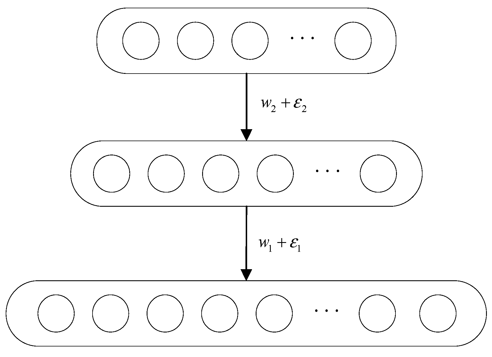
To make the model converge to a local optimum faster, the DBN performs the fine adjustment of weights, and the connection weight between every two layers can be expressed as a combination of the downward generation matrix and the upward cognitive matrix. The fine-tuning process is presented in Figure 4. The main goal is to calculate the probability of the upper layer of the upward cognitive weight matrix for sampling and modify the generated weight matrix to make its probability reach the maximum. When the RBM of the top layer reaches the thermal equilibrium, by generating the weight matrix and calculating the cognitive weight matrix in turn, the upward conditional probability is maximized [31].

3. Proposed GDBN-LSTM Model

3.1. GDBN Model

When ordinary DBN trains RBM layer by layer, the hidden-layer RBM is binary, which can extract data features but is prone to information loss. So, the DBN with Gaussian RBM is proposed to train the network, noted as GDBN. First, the DBN with Gaussian RBM stacking is more suitable for continuous variables because GRBM is a restricted Boltzmann machine that can be used to process real-valued features. In practical applications, much of the data is of a continuous type, such as pixel values in images and sample values in audio. Therefore, using a GRBM instead of the traditional binary RBM can better handle these continuous variables. The second is a more accurate feature representation: because a GRBM can better model real distributions, the implicit feature representations it generates are typically more accurate than a binary RBM. This can help improve performance, for example, in tasks such as classification, clustering, or data dimensionality reduction; it can also effectively suppress overfitting. Compared with the traditional binary RBM, the probability density function of a GRBM has more degrees of freedom and can better represent the complex structure of the data. This can make the model more flexible and help suppress the overfitting phenomenon.
The expression of the energy function of a GRBM is as follows:
E ( v , h ) = i = 1 n v ( v i a i ) 2 2 σ i 2 j = 1 n h ( h j b j ) 2 2 σ j 2 i = 1 n v j = 1 n h ( v i a i ) ( h j b j ) σ i σ j w i j
where v is the visible-layer neuron state vector; h is the hidden-layer neuron state vector; a i and b j are the bias parameters of the i and j neurons in v and h , respectively; n v and n h are the number of neurons in the visible and hidden layers, respectively; σ i 2 and σ j 2 are the noise variances of the i and j neurons in the visible and hidden layers, respectively; and w i j is the weight of the neuron connecting the i visible layer and the j hidden layer.
The improvement process of DBN is to choose the positive-etheric distribution function at the time of sampling, which is calculated as follows:
p ( x i = x | x / i ) = 1 2 π σ 2 exp ( ( x μ ) 2 σ 2 )
where μ is the parameter learned from the GRBM network, which can be calculated from the current state x i and σ  is 1.
The conditional probability formula for the explicit layer to the hidden layer in GRBM is as follows:
p ( v i | h ) = N ( a i + j w i j h j , 1 )
The conditional probability formula of the hidden layer to the explicit layer in GRBM is as follows:
p ( h j | v ) = N ( b j + i w j i v i , 1 )

3.2. GDBN-LSTM Design

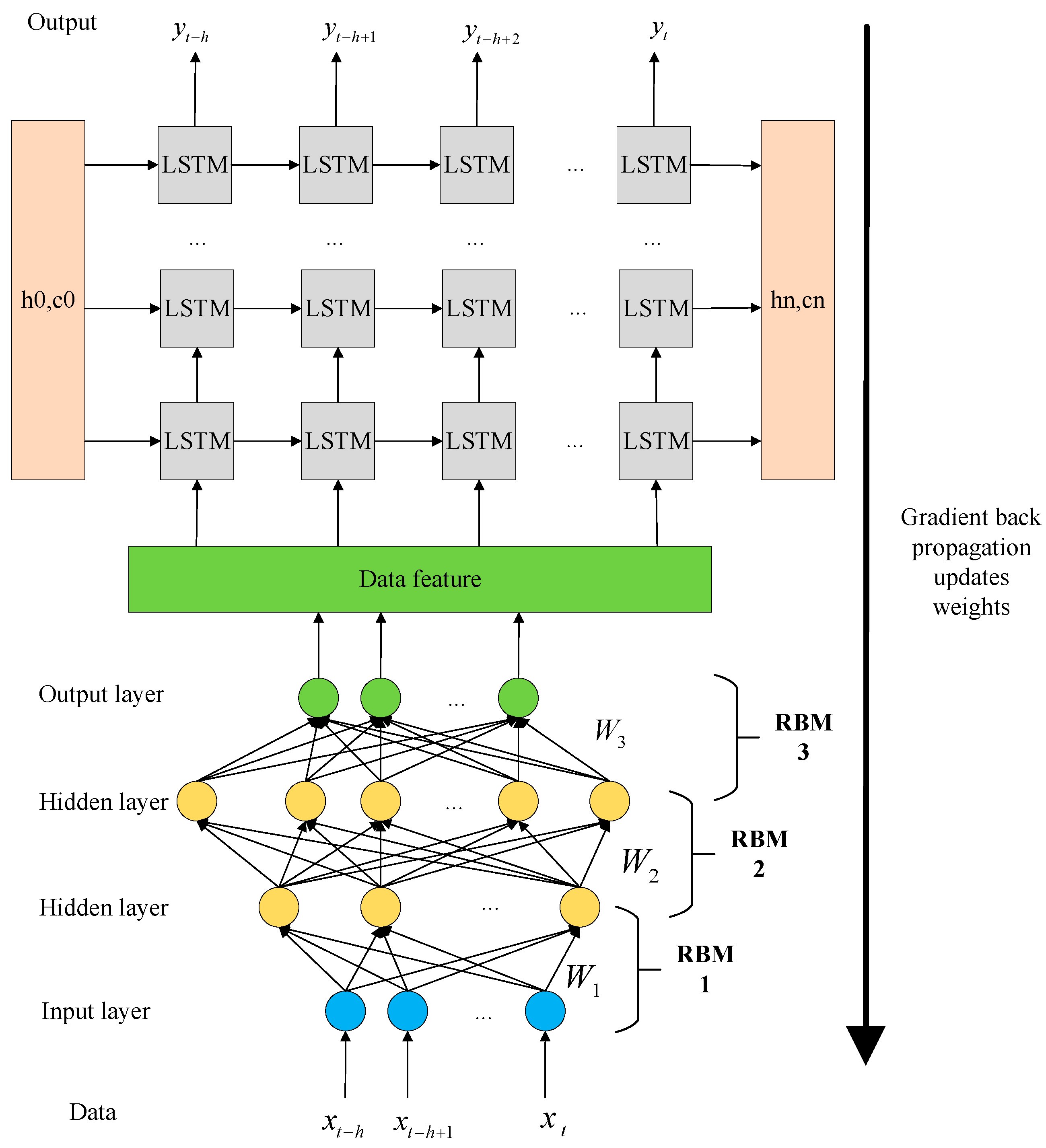
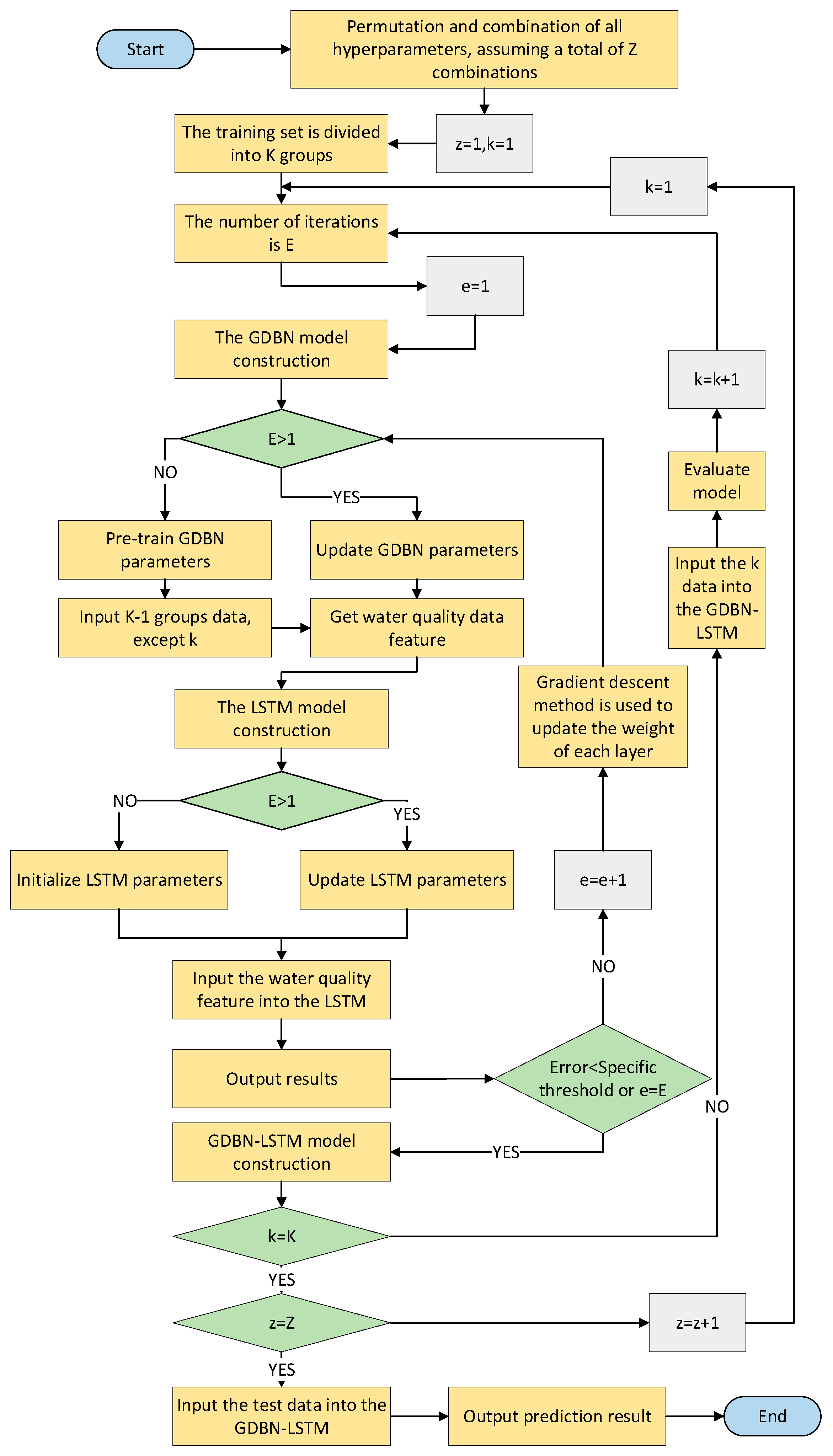
The proposed prediction model uses the GDBN model to mine the essential characteristics of water quality time-series data and inputs them into the LSTM network for prediction. First, the DBN model is used for pre-training, and the contrastive divergence (CD) algorithm was used to train RBM in a layer-by-layer manner using Gibbs sampling to obtain the weights between layers and extract the basic information reflecting the change in water quality characteristics. After that, the features are input into the LSTM to predict the next time sequence according to the hidden units and memory units in the neural network. The network model is shown in Figure 5.
The specific steps are as follows:
Step 1: Methods for determining hyperparameters: The values of different hyperparameters are selected, and the mesh search method and K-fold cross-validation are used to determine the most hyperparameter combinations.
Step 2: GDBN model construction: The weights and thresholds of the GDBN layer are initialized and the data are pre-trained using the CD algorithm with one-step Gibbs sampling.
Step 3: LSTM model construction: The input layer of the LSTM is used to receive the characteristics of the pre-trained GDBN model’s output. The last LSTM layer is a full connection layer, and it outputs the final desired dimension.
Step 4: GDBN-LSTM model construction: Because the GDBN model adopts a greedy algorithm, the weight of each layer converges to a local optimum rather than to the global optimal value, so the backpropagation algorithm is adopted to calculate the gradient layer by layer for the overall fine-tuning of the model and parameter update; this process represents supervised learning.
Here are the specific steps for the training process:
Step 4.1: Initialization parameters: Using the pre-training method of GDBN, the weight matrix and bias vector are trained and used to initialize the hidden layer separation unit of the LSTM.
Step 4.2: Forward propagation: The input sequence X is forward propagated to the LSTM layer, to obtain the corresponding output feature vector with the recurrent neuron hidden state; the feature representation vector extracted using the DBN model is obtained.
Step 4.3: Present the fused features: For example, splice the hidden state of the LSTM layer with the DBN-extracted feature vector into a brand-new tensor and go to the next step.
Step 4.4: Fine-tune the model parameters: Take the paper’s own parameters that need to be optimized, define the loss function with the desired values, and update the paranoia terms and weight matrix using standard backpropagation techniques.
Step 4.5: Calculate the error and update: The gradient of the selected loss function is calculated and then all adjustable parameters are updated iteratively inside the network using a learning algorithm.
The flowchart of the proposed algorithm is shown in Figure 6.

3.3. Water Quality Assessment Method

3.3.1. Single-Factor Index Evaluation Method

Due to the condition of water quality collection equipment and the problem of a variable water quality environment, it is challenging to achieve accurate and comprehensive water quality data collection, and, thus, it is difficult to apply the comprehensive evaluation index in general. This problem can be addressed using the single-factor index evaluation, which evaluates each pollution factor separately and obtains the results of reaching the standard rate, exceeding the standard rate, and exceeding the standard rate by multiple statistics. This approach can objectively reflect the degree of water pollution, clearly judge the main pollution factors, periods, and pollution areas of the water, provide the spatial–temporal pollution changes, and reflect the pollution history [32]. The single-factor index evaluation formula is as follows:
I i = C i S i
where C i is the measured concentration of the water quality parameter i at point j and S i is the evaluation standard of the water quality parameter i . The higher the value of I i is, the greater the pollution degree of the water quality parameter at point i is and the worse the water quality is.
The DO value is a basis for studying the self-purification ability of water. Namely, when the DO in the water body is consumed, the time to recover to the initial state is short, the water body has a strong self-purification capacity, and water pollution is not severe; otherwise, water pollution is severe, and the self-purification ability of the water body is weak, and it can even lose its self-purification ability. Therefore, the larger the amount of DO in the water is, the better the water quality and the stronger the self-purification capacity of the water body will be. The standard environmental index for DO is expressed by
I D O = D O f D O j D O f D O s ( D O D O s ) 10 9 D O j D O s D O < D O s
where D O f represents the saturated DO concentration at the corresponding temperature, and D O f = 468 / ( 31.6 + T ) ; D O j represents the detected value of DO concentration; and D O s represents the evaluation standard of DO concentration.
The water quality evaluation standard based on the DO content is given in Table 1.

3.3.2. Trophic Status Index

Carlson proposed to measure the nutritional status of water bodies using the TSI value and divided water quality into four basic categories: hypertrophic, mesotrophic, eutrophic, and hypereutrophic [33]. Carlson’s TSI model, developed for lakes with a small amount of rooted aquatic plants and non-algal turbidity, can be used to compare lakes in an area and assess changes in the trophic status over time. The progression of a lake from eutrophication to eutrophication can be determined by measuring TP, the sediment depth (SD), and Chl-a values. Carlson’s index has the advantages of a simple application and a small data requirement. In addition, Kratzer and Brezonik included the TN concentration in the TSI index based on the TN concentration as an improvement in the TSI index [34]. The TSI value is calculated based on transparency. Every 10 units in the system represents a reduction in transparency by half, an increase in Chl-a concentration by one-third, and a doubling of TP. The TSI value can be calculated from these four parameters, as shown in Table 2.
The TSI calculation formula is as follows:
T S I ( C h l a , μ g L ) = 10 × [ 6 2.04 0.68 ln ( C h l a ) ln 2 ]
T S I ( T P , μ g L ) = 10 × [ 6 ln ( 48 T P ) ÷ ln 2 ]
T S I ( S D , m ) = 10 × [ 6 ln ( S D ) ln 2 ]
T S I ( T N , m g L ) = 10 × [ 6 ln ( 1.47 T P ) ÷ ln 2 ]
T S I = ( T S I ( C h l a , μ g L ) + T S I ( T P , μ g L ) + T S I ( S D , m ) + T S I ( T N , m g L ) ) ÷ 4
SD by turbidity is calculated by
log ( S D ) = 0.61 × log ( T U R ) + 0.51
where 1 N T U = 1 T U R .

3.4. Performance Evaluation

In this study, the prediction performance of the two networks is evaluated using four evaluation indices: symmetric mean absolute percentage error (SMAPE), root mean square error (RMSE), mean absolute error (MAE), and the coefficient of determination ( R 2 ), which are calculated as follows:
SMAPE = 100 % n i = 1 n y ^ i y i ( y ^ i + y i ) / 2
RMSE = 1 n i = 1 n ( y ^ i y i ) 2
MAE = 1 n i = 1 n y ^ i y i
R 2 = 1 i = 1 n ( y i y ^ i ) 2 i = 1 n ( y i y ¯ i ) 2

4. Experimental Verification

4.1. Multivariable Timing Prediction and Evaluation

4.1.1. Data Selection and Preprocessing

The data were collected at the same time every day from June 2009 to March 2013. The eight variables were DO, Chl-a, oxygen consumption (OC), ammonia nitrogen (NH3-N), TP, total nitro-ammonia nitrogen (TN-NH3-N), TN, and turbidity. Since the dimensions of the eight variables were different, and their orders of magnitude differed significantly, when the order of magnitude of data in different columns was too large, the changes in large numbers would cover the changes in decimals during calculation; therefore, the collected data were normalized, aiming to make the data dimensionless and map all data to the interval of (0, 1) [35].
In addition, timing prediction was used. The prediction method was that eight variables of the previous three days were used to predict eight variables of the next day and then the pane slide.

4.1.2. Experimental Parameter Settings

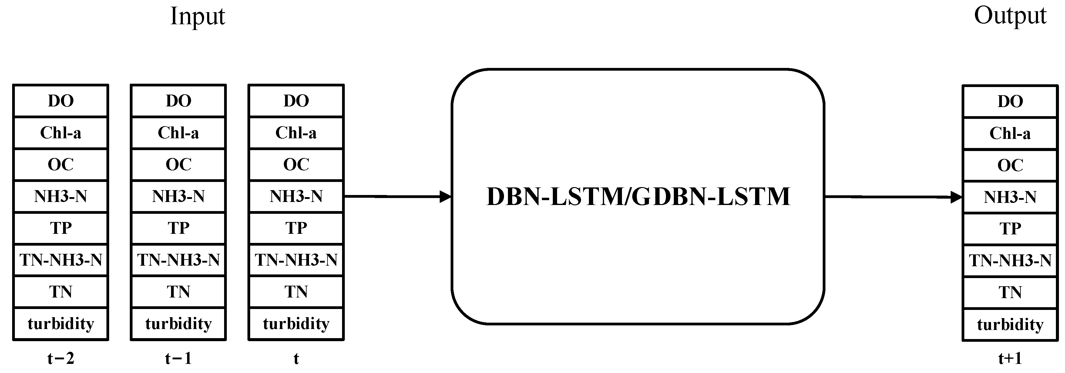
In the experiment, eight variables measured in the first three days, including a total of 24 water quality characteristics, were taken as model input, and eight variables on the next day were taken as model output. There were 1355 sets of input and output data. The input–output diagram of the proposed model is shown in Figure 7.
The first 80% of the data were used as training data, and the remaining 20% of the data were used as test data. Among them, the training set is divided into four parts for cross-verification to obtain the optimal hyperparameters. First, the training data were input into the GDBN network for pre-training. Networks with two, three, and four layers were set up. Finally, the GDBN network had three hidden layers throughout the experiment, which performed best on verification sets; the three hidden layers were regarded as three RBMSs for Gibbs sampling. The bottom layer denoted the visible layer, and the top layer was the hidden layer. Unsupervised training was performed to obtain the weights between the GDBN layers. Other hyperparameter settings that perform best on the validation set are obtained through experiments, too. The resulting parameters for the best performance of the revalidation set are as follows: The first layer had 48 neurons, the second layer consisted of 96 neurons, and the third layer had 24 neurons. The number of training epochs was 200. The activation function of the hidden layer was the ReLU function. The LSTM network had 64 neurons, which was defined using the output data dimension, and used the dropout layer to prevent overfitting with a drop probability of 0.2. The training set was constructed using the small batch gradient descent method, and the batch size was 32. Then, the gradient of each group was evaluated, and the model parameters were updated. The loss function was the mean square error (MSE). The number of iterations of the GDBN-LSTM network was 100.
To verify the feasibility and prediction effect of the proposed GDBN-LSTM model, the LSTM model, DBN model, DBN-LSTM model, and Convolutional Neural Network (CNN) model were used as comparison models in the experiment to predict the contents of DO, Chl-a, OC, NH3-N, TP, TN-NH3-N, TN, and turbidity. In these networks, the grid search method and cross-validation method are used to determine hyperparameters. Among them, the CNN convolutional layer contains 32 convolution kernels with the size of 3 × 3, which are filled with zero, and the activation function uses the ReLU function. The size of the pooled layer kernels is 2 × 2, and the step size is 2, to realize subsampling. The LSTM has three layers, the first with 100 neurons, the second with 50 neurons, and the third with 25 neurons, each with dropout layers that drop neurons with a probability of 0.2. The DBN has three layers, the first layer has 48 neurons, the second layer has 96 neurons, and the third layer has 24 neurons. The parameters of the DBN-LSTM network are the same as those of the GDBN-LSTM network.

4.1.3. Experimental Results Analysis

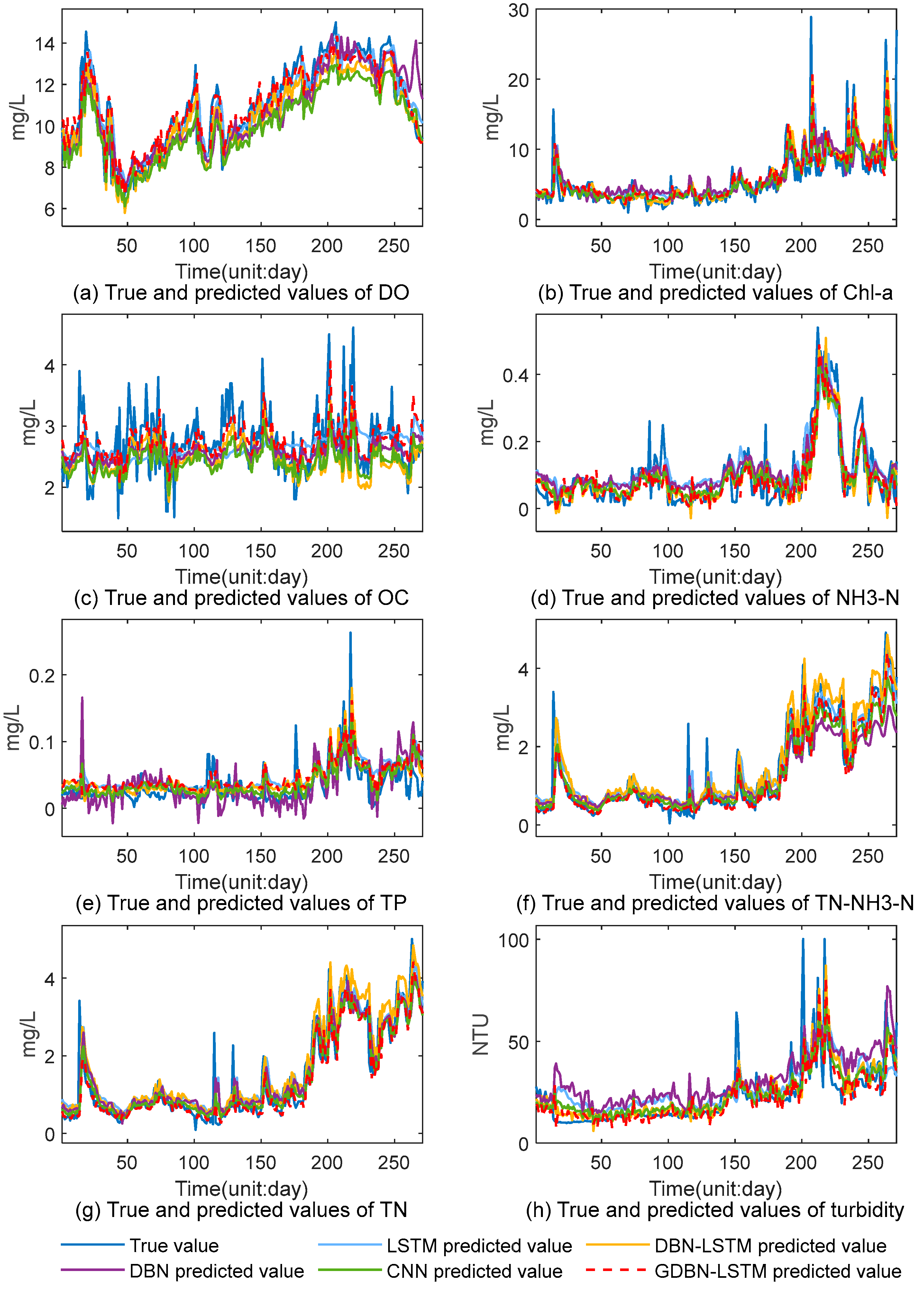
The comparison results of the five models on the test set are shown in Figure 8, where the dark-blue line represents the true value, the yellow line represents the predicted value of DBN-LSTM, the green line represents the predicted value of CNN, the light-blue line represents the predicted value of LSTM, the purple line represents the predicted value of DBN, and the red dashed line represents the predicted value of GDBN-LSTM.
As can be seen from Figure 8, the predicted results of the five models indicated that these models achieved a good fit between the real and predicted values. Furthermore, the prediction results of the DBN-LSTM model and GDBN-LSTM model were evidently better than those of the single LSTM model and DBN model in all water quality parameters, which indicated that DBN has the ability to extract data features, and can gradually abstract data features through multi-layer learning, and each layer can learn higher-level abstract features from the original data, thus helping to better characterize the data and lay the foundation for further processing. In order to better analyze the conclusion, the statistical results of the five models regarding different evaluation indicators are presented in Table 3.
As shown in Table 3, it is clear that the proposed algorithm GDBN-LSTM performed best in all variables. GDBN-LSTM results are superior to DBN-LSTM because GDBN has some advantages over DBN in processing continuous numerical data. DBN uses binary random variables, while GDBN uses Gaussian distribution to model data, so it is more suitable for continuous numerical data. This feature can better capture the correlation and distribution between continuous data, which makes for a better performance in prediction problems. GDBN-LSTM is also superior to the CNN network, because, on the basis of extracting data features, LSTM has advantages in processing time-series data, can more accurately capture the relationship between the past and the future, and has a good advantage in such prediction problems. Although the proposed algorithm has more advantages than other network results, some values are still low in multivariate water quality parameter prediction, such as Chl-a, OC, and TP. This is because in multivariate prediction, there may be different degrees of correlation between different variables. Some variables may have a stronger association with the target variable, making it easier to make accurate predictions, while others may have a lower correlation with the target variable, leading to less accurate predictions. The data quality of different variables may vary. Some variables may have more complete and accurate data, while others may have missing values, outliers, or noise, all of which can affect the predicted results. In a machine learning model, some variables may have a greater impact on the output of the model, which is called different feature importance. The model is more inclined to predict some features, while the prediction ability of other features is relatively weak.

4.1.4. Water Quality Evaluation Experiment

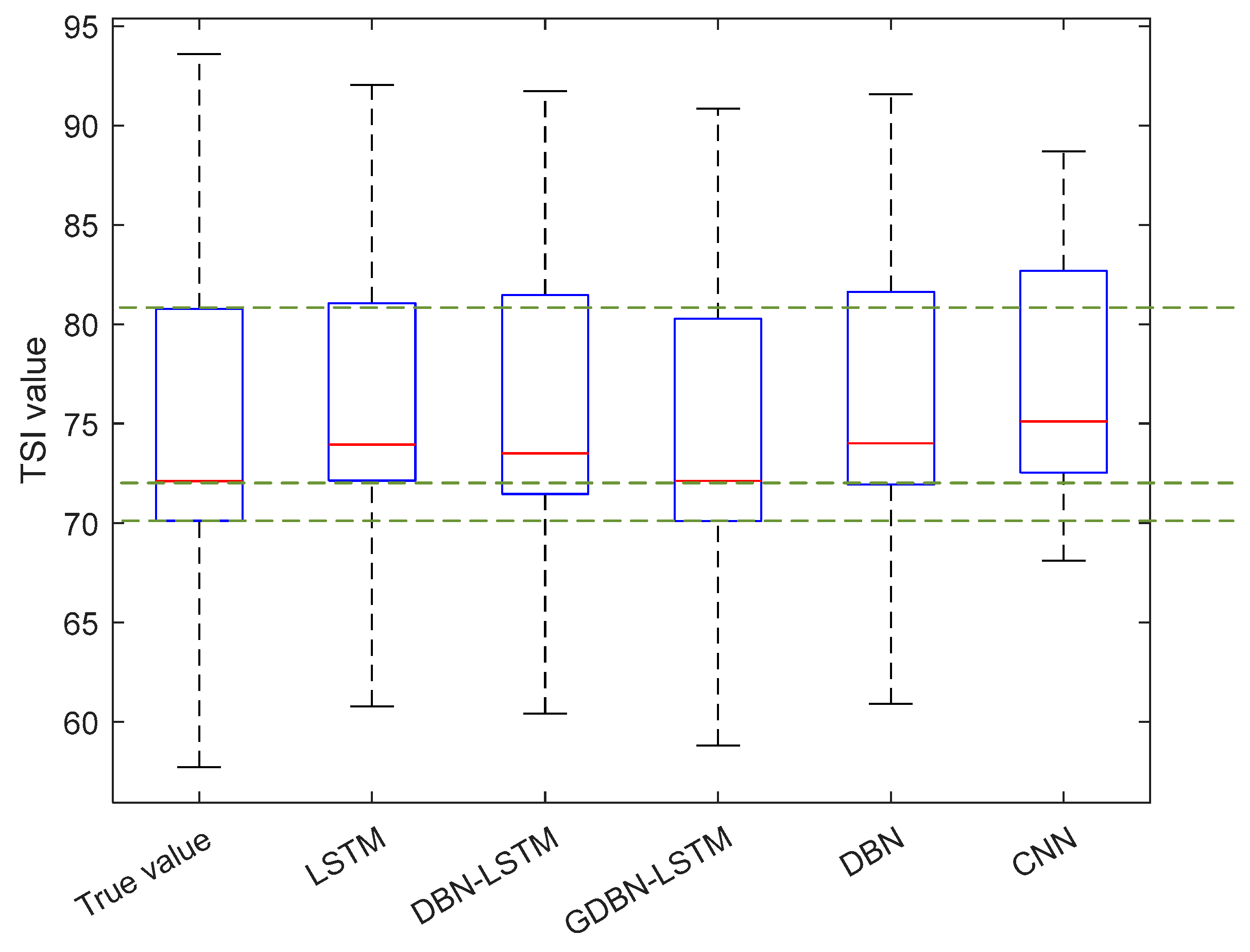
In this experiment, the TSI method was used to evaluate the water quality. Four indices, including Chl-a, TP, TN, and SD, were used to evaluate the water quality predicted via the LSTM, DBN, DBN-LSTM, GDBN-LSTM, and CNN models according to the above formulas (27)–(32). The box diagram of the TSI value distribution is shown in Figure 9.
The red line in the middle of the boxplot represents the median of the data, and the boxes at both ends of the boxplot represent the upper and lower quartiles of the data. They can show the distribution of the data. The length of the box can be used to measure the variation of the data. The boxplot in Figure 9 shows that compared to the four models, the GDBN-LSTM model could predict the water quality better, and its value range of digit and TSI were closer to the real values. The SMAPE, MAE, RMSE, and R 2 were used to evaluate the TSI calculated using the predicted values of the five networks. The statistical results are shown in Table 4:
As shown in Table 4, the SMAPE, MAE, and RMSE values of the GDBN-LSTM model were all lower than those of other models, while the R 2 value of the GDBN-LSTM model was higher than that of other models; thus, the error rate and fitting degree of the GDBN-LSTM were better than those of other networks. Therefore, the water quality prediction result of the DBN-LSTM model was closer to the real value than that of other models. Among them, the fitting degree of GDBN-LSTM is as high as 0.9. Compared with the fitting degree predicted using other water quality parameters in Table 3, the calculated TSI has a better fitting degree, which indicates the processing ability of the proposed network for important data.
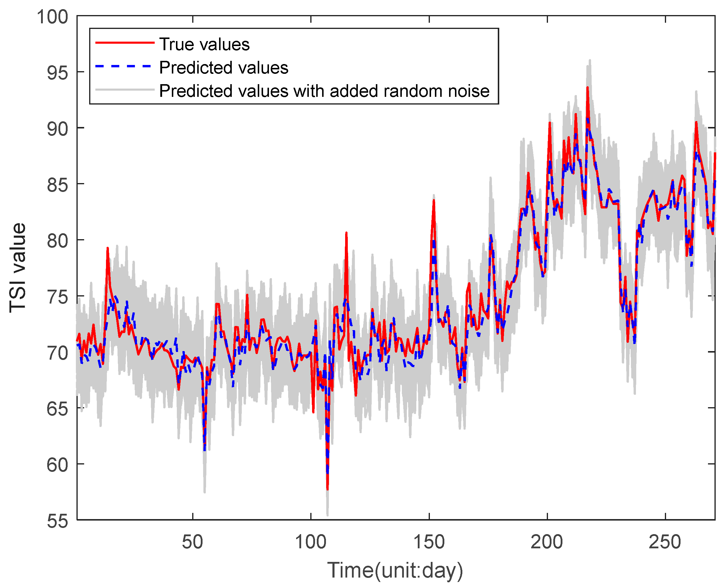
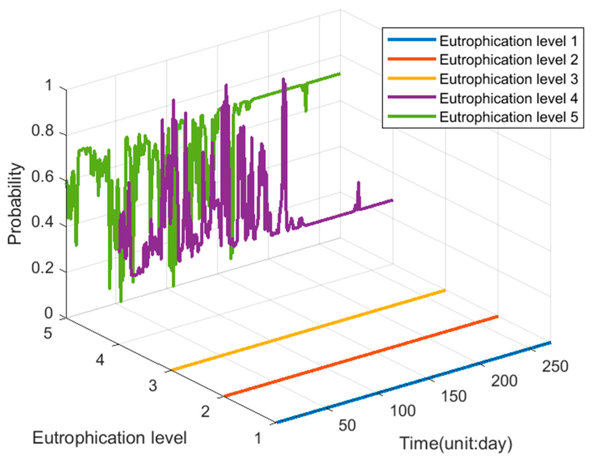
Since the TSI calculated using the predicted value is a single-value water quality assessment, if the prediction is inaccurate, the result will be greatly affected. To better evaluate the future water quality based on the predicted values, random noise was added to the predicted values according to GDBN-LSTM and fitted 100 times, where MSE is the standard deviation. This can predict the probability of a certain level of water quality in the future. As shown in Figure 10, it indicated that the true value is basically within the predicted range, and the probability of future water quality grade was calculated based on the data fitted 100 times. The red line represents the true value, the blue dashed line represents the predicted value, and the gray interval represents the range between 100 fits. It indicated that the true value was basically within the predicted range, and the probability of future water quality grade is calculated based on the data fitted 100 times. As shown in Figure 11 and Figure 12, which clearly demonstrate the probability of future water quality occurring at that level where the blue line represents eutrophication level 1, the red line represents eutrophication level 2, the yellow line represents eutrophication level 3, the purple line represents eutrophication level 4, and the green line represents eutrophication level 5. Figure 12 shows the probability of water quality being at each eutrophication level in the future over time. The water quality grade is basically in the range of 4~5, where the water quality is the most serious around July, followed by a period of decline in August, and a rise to serious levels again.

4.2. Univariable Timing Prediction and Evaluation

4.2.1. Data Selection and Preprocessing

The water quality data of three stores in Beijing were predicted using the DO value for a one-step time series, and its content on the next day was predicted using the historical data on DO collected on the previous three days. The same normalization method was adopted as in Section 4.1.

4.2.2. Experimental Parameter Settings

The experimental configuration was the same as that in Section 4.1 through cross-validation, and the only difference was that the number of neurons in the first, second, and third GDBN layers in this experiment was 10, 20, and 3, respectively. The input and output of the proposed model are shown in Figure 13.
The small batch gradient descent method was employed in the experiment, and the MSE was used as a loss function. The number of iterations of the training process is 100.
To verify the feasibility and prediction effect of the proposed GDBN-LSTM model, the LSTM model, DBN model, DBN-LSTM model, and Convolutional Neural Network (CNN) model were used as comparison models in the experiment to predict the content of DO, Chl-a, OC, NH3-N, TP, TN-NH3-N, TN, and turbidity. In these networks, the grid search method and cross-validation method were used to determine hyperparameters. Among them, the CNN convolutional layer contains 32 convolution kernels with the size of 3×1, which are filled with zero, and the activation function uses the ReLU function. The LSTM has three layers, the first with 100 neurons, the second with 50 neurons, and the third with 25 neurons, each with dropout layers that drop neurons with a probability of 0.2. The DBN has three layers, the first layer has 10 neurons, the second layer has 20 neurons, and the third layer has 3 neurons. The parameters of the DBN-LSTM network are the same as those of the GDBN-LSTM network.

4.2.3. Experimental Results Analysis

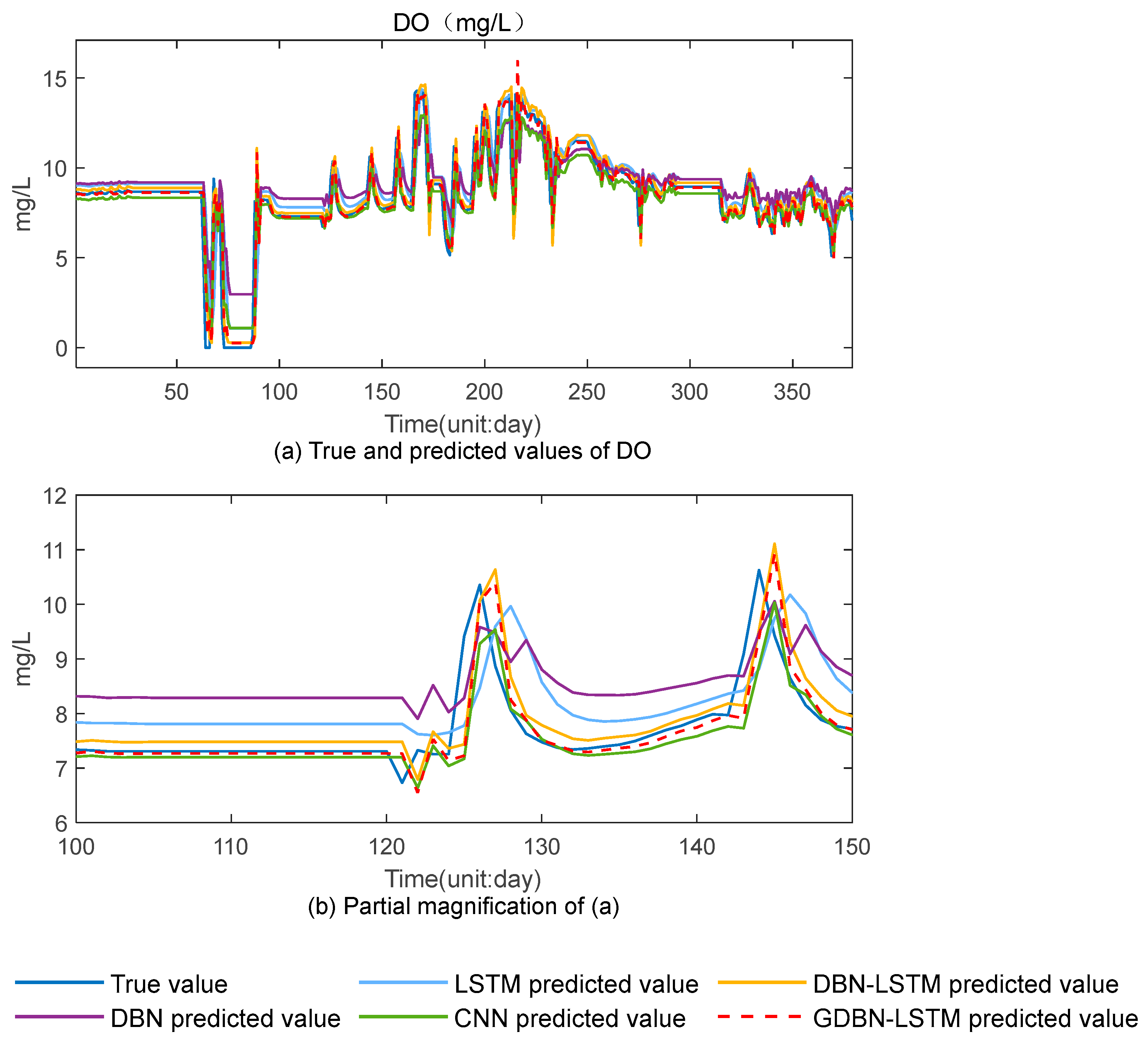
In the experiment, the predicted value of DO obtained using the proposed GDBN-LSTM model was compared with that predicted using the LSTM model, DBN model DBN-LSTM model, and CNN model, as shown in Figure 14. It was clear that the DBN-LSTM model and the GDBN-LSTM model have better predicted results, which indicated the ability and importance of DBN to extract data features.
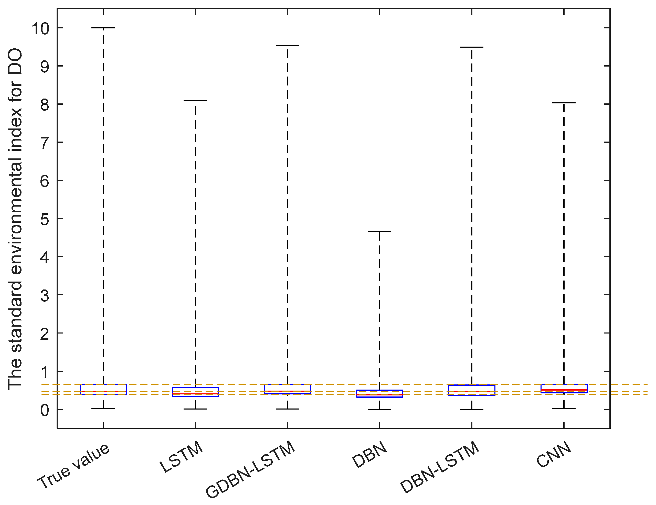
To compare the various networks more intuitively, the statistical results of the five models regarding different evaluation indicators are shown in Table 5; The MAE, RMSE, and SMAPE of the GDBN-LSTM model were lower than those of the LSTM model, DBN-LSTM model, DBN model, and CNN model and the R 2 were higher than those of the LSTM model, DBN-LSTM model, DBN model, and CNN model. Combined with Figure 15, it indicated that GDBN-LSTM had a good ability to predict the amount of mutation, which indicated that GDBN played a better role than DBN in the feature extraction and denoising factors affecting water quality. The experimental results demonstrated the high accuracy of the proposed GDBN-LSTM in water quality prediction.

4.2.4. Water Quality Evaluation Experiment

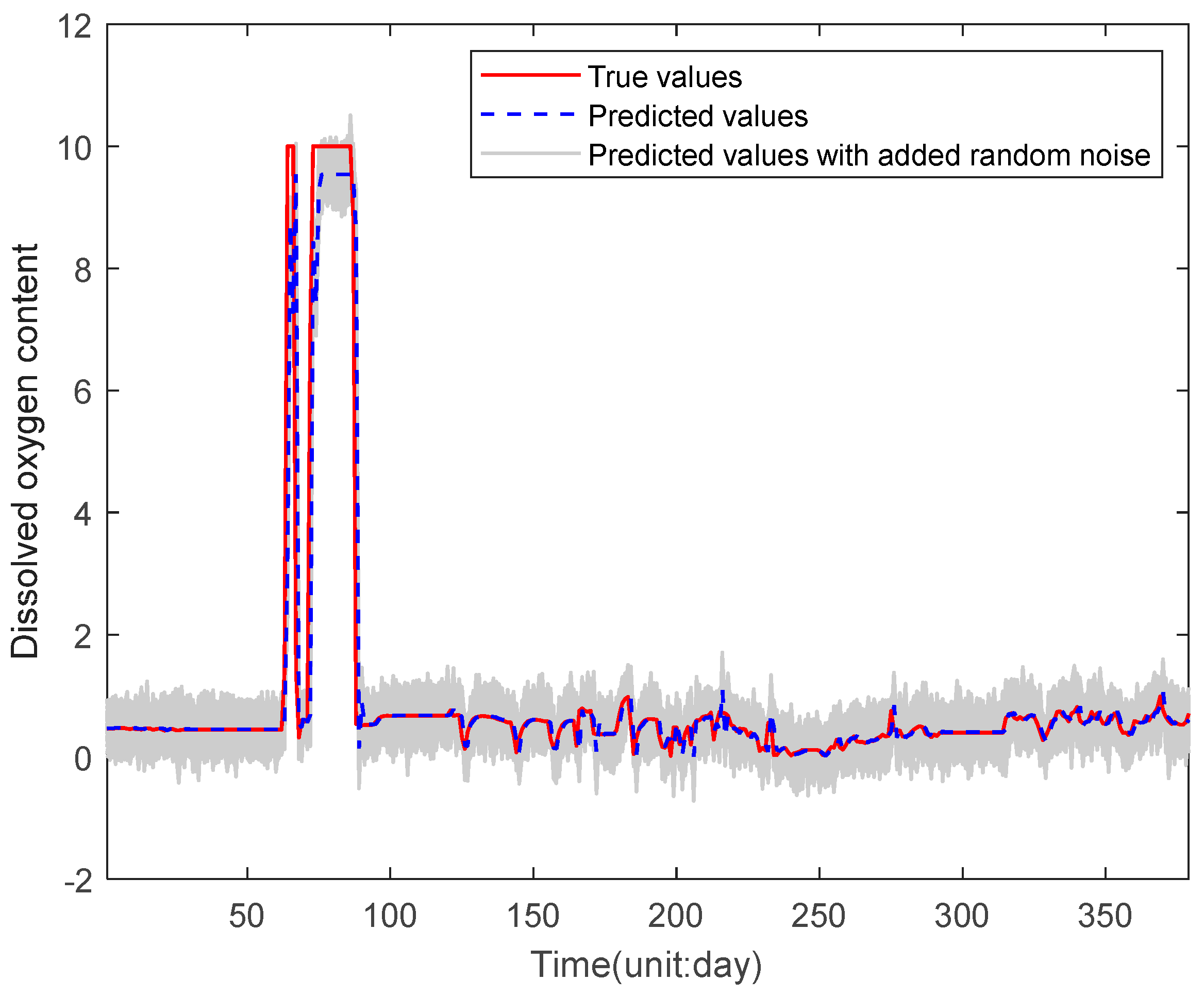
Based on the prediction, this experiment adopted the single-factor index evaluation method and used the DO data to calculate the environmental index to judge the water pollution level. The evaluation standard was the third type of water quality. The evaluation results are shown in Figure 15.
As shown in Figure 15, the GDBN-LSTM predicts that the maximum, median, upper, and lower quartile values of water quality were close to the real values, once again showing that GDBN had better predictability for mutated data, and its median was also the closest to the real value, which again indicated the accuracy of water quality and evaluation based on GDBN-LSTM prediction. The SMAPE, MAE, RMSE, and R 2 indicators were used to evaluate the nutritional indices calculated from the predicted values of the four networks, and the statistical results are shown in Table 6.
As shown in Table 6, the GDBN-LSTM network had a better fitting rate and accuracy than other networks in the single-factor water quality assessment. This result indicated that the GDBN-LSTM had more advantages than other networks in water quality assessment.
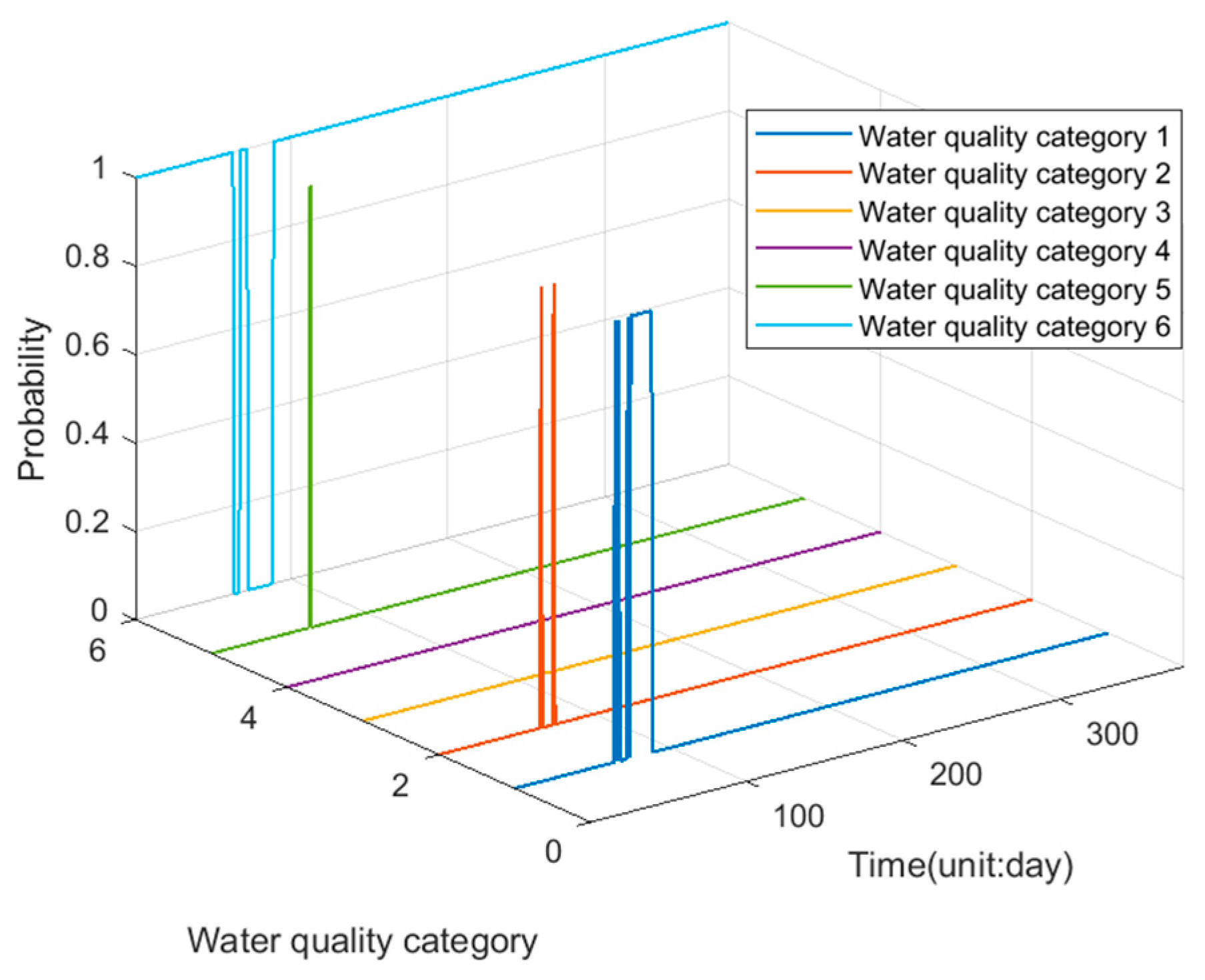
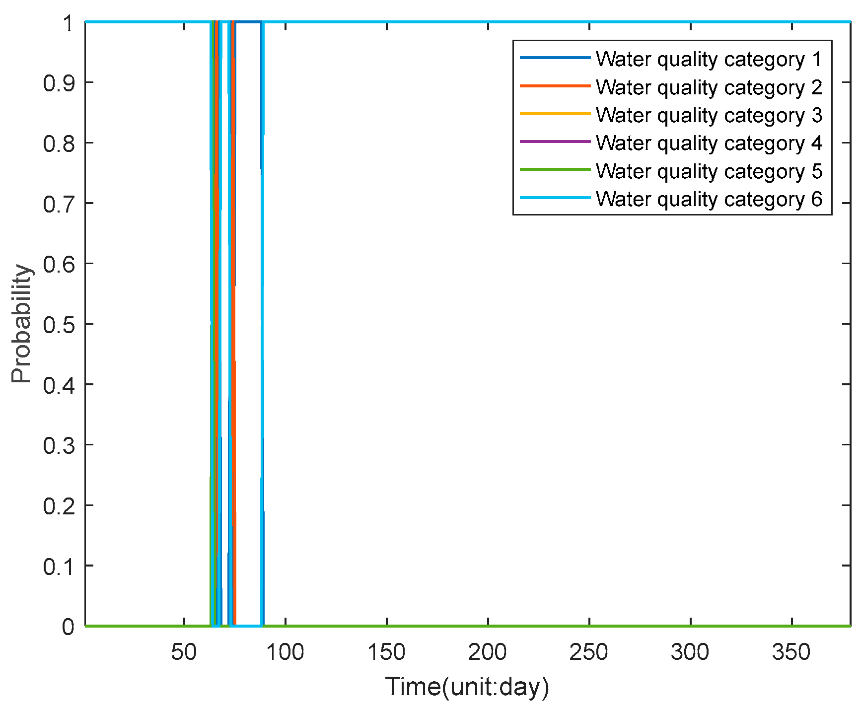
Also, for a better evaluation of water quality to make decisions, the same treatment was conducted as in Section 4.1. In the GDBN-LSTM predicted data plus random noise, evolved 100 times, noise instead of prediction error, it was seen that the true value was mostly included in the range, as shown in Figure 16. Then, the probability that the water quality is at grade based on the evolved values is calculated, as shown in Figure 17 and Figure 18, where the blue line represents eutrophication level 1, the red line represents eutrophication level 2, the yellow line represents eutrophication level 3, the purple line represents eutrophication level 4, and the green line represents eutrophication level 5. Figure 18 shows the probability of water quality being at each eutrophication level in the future over time.
Figure 17 and Figure 18 indicated that the water quality had the highest probability of being at level 5 in the future period, which requires the relevant departments to introduce appropriate treatment programs to protect the environment.

5. Conclusions

The GDBN-LSTM prediction model developed in this paper can be trained on different water quality data and has a wide range of application scenarios. The experimental results show that the proposed neural network model can predict water quality well, and the GDBN with GRBM stacking improves the data feature loss caused by the classical RBM stacking DBN visible layer and hidden layer duality problem, which is then input to the LSTM network, providing a new and feasible way for water quality prediction. In this paper, the single-factor indicator evaluation method and TSL are used to evaluate water quality, the prediction results of the proposed network and other networks are compared with different evaluation indicators, and the experimental results show that the proposed network has a higher evaluation accuracy. After that, the probabilities of future water quality categories are obtained by adding random noise for multiple evolutions, which provides a new idea for future water pollution prevention and control. Some limitations should be noted. First, the model is only conducted based on a specific water quality data set, and its generalization ability needs to be further verified. Second, dealing with anomalies or long-term data changes has not been explored in-depth, and more research is needed on how models perform under extreme conditions. Finally, due to the limitations of input data quality and sampling frequency in practical applications, further optimization may be required for application scenarios with high real-time requirements. This study is based on data-driven water quality prediction. In the future, water quality prediction should be combined with a water quality mechanism model, and uncertainty should be added to the prediction to assess future water quality more accurately.

Author Contributions

Writing—original draft, B.F.; Writing—review & editing, Z.Z.; Visualization, Y.Z. All authors have read and agreed to the published version of the manuscript.

Funding

This work was supported in part by the Beijing Natural Science Foundation under Grant 4222042, and in part by the National Key R&D Program of China under Grant 2022YFF1101103.

Data Availability Statement

The data presented in this study are available on request from the corresponding author.

Conflicts of Interest

The authors declare no conflicts of interest.

References

  1. Zhang, X.J.; Chen, C.; Lin, P.F.; Hou, A.X.; Niu, Z.B.; Wang, J. Emergency drinking water treatment during source water pollution accidents in China: Origin analysis, framework and technologies. Environ. Sci. Technol. 2011, 45, 161–167. [Google Scholar] [CrossRef] [PubMed]
  2. Loi, J.X.; Chua, A.S.; Rabuni, M.F.; Tan, C.K.; Lai, S.H.; Takemura, Y.; Syutsubo, K. Water quality assessment and pollution threat to safe water supply for three river basins in Malaysia. Sci. Total Environ. 2022, 832, 155067. [Google Scholar] [CrossRef] [PubMed]
  3. Zhang, J.; Zhang, Y.; Sun, G.; Song, C.; Li, J.; Hao, L.; Liu, N. Climate Variability Masked Greening Effects on Water Yield in the Yangtze River Basin during 2001–2018. Water Resour. Res. 2022, 58, e2021WR030382. [Google Scholar] [CrossRef]
  4. Bedri, Z.; Corkery, A.; O’Sullivan, J.J.; Deering, L.A.; Demeter, K.; Meijer, W.G.; O’Hare, G.; Masterson, B. Evaluating a microbial water quality prediction model for beach management under the revised EU Bathing Water Directive. J. Environ. Manag. 2016, 167, 49–58. [Google Scholar] [CrossRef] [PubMed]
  5. Lin, S.S.; Shen, S.L.; Zhou, A.; Lyu, H.M. Assessment and management of lake eutrophication: A case study in Lake Erhai, China. Sci. Total Environ. 2020, 751, 141618. [Google Scholar] [CrossRef] [PubMed]
  6. Wang, X.; Zhou, Y.; Zhao, Z.; Wang, L.; Xu, J.; Yu, J. A novel water quality mechanism modeling and eutrophication risk assessment method of lakes and reservoirs. Nonlinear Dyn. 2019, 96, 1037–1053. [Google Scholar] [CrossRef]
  7. Zhao, L. Prediction momel of ecological environmental water demand based on big data analysis. Environ. Technol. Innov. 2021, 21, 101196. [Google Scholar] [CrossRef]
  8. Bai, J.; Zhao, J.; Zhang, Z.; Tian, Z. Assessment and a review of research on surface water quality modeling. Ecol. Model. 2022, 466, 109888. [Google Scholar] [CrossRef]
  9. Xiong, H.; Liu, T.; Wang, H.; Feng, C. Simulation of the improving effect of graphene visible-light photocatalysis using the MIKE11 model of an urban landscape river in the Chaohu Lake Basin, China. Nat. Resour. Model. 2022, 35, e12344. [Google Scholar] [CrossRef]
  10. Chen, C.F.; Chong, K.Y.; Lin, J.Y. A combined catchment-reservoir water quality model to guide catchment management for reservoir water quality control. Water. Environ. J. 2021, 35, 1025–1037. [Google Scholar] [CrossRef]
  11. Valikhan Anaraki, M.; Mahmoudian, F.; Nabizadeh Chianeh, F.; Farzin, S. Dye Pollutant Removal from Synthetic Wastewater: A New Modeling and Predicting Approach Based on Experimental Data Analysis, Kriging Interpolation Method, and Computational Intelligence Techniques. J. Environ. Inform. 2022, 40, 84. [Google Scholar] [CrossRef]
  12. Shabani, A.; Zhang, X.; Chu, X.; Zheng, H. Automatic Calibration for CE-QUAL-W2 Model Using Improved Global-Best Harmony Search Algorithm. Water 2021, 13, 2308. [Google Scholar] [CrossRef]
  13. Jin, T.; Cai, S.; Jiang, D.; Liu, J. A data-driven model for real-time water quality prediction and early warning by an integration method. Environ. Sci. Pollut. Res. 2019, 26, 30374–30385. [Google Scholar] [CrossRef] [PubMed]
  14. Meng, X.; Zhang, Y.; Qiao, J. An adaptive task-oriented RBF network for key water quality parameters prediction in wastewater treatment process. Neural Comput. Appl. 2021, 33, 11401–11414. [Google Scholar] [CrossRef]
  15. Zhao, Z.; Zhou, Y.; Wang, X.; Wang, Z.; Bai, Y. Water quality evolution mechanism modeling and health risk assessment based on stochastic hybrid dynamic systems. Expert Syst. Appl. 2022, 193, 116404. [Google Scholar] [CrossRef]
  16. Uddin, M.G.; Nash, S.; Olbert, A.I. A review of water quality index models and their use for assessing surface water quality. Ecol. Indic. 2021, 122, 107218. [Google Scholar] [CrossRef]
  17. Wu, Z.; Zhang, D.; Cai, Y.; Wang, X.; Zhang, L.; Chen, Y. Water quality assessment based on the water quality index method in Lake Poyang: The largest freshwater lake in China. Sci. Rep. 2017, 7, 17999. [Google Scholar] [CrossRef] [PubMed]
  18. Kumari, R.; Sharma, R.C. Assessment of water quality index and multivariate analysis of high altitude sacred Lake Prashar, Himachal Pradesh, India. Int. J. Environ. Sci. Technol. 2018, 16, 6125–6134. [Google Scholar] [CrossRef]
  19. Yan, F.; Liu, L.; Li, Y.; Zhang, Y.; Chen, M.; Xing, X. A dynamic water quality index model based on functional data analysis. Ecol. Indic. 2020, 32, 544–552. [Google Scholar] [CrossRef]
  20. Ahsan, W.A.; Ahmad, H.R.; Farooqi, Z.U.; Sabir, M.; Ayub, M.A.; Rizwan, M.; Ilic, P. Surface water quality assessment of Skardu springs using Water Quality Index. Environ. Sci. Pollut. Res. 2021, 28, 20537–20548. [Google Scholar] [CrossRef]
  21. Yotova, G.; Varbanov, M.; Tcherkezova, E.; Tsakovski, S. Water quality assessment of a river catchment by the composite water quality index and self-organizing maps. Ecol. Indic. 2015, 57, 249–258. [Google Scholar] [CrossRef]
  22. Lizotte, R.E., Jr.; Yasarer, L.M.; Bingner, R.L.; Locke, M.A.; Knight, S.S. Long-Term Oxbow Lake Trophic State under Agricultural Best Management Practices. Water 2021, 13, 1123. [Google Scholar] [CrossRef]
  23. Bomfim, E.D.; Kraus, C.N.; Lobo, M.T.; Nogueira, I.D.; Peres, L.G.; Boaventura, G.R.; Laques, A.E.; Garnier, J.; Seyler, P.; Marques, D.M.; et al. Trophic state index validation based on the phytoplankton functional group approach in Amazon floodplain lakes. Inland Waters 2019, 9, 309–319. [Google Scholar] [CrossRef]
  24. Markad, A.T.; Landge, A.T.; Nayak, B.B.; Inamdar, A.B.; Mishra, A.K. Trophic state modeling for shallow freshwater reservoir: A new approach. Environ. Monit. Assess. 2019, 191, 586. [Google Scholar] [CrossRef] [PubMed]
  25. Yang, L.-K.; Peng, S.; Zhao, X.-H.; Li, X. Development of a two-dimensional eutrophication model in an urban lake (China) and the application of uncertainty analysis. Ecol. Model. 2017, 345, 63–74. [Google Scholar]
  26. Khozani, Z.S.; Banadkooki, F.B.; Ehteram, M.; Ahmed, A.N.; El-Shafie, A. Combining autoregressive integrated moving average with Long Short-Term Memory neural network and optimisation algorithms for predicting ground water level. J. Clean. Prod. 2022, 348, 131224. [Google Scholar] [CrossRef]
  27. Liu, P.; Wang, J.; Sangaiah, A.K.; Xie, Y.; Yin, X. Analysis and Prediction of Water Quality Using LSTM Deep Neural Networks in IoT Environment. Sustainability 2019, 11, 2058. [Google Scholar] [CrossRef]
  28. Zou, M.; Conzen, S.D. A new dynamic Bayesian network (DBN) approach for identifying gene regulatory networks from time course microarray data. Bioinformatics 2005, 21, 71–79. [Google Scholar] [CrossRef]
  29. Yan, J.; Gao, Y.; Yu, Y.; Xu, H.; Xu, Z. A Prediction Model Based on Deep Belief Network and Least Squares SVR Applied to Cross-Section Water Quality. Water 2020, 12, 1929. [Google Scholar] [CrossRef]
  30. Xie, G.S.; Jin, X.B.; Zhang, X.Y.; Zang, S.F.; Yang, C.; Wang, Z.; Pu, J. From Class-Specific to Class-Mixture: Cascaded Feature Representations via Restricted Boltzmann Machine Learning. IEEE Access 2018, 6, 69393–69406. [Google Scholar] [CrossRef]
  31. Hinton, G.E.; Salakhutdinov, R.R. Reducing the dimensionality of data with neural networks. Science 2006, 313, 504–507. [Google Scholar] [CrossRef]
  32. Imneisi, I.; Aydin, M. Water quality assessment for Elmali stream and Karaomak stream using the comprehensive pollution index (CPI) in Karaomak watershed, Kastamonu, Turkey. Fresenius Environ. Bull. 2018, 27, 7031–7038. [Google Scholar]
  33. Carlson, R. A Trophic State Index for Lakes. Limnol. Oceanogr. Methods 1977, 22, 361–369. [Google Scholar] [CrossRef]
  34. Bilgin, A. Trophic state and limiting nutrient evaluations using trophic state/level index methods: A case study of Borka Dam Lake. Environ. Monit. Assess. 2020, 192, 794. [Google Scholar] [CrossRef] [PubMed]
  35. Wu, J.; Wang, Z. A Hybrid Model for Water Quality Prediction Based on an Artificial Neural Network, Wavelet Transform, and Long Short-Term Memory. Water 2022, 14, 610. [Google Scholar] [CrossRef]
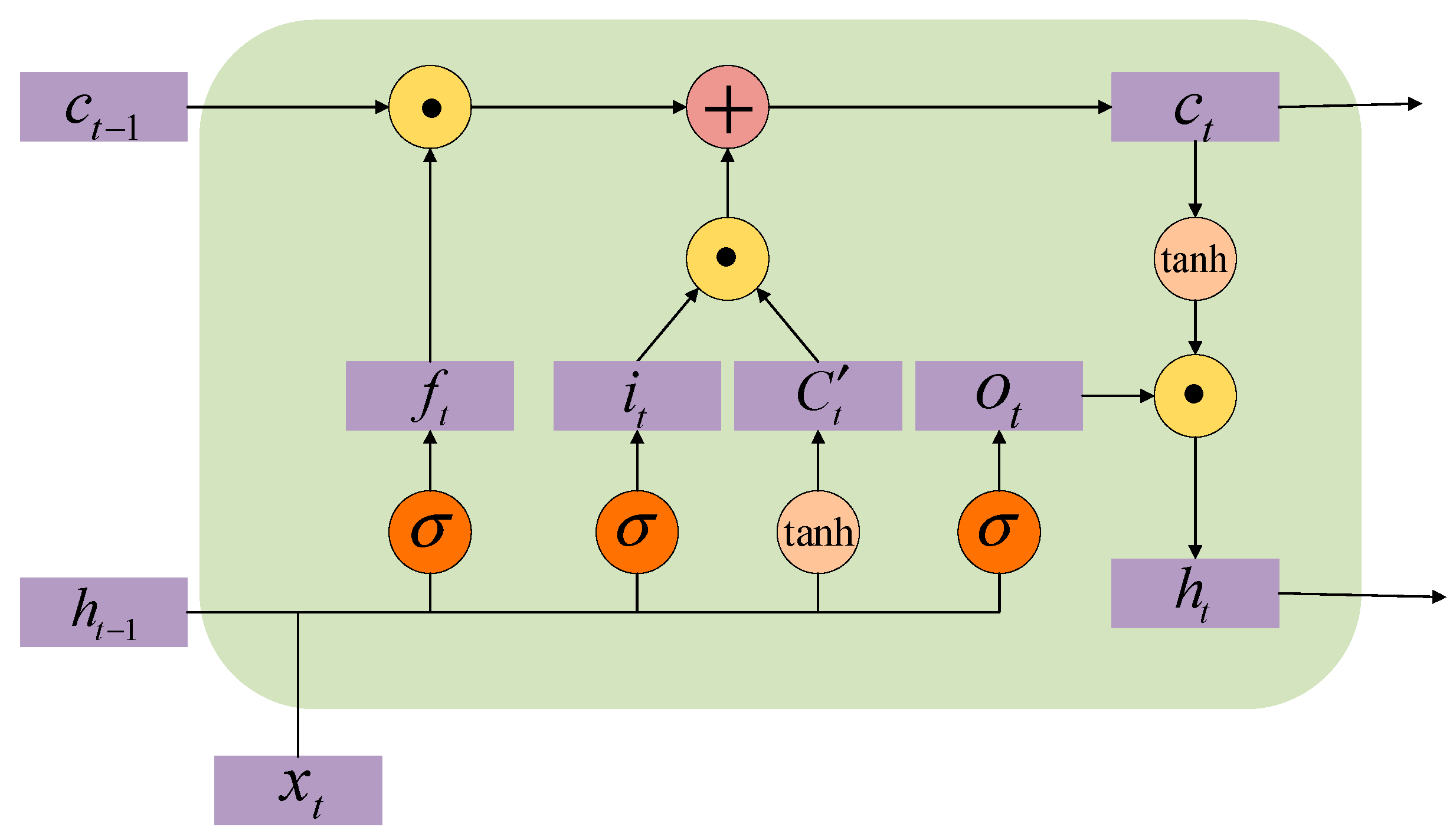
Figure 1. The LSTM structure.
Water 16 01362 g001
Figure 2. The simplified structure of a deep confidence network consisting of three layers.
Water 16 01362 g002
Figure 3. The layer-by-layer pre-training process.
Water 16 01362 g003
Figure 4. Illustration of the fine-tuning process.
Water 16 01362 g004
Figure 5. The structure of the proposed prediction network model.
Water 16 01362 g005
Figure 6. The flowchart of the proposed GDBN-LSTM algorithm.
Water 16 01362 g006
Figure 7. The input–output diagram of the proposed model.
Water 16 01362 g007
Figure 8. Comparison results of the LSTM and DBN-LSTM models on the test set.
Water 16 01362 g008
Figure 9. The box diagram of the TSI value distribution.
Water 16 01362 g009
Figure 10. TSI predicted value range compared with the true values.
Water 16 01362 g010
Figure 11. Probability 3D map of future water quality grade.
Water 16 01362 g011
Figure 12. Probability 2D map of future water quality grade.
Water 16 01362 g012
Figure 13. The input–output diagram of the proposed model in the experiment.
Water 16 01362 g013
Figure 14. The comparison results of the DO prediction by four models.
Water 16 01362 g014
Figure 15. Box line diagram of five network single-factor evaluation methods.
Water 16 01362 g015
Figure 16. The single-factor index-predicted value range compared with the true values.
Water 16 01362 g016
Figure 17. Probability 3D map of future water quality grade.
Water 16 01362 g017
Figure 18. Probability 2D map of future water quality grade.
Water 16 01362 g018
Table 1. Water quality evaluation criteria based on the DO content.
Water Quality CategoryDO Content
(mg/L)
I7.5
II6
III5
IV3
V2
Table 2. The TSI classification.
TSI
SD
(m)
TP
(μg P/L)
Chl-a
(μg/L)
TN
(mg N/L)
Ultraoligotrophic 0 64 0.75 0.04 0.02
Ultraoligotrophic 10 32 1.5 0.12 0.05
Ultraoligotrophic 20 16 3 0.34 0.09
Oligotrophic 30 8 6 0.94 0.18
Oligotrophic 40 4 12 2.6 0.37
Mesotrophic 45 2.8 17 5 0.52
Mesotrophic 50 2 24 6.4 0.74
Eutrophic 53 1.6 30 10 0.92
Eutrophic 60 1 48 20 1.47
Hypereutrophic 70 0.5 96 56 2.94
Hypereutrophic 80 0.25 192 154 5.89
Hypereutrophic 90 0.12 384 427 11.7
Hypereutrophic 100 0.062 768 1183 23.6
Table 3. The statistical results of the different network indicators of the five models.
SMAPERMSEMAE R 2
DO (mg/L) LSTM0.0429 0.9105 0.6716 0.8102
DBN0.0550 1.1395 0.8816 0.7028
DBN-LSTM0.0415 0.8523 0.6720 0.8337
CNN0.0605 1.1687 0.9943 0.6874
GDBN-LSTM0.0329 0.7196 0.5105 0.8815
Chl-a (mg/L) LSTM0.1826 2.9331 1.6166 0.4254
DBN0.1939 2.9282 1.6808 0.4273
DBN-LSTM0.1570 2.8669 1.5746 0.4511
CNN0.1451 2.8392 1.4729 0.4589
GDBN-LSTM0.1319 2.7544 1.3509 0.4958
OC (mg/L) LSTM0.0932 0.5020 0.3810 0.1979
DBN0.0839 0.4632 0.3455 0.1652
DBN-LSTM0.0931 0.5006 0.3792 0.1919
CNN0.0972 0.5204 0.3996 0.1599
GDBN-LSTM0.0791 0.4403 0.3212 0.3554
NH3-N (mg/L) LSTM0.4857 0.0641 0.0517 0.6455
DBN0.4516 0.0571 0.0455 0.7191
DBN-LSTM0.3828 0.0546 0.0389 0.7429
CNN0.3694 0.0543 0.0390 0.7454
GDBN-LSTM0.3578 0.0539 0.0381 0.7491
TP (mg/L) LSTM0.4077 0.0263 0.0198 0.2924
DBN0.4480 0.0303 0.0205 0.2078
DBN-LSTM0.3389 0.0240 0.0163 0.2475
CNN0.3013 0.0230 0.0185 0.3073
GDBN-LSTM0.2886 0.0202 0.0145 0.4702
TN-NH3-N (mg/L) LSTM0.2250 0.4793 0.3358 0.8228
DBN0.1976 0.5598 0.3610 0.7581
DBN-LSTM0.2200 0.4796 0.3578 0.8225
CNN0.1471 0.4378 0.2610 0.8521
GDBN-LSTM0.1297 0.4164 0.2278 0.8662
TN (mg/L) LSTM0.2243 0.4949 0.3581 0.8283
DBN0.1869 0.4560 0.3087 0.8542
DBN-LSTM0.2094 0.4808 0.3634 0.8379
CNN0.1389 0.4266 0.2508 0.8783
GDBN-LSTM0.1218 0.4127 0.2328 0.8747
Turbidity (NTU) LSTM0.2178 11.0218 7.7475 0.4289
DBN0.2894 12.5788 10.1933 0.2561
DBN-LSTM0.1375 9.2058 5.3354 0.6016
CNN0.1465 9.9364 5.3282 0.6245
GDBN-LSTM0.1391 9.2617 5.2647 0.6967
Table 4. Evaluation indices of the TSI accuracy of the five models.
SMAPEMAE R 2 RMSE
TSI valueLSTM2.32791.72070.89502.1064
DBN2.30121.69940.89352.1211
DBN-LSTM1.42601.06780.94901.4685
CNN3.36541.93390.77643.4011
GDBN-LSTM1.33911.00120.95431.3902
Table 5. Comparison of environmental index prediction results of the five models.
SMAPERMSEMAE R 2
DOLSTM0.16131.45650.92340.6839
DBN0.55141.40941.01030.7040
DBN-LSTM0.15631.25080.95200.7669
CNN0.10011.12280.74150.8016
GDBN-LSTM0.09491.12040.69620.8130
Table 6. Comparison of the environmental index prediction results of the five methods.
SMAPERMSEMAE R 2
LSTM0.24181.19830.34700.6592
DBN0.28321.48250.45280.4932
DBN-LSTM0.27710.80180.25270.8467
CNN0.19020.92510.22730.7936
GDBN-LSTM0.18210.79290.19630.8496
Disclaimer/Publisher’s Note: The statements, opinions and data contained in all publications are solely those of the individual author(s) and contributor(s) and not of MDPI and/or the editor(s). MDPI and/or the editor(s) disclaim responsibility for any injury to people or property resulting from any ideas, methods, instructions or products referred to in the content.