Deep Learning-Based Simulation of Surface Suspended Sediment Concentration in the Yangtze Estuary during Typhoon In-Fa

Abstract

Effectively simulating the variation in suspended sediment concentration (SSC) in estuaries during typhoons is significant for the water quality and ecological conditions of estuarine shoal wetlands and their adjacent coastal waters. During typhoons, SSC undergoes large variations due to the significant changes in meteorological and hydrological factors such as waves, wind speed, and precipitation, which increases the difficulty in simulating SSC. Therefore, in this study, we use an optimized Principal Component Analysis Long Short-Term Memory (PCA-LSTM) framework with an attention mechanism to simulate the SSC in the Yangtze Estuary during Typhoon In-Fa. First, we integrate data from different sources into a multi-source dataset. Second, we use the PCA to reduce the dimensionality of the multi-source data and eliminate redundant variables in the feature data. Third, we introduce an attention mechanism to optimize the long and short-term memory (LSTM) model. Finally, we use the differential evolution (DE) algorithm for hyperparameter selection and merge the feature data with the SSC data as the input of the optimized LSTM network to simulate SSC. The results showed that SSC’s fitting coefficients (R²) at four hydrological stations improved by 7.5%, 6.1%, 7.4%, and 7.8%, respectively, using the attention-based PCA-LSTM compared to the PCA-LSTM. Moreover, compared to the traditional LSTM model, the R² was improved by 33.8%, 30.5%, 32.0%, and 28.6%, respectively, using the attention-based PCA-LSTM framework. The study indicates that the selection of input variables can affect the model results. Introducing an attention mechanism can effectively optimize the PCA-LSTM framework and improve the simulation accuracy, which helps simulate the non-linear process of SSC variation occurring during Typhoon In-Fa.

1. Introduction

Suspended sediment concentration (SSC) is a crucial indicator of water quality. Its changes play a vital role in the water quality and ecology of coastal waters. They have an essential impact on bed erosion and sedimentation, primary biological productivity, and land resource protection [1]. As one of the most frequent natural phenomena in estuaries and adjacent coastal areas, typhoons significantly impact the SSC in estuaries and coastal areas [2,3]. In estuaries and coastal areas, typhoons can cause changes in seabed topography and coastal geomorphology, leading to tidal flat accumulation, erosion, and shoreline movement [3]. Therefore, monitoring and simulating SSC changes in estuary areas during typhoons is significant for ecological protection and aquatic and agricultural production [4].

With the development of artificial intelligence (AI) technology, deep learning has become more accurate and effective in predicting and simulating complex nonlinear data [5]. Advanced deep learning (DL) methods, such as long short-term memory (LSTM), enable algorithms consisting of multiple processing layers to discover underlying patterns in data [6,7,8,9,10]. In the field of hydrological modeling, Keivan Kaveh et al. [6] used the LSTM model to predict SSC, and the R² of the model output reached 0.8161, indicating that the LSTM model can predict SSC well. Previous studies have used the traditional LSTM model to predict and simulate SSC in calm weather. The traditional LSTM network can effectively extract the autoregressive dependencies of data, but it has poor processing ability for redundant data [5,11]. The LSTM model for simulating SSC changes during typhoons involves a large amount of high-dimensional and redundant data [12,13], which will affect the effect of LSTM models for simulating SSC changes during typhoons. Therefore, it is essential to reduce redundancy in feature data while improving the accuracy of LSTM models. A recent study proposed a machine learning classification technique based on principal component analysis (PCA) [14]. The PCA is currently one of the most commonly used feature dimensionality reduction methods. It reconstructs the main k-dimensional features based on the original n-dimensional features through deep learning [15], thereby reducing the dimensionality of the original multi-dimensional data and eliminating redundant variables in the feature data.

Previous studies [16] have employed the PCA-LSTM model to forecast wind speed, and the results showed that PCA effectively eliminates redundant variables in the feature data. Inputting reduced data into the LSTM model can improve the accuracy of wind speed prediction. However, compared with ordinary weather conditions, the change of SSC during a typhoon is more severe and complex. There is a nonlinear relationship with its influencing factors, and the attention mechanism has unique advantages in dealing with nonlinear relationships. It focuses on the essential features in the data, improves the model’s ability to model nonlinear relationships, and reduces the dependence on irrelevant features, thereby optimizing the performance and generalization ability of the model. And, the attention mechanism can continuously optimize the way weights are allocated through adaptive learning, enabling the model to better adapt to the spatiotemporal variations of different typhoon events, thereby enhancing the adaptability of the model. Therefore, this study aims to optimize the PCA-LSTM framework by incorporating an attention layer into the LSTM network. Specifically, the PCA-reduced feature data will be fed into the LSTM model with the added attention layer. The differential evolution (DE) algorithm was used to select the LSTM model’s hyperparameters to achieve the best performance in simulating the SSC.

The primary purpose of this study is to introduce attention mechanisms to optimize PCA-LSTM and utilize the attention-based PCA-LSTM model to simulate the changes in SSC during typhoons, thereby verifying its effectiveness and accuracy. The results demonstrate that the attention-based PCA-LSTM can effectively simulate the changes in SSC during typhoons. Its simulation performance is significantly improved compared to the unoptimized PCA-LSTM and traditional LSTM networks. Therefore, this study selects the Yangtze Estuary as the study area and uses the attention-based PCA-LSTM to simulate the changes in SSC during Typhoon In-Fa. By simulating the changes in SSC during typhoons in estuaries, it is possible to gain early insights into the trends of SSC variations, hydrological conditions, and meteorological features. This allows for timely implementation of protective measures to mitigate potential impacts on water quality and ecosystems during typhoon events. Furthermore, it facilitates the development of more effective water quality management strategies. It is essential to emphasize that this study involves the simulation of past SSC data rather than the prediction of future occurrences. This distinction arises from the fact that the underlying physical mechanisms governing SSC in estuaries have not been improved in the scope of this research.

2. Study Area

The study area is the Yangtze River Estuary area at 31–32° north latitude and 121–123° east longitude (Figure 1), one of the main areas where typhoons frequently land all year round. The Yangtze River Estuary is a typical branched estuary with moderate and strong tides [17]. It is divided into three levels of the branched estuary by Chongming Island, Changxing Island, Hengsha Island, and Jiuduansha from below Xuliujing, with four outlets entering the sea. The distribution of suspended sediment in the Yangtze River Estuary is quite different. The erosion and deposition conditions are extremely complicated due to terrain, runoff, tidal currents, and waves. More than 95% of the sediment in the Yangtze River Basin is discharged into the sea through the three outlets of the South Branch. At the mouth of the Yangtze River, the average tidal range is about 2.7 m, but rises to nearly 4 m during spring tides [3]. The waves are dominated by wind, and the average wave height at the estuary is about 1.0 m. There is a maximum turbid zone at the lower mouth of the estuary. The high SSC is mainly due to the resuspension at the bottom, forming a turbid zone with a longitudinal distance of 25–46 km outside the estuary.

3. Materials and Methods

3.1. Data Sources

The significant wave height, mean wave period, and wind field data are from the fifth-generation global atmospheric reanalysis product (ERA-5) that the European Centre for Medium-Range Weather Prediction (ECMWF) provided [3]. The Copernicus Climate Data Store (CDS) website (https://cds.climate.copernicus.eu/ (accessed on 11 December 2022)) offers a download method for the ERA-5 dataset. The ERA-5 adopts an advanced assimilation model, which significantly improves the spatial and temporal resolution and optimizes and updates the typhoon data set. The spatial resolution of precipitation, significant wave height (SWH), and mean wave period (MWP) is 0.5°, and the spatial resolution of wind vector data at 10 m above the sea surface is 0.25°. The observation data of the hydrological stations of East China Normal University include SSC, water temperature, salinity, pressure, and water velocity. The four hydrological stations of the observation data are distributed in the estuary area of the Yangtze River (Figure 1). The tidal range data is from Shanghai Maritime Safety Administration. To capture the temporal characteristics of typhoon events, we selected continuous time periods that include the typhoon impact period and used hourly data as the model input. This can ensure the integrity and continuity of the data, as well as reflect the changes and impacts of the typhoon. Hourly data from 4–14 August 2019, 1–12 August 2020, and 18–29 July 2021, are used as the data of the Yangtze River Estuary during Typhoons Lekima, Hagupit, and In-Fa.

3.2. Method

3.2.1. Principal Component Analysis

The applicability of PCA is not limited to specific data distribution types. Its strength lies in its ability to identify the main directional features in the data, and this is not strictly constrained by the distribution of the data. This is one of the reasons why PCA is considered in this study. PCA has excellent variance explanatory power, which makes the principal components relatively good in interpretability, effectively capturing the most significant features in the data. Through dimensionality reduction technology, the principal component analysis method reduces linear combinations of multiple indicators with specific correlations in the original variables into a few comprehensive indicators [18]. It makes the new variables reflect as much as possible on the premise that they are unrelated. The information on the original variable is widely used in indicator synthesis. The first principal component is the direction of the most significant data variation. Only taking the first principal component is an extreme method of forcibly discarding dimensionality reduction. The premise is that the variance contribution rate of the first principal component is large enough. The specific steps of PCA are as follows:

First, establish the autocorrelation matrix R, and calculate its eigenvalues ${\lambda }_1\ge {\lambda }_2\ge \dots {\lambda }_m$ and eigenvectors ${\mu }_1,{\mu }_2,\dots ,{\mu }_m,$ namely,

$$R=\frac{X^T{X}^{*}}{(N-1)}$$

(1)

In the formula: X* is the normalized data matrix [19].

Then determine the number of principal components, variance contribution rate ${\eta }_i$ and cumulative variance contribution rate ${\eta }_{\sum }(P)$, which are respectively [20]:

$$\eta i=\frac{100\%{\lambda }_i}{{\displaystyle \sum _i^m{\lambda }_i}}$$

(2)

$${\eta }_{\sum }(p)={\displaystyle \sum _i^p{\eta }_i}$$

(3)

When the cumulative variance contribution rate is between 75% and 95%, the principal components with eigenvalues greater than 1 contain the information of m original input data, and the number of principal components is P [21]. Then the eigenvectors corresponding to the P principal components are:

$$U_{m\times p}=[{\mu }_1,{\mu }_2,\cdots {\mu }_p]$$

(4)

Then the matrix of P principal components of n features is:

$$Z_{N\times P}=X^{*}{}_{N\times m}{U}_{m\times P}$$

(5)

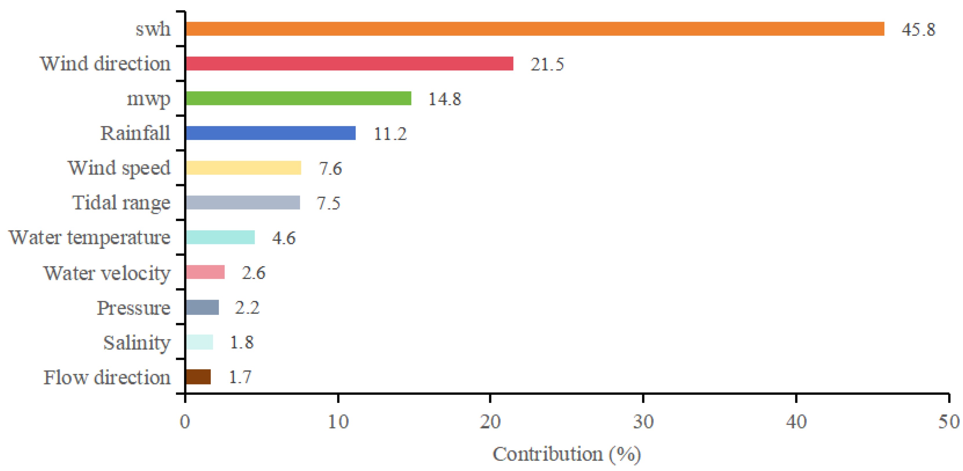
This paper collects data on as many as 12 characteristics related to SSC changes. The PCA algorithm can reduce the original feature data’s dimension and eliminate redundancy’s influence.

3.2.2. Long and Short-Term Memory Neural Network (LSTM)

The LSTM is a type of time-recurrent neural network that inherits most of the characteristics of the Recurrent Neural Network (RNN) model. Simultaneously, it solves the problem of gradient disappearance. Based on RNN, LSTM adds a “memory cell structure” for judging whether the information is valid or not, that is, a cell. We use the LSTM cell described in Figure 2 [6], which slightly simplifies the cell described by Graves et al. [22]. i, f, o, c, and g are vectors of input gates, acquisition gates, output gates, and cell activation and input modulation gates, respectively. Each cell includes an input gate, a forget gate, and an output gate. Each piece of data entering the LSTM network can be judged on whether it will be helpful for training [23]. Only useful information is retained, and information judged useless will be discarded through the forget gate [23]. This work proves effective for data exhibiting challenges related to long-term serial dependencies [24].

$$i_{\mathrm{t}}=\sigma (W_{xi}+W_{hi}{}_{t-1}+b_i)$$

(6)

$$i_{\mathrm{t}}=\sigma (W_{xi}+W_{hi}{}_{t-1}+b_i)$$

(7)

$$o_{\mathrm{t}}=\sigma (W_{xo}+W_{ho}{h}_{t-1}+b_o)$$

(8)

$$c_t=f_t\odot c_{t-1}+i_t\odot \tanh (W_{xc}{x}_t+W_{hc}{h}_{t-1}+b_c)$$

(9)

$$h_t=o_t\odot \tanh (c_t)$$

(10)

Wherein: ⊙ refers to the point multiplication of matrix by element; $b_{\gamma }$ is the deviation vector of each layer output; $\sigma (x)$ is the activation function; $W_{\alpha \beta }$ is the weight matrix of the corresponding layer; $c_t$ is used to update cell status; Input gate $i_t$ controls information flow into memory cell $c_t$; Output gate $o_t$ controls information in memory cell; $c_t$ at the current time can flow into the currently hidden $h_t$ [23].

3.2.3. Attention Mechanism

A model based on an attention mechanism [25] can quickly capture key regions in global information and focus on these regions to extract more helpful information. Adding an attention mechanism layer to LSTM enables the adaptive computation of attention weights based on the input sequence at each time step, facilitating better processing of long sequence inputs. At each time step, by computing the weight of each input, LSTM can better remember and utilize essential information in the feature data. The calculation formula for this is as follows:

$$u^t=\tanh (W_{{}^t}{h}_{{}^t})$$

(11)

$$\alpha \mathrm{t}=\frac{\exp (u_t{}^T{V}_t)}{{\displaystyle \sum _t\exp (u_t{}^T{V}_t)}}$$

(12)

$$\mathrm{s}={\displaystyle \sum _t{\alpha }_t{h}_t}$$

(13)

where W_t and V_t are parameters of the self-attention layer, h_t is the hidden state output at time step t, u_t is the attention score of the hidden state at time step t, α_t is the attention weight of the hidden state at time step t, and s is the final output of the self-attention layer [26].

3.2.4. Select Hyperparameters

Choosing appropriate hyperparameters for training LSTM is crucial. The differential evolution (DE) algorithm is an optimization algorithm that searches for optimization in the parameter space to determine the most suitable combination of hyperparameters [27]. The selected hyperparameters mainly include the learning rate, number of units in hidden layers, and batch size [16]. In order to improve the performance and computational efficiency, this paper uses the DE algorithm to determine the hyperparameters in the attention-based PCA-LSTM, PCA-LSTM, and LSTM models. The differential evolution algorithm is relatively robust when dealing with a small number of samples and high-dimensional problems because it does not require gradient calculations and conducts searches through differential operations and parameter variations. The differential evolution algorithm exhibits adaptability, allowing it to dynamically adjust based on the nature of the search space and adapt to the characteristics of different problems. This adaptability enables the differential evolution algorithm to perform well in various types of hyperparameter selection problems. The performance of LSTM networks is influenced by the choice of hyperparameters, and the differential evolution algorithm can search across the entire hyperparameter space, aiding in finding the optimal hyperparameter combination for performance.

3.2.5. Optimizing the PCA-LSTM Framework

(1)

Constructing a Multi-Source Dataset

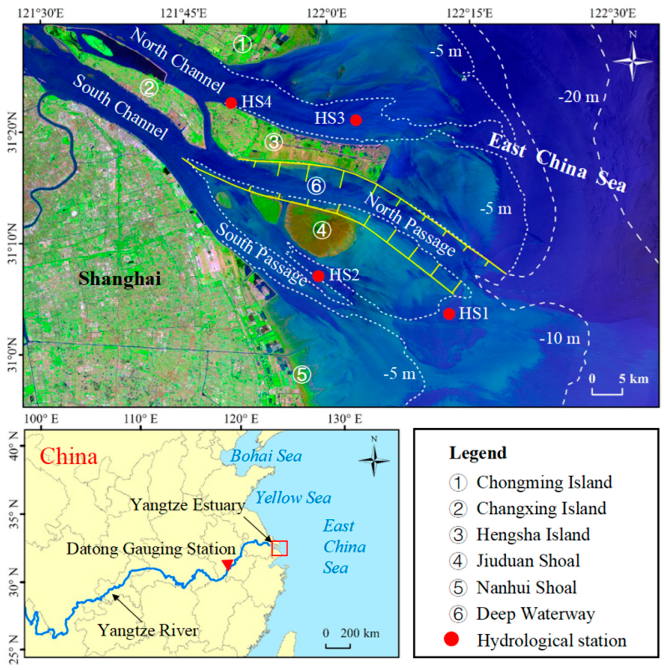
Merging data from multiple sources into a single dataset can be achieved through techniques such as time stamp alignment and matching of common keywords. Data from different sources may exhibit format differences, time disparities, or other inconsistencies. When merging data, these disparities can be addressed through techniques such as timestamp alignment and matching keywords, improving the consistency and quality of the data. This process of data cleaning and integration helps ensure that analyses are based on high-quality, consistent information. The high-precision meteorological data from ERA-5 provide critical information about meteorological conditions during typhoons. The observational data from the four hydrological stations at East China Normal University offer directly measured hydrological and water quality information, serving as an essential source for understanding the hydrological conditions in the estuarine region. Tidal range data from the Shanghai Maritime Safety Administration is of significant importance in comprehending the impact of tides and the transport of suspended sediments. By integrating data from these diverse sources, we gain a comprehensive understanding of the environmental conditions in the Yangtze River Estuary during typhoons, allowing for a thorough exploration of the variations in SSC and its relationship with meteorological and hydrological conditions.

(2)

Dealing with Non-Zero Missing Values

We addressed non-zero missing values in the multi-source dataset. Due to sensor malfunctions and data transmission issues during typhoons, missing values are inevitable, with the range of missing values within 5%. The linear interpolation method is employed to handle the missing values to avoid the impact of missing values on simulation SSC results.

Linear interpolation is a simple and efficient interpolation method. Despite the nonlinear trends in data, there exists local linearity between adjacent data points. In such cases, linear interpolation can sufficiently approximate the primary features of the data without introducing the additional complexity of higher-order interpolation.

Linear interpolation is calculated using the following formula:

$$Y=Y_{t-1}+\frac{(X_t^{}-X_{t-1})}{X_{t+1}-X_{t-1}}\times (Y_{t+1}-Y_{t-1})$$

(14)

Y_t is the estimate for a missing value, where Y_t−1 and Y_t+1 are adjacent known data points, and X_t is the position corresponding to the missing value. For each missing value, we first determine its temporal or spatial position X_t. Subsequently, we use the aforementioned linear interpolation formula to calculate the estimated value Y_t. This involves acquiring neighboring known data points, computing their rate of change, and using this information for interpolation. The calculated estimated value Y_t is then used to replace the missing value in the original dataset.

(3)

Normalization process

In order to accelerate the gradient descent process of the model, data normalization is performed. The formula for normalization is:

$$m=(x-x_{\min })/(x_{\max }-x_{\min })$$

(15)

In the formula, m represents the normalized value, x represents the original data, and $x_{\min }$ and $x_{\max }$ represent the minimum and maximum values of the original data sequence.

(4)

Data dimensionality reduction

Due to the raw data having a dimensionality of 12, using the raw data as input for the model directly would reduce the simulation effectiveness of the model and make it difficult to obtain satisfactory results within a reasonable training time. Therefore, reducing the dimensionality of the feature data is necessary to eliminate redundant information. PCA can transform multiple indicators into several comprehensive indicators (principal components) through orthogonal transformation, thereby reducing the interference of redundant data.

(5)

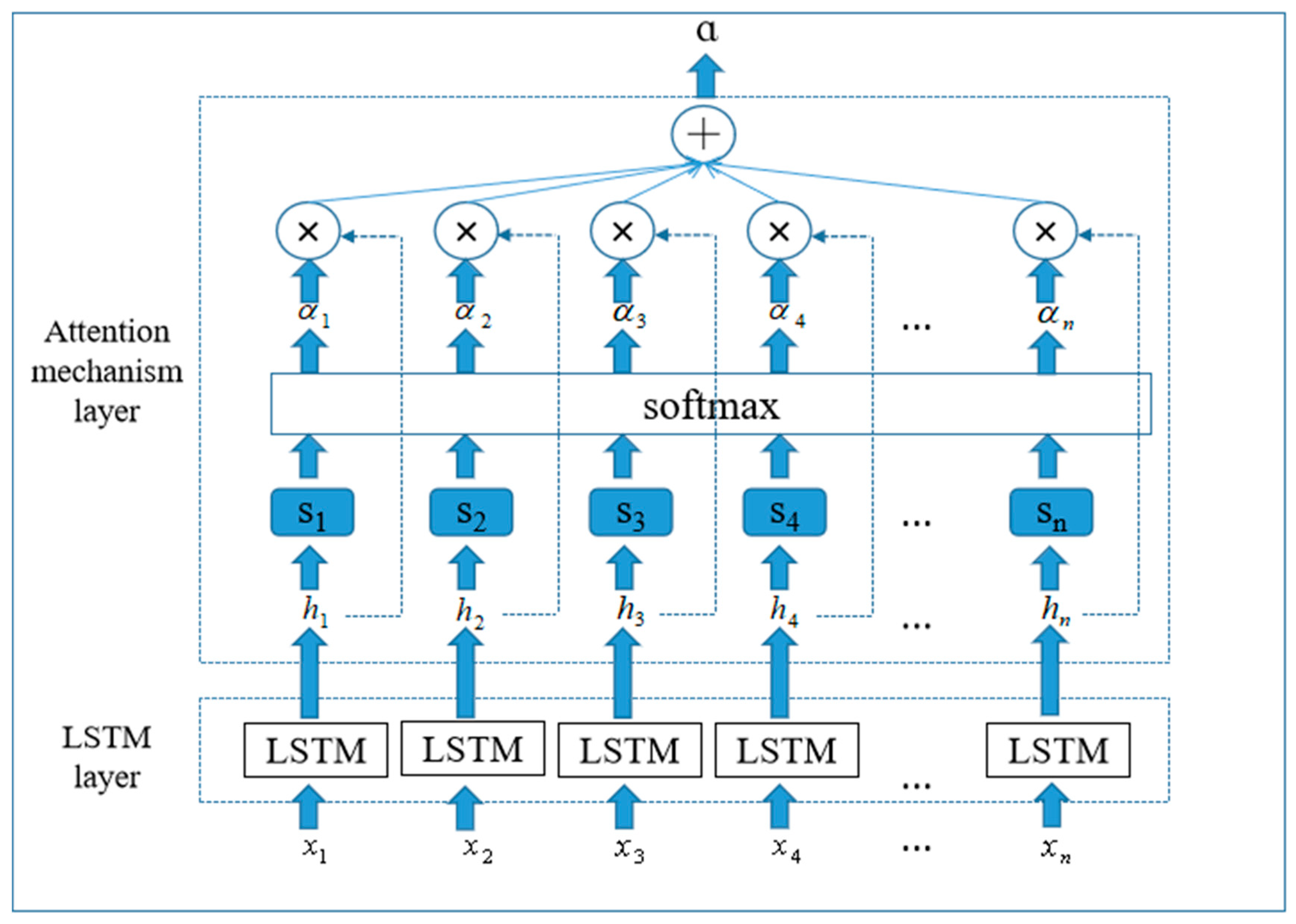
Add attention mechanism layer

Adding an attention mechanism layer in the LSTM network allows for the allocation of weights to different parts of the input sequence, improving the ability to focus on important information (Figure 3). The dimensionality-reduced data is fed into the LSTM layer, and the hidden state h_t is output for each time step. Unlike the unoptimized LSTM that uses the last hidden state to calculate the prediction, the attention-based LSTM inputs the hidden state for each time step into a self-attention layer. Through an attention scoring function, the self-attention layer calculates the attention distribution α, and then combines the h_t for each time step to calculate the final prediction, taking into account the h_t of the time step.

(6)

Parameter tuning and results output

In this paper, we use the DE algorithm to determine the hyperparameters of the LSTM network. The feature data reduced by the PCA method is used as the input variable for the model. The maximum training time is 100 with a training accuracy of 0.001, a learning rate of 0.01, a batch size of 5, 3 hidden layers with 9 hidden nodes, and the output variable is SSC. The model is trained using these settings to obtain the simulated SSC results.

3.2.6. Random Forest Model

This study employed a Random Forest model [28] to calculate the contribution rates of different influencing factors on SSC during typhoons. A higher contribution rate indicates a greater impact on SSC. The Random Forest algorithm calculates the contribution rate of each feature by measuring its splitting contribution when constructing decision trees. During the training process, each time a split is made, the algorithm records the splitting contributions of each feature and then averages these contributions across the entire forest. Feature importance is a relative measure, with larger values indicating a greater contribution of the feature to the model. Sorting by importance allows for the identification of variables that play a crucial role in the model.

3.2.7. Evaluating Indicator

Determination coefficient (R²), root mean square error (RMSE), mean square error (MSE), and mean absolute error (MAE) are used to evaluate the accuracy of the model. By evaluating these indicators for each research model, performance and accuracy are compared.

$${\mathrm{R}}^2={(\frac{{\displaystyle \sum XY}}{\sqrt{{\displaystyle \sum X^2{\displaystyle \sum Y^2}}}})}^2$$

(16)

$$\mathrm{RMSE}={[\frac{{\displaystyle \sum {(X-Y)}^2}}{N}]}^{0.5}$$

(17)

$$\mathrm{MSE}=\frac{{\displaystyle \sum {(X-Y)}^2}}{N}$$

(18)

$$\mathrm{MAE}=\frac{1}{\mathrm{n}}{\displaystyle \sum _{i=1}^{\mathrm{n}}|X-Y|}$$

(19)

X and Y are measured data and predicted values, respectively.

4. Results

4.1. Data Preprocessin

The data from four hydrological stations and meteorological data from the time of Typhoons Lekima, Hagupit, and In-Fa from 2019 to 2021 were used as the original data. Meteorological data from ECMWF, actual measured data from four East China Normal University hydrological stations, and tidal data from Shanghai Maritime Safety Administration were fused to construct a multi-source dataset. In data preprocessing, linear interpolation replaces non-zero missing values, normalization is performed, and then PCA is used for dimensionality reduction. The hourly data from Typhoon Lekima were used as the training set, the hourly data from Typhoon Hagupit were used as the validation set, and the hourly data from Typhoon In-Fa were used as the test set. Selecting hourly data from typhoon events and aligning it with the time of typhoon occurrences allows for the observation and capture of temporal changes in the characteristics of typhoon events. The PCA method used SPSS 25.0, and the DE algorithm and LSTM model were implemented using Python 3.7 and TensorFlow 2.0.

4.2. The Result of Data Dimensionality Reduction

The PCA was used to calculate each component and cumulative contribution rates. This helps to illustrate the contribution of each principal component to the total variance, aiding in identifying which principal components contain the most crucial information. The magnitude of the eigenvalues reflects the degree of variability in the data. Achieving a high cumulative contribution rate, principal components typically reflect the main features within the data. These principal components are crucial for identifying key information and potential trends in the data. By selecting eigenvectors corresponding to larger eigenvalues, the primary components of the data can be obtained. During the three typhoons, among the variables affecting the SSC of the HS1 hydrological station, the cumulative contribution value of the first seven principal components reached 92.68% (

Table 1. Calculation results of each principal component (HS1 & HS2).

		HS1			HS2
Principal Component	Eigenvalue	Percentage Variance	Cumulative	Eigenvalue	Percentage Variance	Cumulative
1	4.75	39.62	39.62	4.73	39.4	39.4
2	2.06	17.14	56.76	2.04	17.02	56.41
3	1.55	12.90	69.66	1.42	11.80	68.22
4	0.89	7.40	77.06	1.35	11.26	79.47
5	0.71	5.94	83.00	0.93	7.75	87.23
6	0.64	5.33	88.34	0.61	5.08	92.3
7	0.52	4.31	92.68	0.32	2.63	94.93
8	0.32	2.68	95.36	0.2	1.62	96.56
9	0.28	2.30	97.66	0.17	1.44	98.00
10	0.19	1.58	99.23	0.13	1.11	99.1
11	0.08	0.69	99.92	0.07	0.60	99.7
12	0.01	0.08	100	0.04	0.30	100

). Among the variables that affected the SSC of the HS2 hydrological station, the cumulative contribution value of the first six principal components reached 92.30% (Table 1). Among the variables that affected the SSC of the HS3 hydrological station, the cumulative contribution value of the first seven principal components reached 90.24% (

Table 2. Calculation results of each principal component (HS3 & HS4).

		HS3			HS4
Principal Component	Eigenvalue	Percentage Variance	Cumulative	Eigenvalue	Percentage Variance	Cumulative
1	4.23	35.23	35.23	4.21	35.04	35.04
2	2.00	16.69	51.92	2.54	21.17	56.22
3	1.34	11.19	63.12	1.86	15.48	71.70
4	1.10	9.18	72.30	0.98	8.17	79.87
5	1.00	7.92	80.22	0.72	6.00	85.87
6	0.72	6.02	86.24	0.50	4.18	90.05
7	0.48	4.01	90.24	0.44	3.70	93.75
8	0.45	3.77	94.02	0.31	2.57	96.32
9	0.38	3.12	97.14	0.19	1.55	97.87
10	0.27	2.21	99.35	0.15	1.21	99.07
11	0.07	0.57	99.91	0.08	0.70	99.77
12	0.01	0.09	100	0.03	0.23	100

). Among the variables affecting the SSC of the HS4 hydrological station, the cumulative contribution value of the first seven principal components reached 90.05% (Table 2). As the number of features increases, the correlation becomes more apparent, which means that not all feature quantities need to be calculated. Therefore, HS1 and HS3 select the first seven principal components and SSC as the input of the LSTM model, and HS2 and HS4 select the first six principal components and SSC as the input of the LSTM model. The similarities and differences of the principal component matrices of the four hydrological stations show that the PCA method can extract the data characteristics of different hydrological stations, and the principal components of different hydrological stations are significantly different (

Table 3. Principal component matrix (HS1).

	PC1	PC2	PC3	PC4	PC5	PC6	PC7
MWP	0.835	0.297	−0.376	−0.022	−0.035	−0.074	0.013
SWH	0.955	0.123	−0.159	−0.016	−0.071	−0.053	−0.027
Wind speed	0.935	0.115	−0.171	0.003	−0.086	−0.057	−0.014
Wind direction	−0.124	−0.449	0.773	0.051	0.003	0.057	−0.08
Water temperature	−0.587	0.658	−0.062	0.192	−0.13	0.046	−0.116
Pressure	−0.615	0.108	−0.376	0.174	0.303	−0.154	0.461
Salinity	0.332	−0.766	−0.164	−0.159	0.29	0.066	0.248
SSC	0.777	0.03	0.352	−0.215	0.021	−0.031	0.463
Water velocity	0.426	0.206	0.444	0.496	−0.268	0.104	−0.062
Tidal range	0.004	−0.524	−0.482	0.278	−0.275	0.551	0.096
Flow direction	0.089	0.615	0.16	−0.334	0.323	0.595	−0.282
Rainfall	0.477	0.032	0.071	0.615	0.55	0.017	0.103

,

Table 4. Principal component matrix (HS2).

	PC1	PC2	PC3	PC4	PC5	PC6
MWP	0.957	0.01	0.067	−0.057	0.025	−0.141
SWH	0.942	−0.036	0.029	0.002	0.044	−0.202
Wind speed	0.959	−0.006	0.093	0.021	0.025	−0.099
Wind direction	−0.865	−0.023	−0.177	0.334	0.124	0.004
Water temperature	−0.49	−0.24	0.753	0.084	0.15	−0.061
Pressure	0.771	−0.083	−0.242	0.463	0.01	−0.044
Salinity	−0.037	−0.525	−0.493	−0.546	−0.164	0.192
SSC	0.46	−0.251	0.166	0.51	−0.314	0.571
Water velocity	0.358	−0.233	−0.028	−0.222	0.81	0.315
Tidal range	0.028	0.838	−0.434	−0.093	−0.018	0.11
Flow direction	0.024	0.868	0.131	0.173	0.199	0.152
Rainfall	0.283	0.357	0.518	−0.606	−0.258	0.188

,

Table 5. Principal component matrix (HS3).

	PC1	PC2	PC3	PC4	PC5	PC6	PC7
MWP	−0.098	−0.098	−0.098	−0.098	−0.098	−0.098	−0.098
SWH	−0.169	−0.169	−0.169	−0.169	−0.169	−0.169	−0.169
Wind speed	−0.205	−0.205	−0.205	−0.205	−0.205	−0.205	−0.205
Wind direction	0.066	0.066	0.066	0.066	0.066	0.066	0.066
Water temperature	−0.115	−0.115	−0.115	−0.115	−0.115	−0.115	−0.115
Pressure	−0.122	−0.122	−0.122	−0.122	−0.122	−0.122	−0.122
Salinity	0.006	0.006	0.006	0.006	0.006	0.006	0.006
SSC	0.09	0.09	0.09	0.09	0.09	0.09	0.09
Water velocity	0.41	0.41	0.41	0.41	0.41	0.41	0.41
Tidal range	−0.099	−0.099	−0.099	−0.099	−0.099	−0.099	−0.099
Flow direction	0.297	0.297	0.297	0.297	0.297	0.297	0.297
Rainfall	0.307	0.307	0.307	0.307	0.307	0.307	0.307

and

Table 6. Principal component matrix (HS4).

	PC1	PC2	PC3	PC4	PC5	PC6
MWP	0.928	0.248	0.017	0.026	−0.074	−0.112
SWH	0.955	0.106	−0.08	0.002	−0.103	−0.016
Wind speed	0.915	−0.059	−0.09	−0.096	−0.171	0.189
Wind direction	0.79	0.348	0.339	−0.135	−0.102	0.083
Water temperature	−0.33	0.361	0.712	−0.038	−0.039	−0.251
Pressure	−0.203	−0.247	0.78	0.262	0.04	0.373
Salinity	0.066	0.667	0.151	0.558	0.032	−0.297
SSC	0.754	−0.389	−0.056	0.277	0.27	−0.118
Water velocity	0.377	−0.659	0.373	0.384	0.089	0.041
Tidal range	−0.163	0.751	−0.098	0.295	−0.363	0.29
Flow direction	0.039	0.631	−0.338	0.125	0.609	0.237
Rainfall	0.279	0.399	0.568	−0.495	0.275	0.016

).

4.3. Parameter Setting

The setting of hyperparameters is primarily achieved through the DE algorithm, which calculates and selects the optimal hyperparameters. In this study, the best hyperparameter set is chosen by comparing the optimal simulation results of the SSC corresponding to models with different hyperparameter values generated during training. Different parameter configurations can significantly impact the performance of the model, as altering hyperparameters such as population size, number of iterations, scaling factor, and crossover factor can affect the model’s search space and generalization ability. The hyperparameters are set at: population size NP = 10, iteration number G = 20, scaling factor F = 0.6, and crossover factor CR = 0.8 [16]. For LSTM networks, the learning rate is specified in the range [0, 1], the number of hidden layer units is specified in the range [1, 100], and the batch size is specified in the range [1, 100]. The hyperparameter settings of LSTM are shown in

Table 7. Parameter settings.

Model	Parameters	Value	Reason
Attention-based PCA-LSTM PCA-LSTM LSTM	Learning rate	0.0038	Obtained by DE
	Hidden unit	34	Obtained by DE
	Batch size	14	Obtained by DE
	Epochs of training	500	Converged

. For LSTM networks, the learning rate is specified in the range [0, 1], the number of hidden layer units is in the range [1, 100], and the range of batches varies. Each model was run independently five times, and finally, their average value was taken as the training result. The parameters were made with the same settings to ensure that the parameters did not affect the simulation results of the attention-based PCA-LSTM, PCA-LSTM, and LSTM models.

4.4. Simulation Results

4.4.1. Simulation Results of Attention-Based PCA-LSTM

As shown in Figure 4, the simulation results of attention-based PCA-LSTM exhibit a good fitting performance with the observed SSC data for the four hydrological stations in the Yangtze River Estuary, regardless of the peaks or the lows. There is a high level of consistency between the actual SSC and the simulation results. Moreover, the fitting R² coefficients of the SSC simulation results for the HS1, HS2, HS3, and HS4 hydrological stations are 0.876, 0.875, 0.866, and 0.856, respectively, and all R² are higher than 0.85. This indicates that the simulation results based on the attention-based PCA-LSTM framework have an excellent fitting effect with the actual SSC. The relevant results of each hydrological station are relatively stable with little difference. In addition, the superiority of the simulation results is evident in their excellent matching with peaks and troughs. This means that the model, while simulating SSC, can accurately capture the observed peaks and troughs at hydrological stations. It provides a reliable simulation of crucial events in actual hydrology. The robust performance in these aspects further enhances the credibility of attention-based PCA-LSTM in simulating SSC.

4.4.2. Simulation Results of PCA-LSTM

In the results of the PCA-LSTM model, as shown in Figure 5, the fitting R² coefficients of the simulated SSC of the hydrological stations HS1, HS2, HS3, and HS4 are 0.801, 0.814, 0.792, and 0.778, respectively. The fitting R² coefficients of HS3 and HS4 are below 0.8, indicating that the PCA-LSTM model performs better in simulating the SSC of HS1 and HS2. At the same time, the simulation of SSC for HS3 and HS4 did not achieve the expected results. Overall, there is poor consistency between the actual SSC and the simulation results.

4.4.3. Simulation Results of the Traditional LSTM Model

The results are shown in Figure 6. The traditional LSTM model almost overestimates the peak values of SSC at the four hydrological stations. There is also a significant overestimation of the minimum values of SSC at the four hydrological stations. The agreement between the actual SSC and the simulation results is poor. Furthermore, in the LSTM model results, the R² of SSC simulation results for hydrological stations HS1, HS2, HS3, and HS4 are 0.538, 0.557, 0.546, and 0.57, respectively. It can be seen that the simulation results of the traditional LSTM model do not fit well with the actual SSC.

5. Discussion

5.1. Improvement of PCA-LSTM Simulation Results with the Introduction of the Attention Mechanism

This study explores the influence of integrating an attention mechanism into the PCA-LSTM framework on the simulated SSC results from the Yangtze River Estuary during Typhoon In-Fa. Furthermore, a comparison between the attention-based PCA-LSTM framework and the original PCA-LSTM framework was conducted. The results indicate that the attention-based PCA-LSTM outperforms the original PCA-LSTM regarding simulation accuracy. The attention mechanism enables the LSTM to focus more on the essential features that affect the SSC, resulting in lower RMSE of the simulation results. The attention-based PCA-LSTM produces lower RMSE values for the simulated SSC at the four hydrological stations in the Yangtze River Estuary, with values of 0.188, 0.209, 0.149, and 0.172, respectively, which are lower than those obtained with the original PCA-LSTM (

Table 8. Error statistics (Attention-based PCA-LSTM).

Hydrological Station	RMSE	MSE	MAE
HS1	0.188	0.035	0.114
HS2	0.209	0.044	0.139
HS3	0.149	0.022	0.101
HS4	0.172	0.029	0.122

and

Table 9. Error statistics (PCA-LSTM).

Hydrological Station	RMSE	MSE	MAE
HS1	0.218	0.048	0.136
HS2	0.232	0.054	0.151
HS3	0.215	0.046	0.138
HS4	0.221	0.049	0.148

). Specifically, the attention mechanism allows the LSTM model to assign weights to different input features at each time step, emphasizing the most relevant features to the SSC at the current time step. The attention mechanism possesses adaptability, allowing it to adjust weights based on the importance of input data. When dealing with heterogeneous data from different sources, the attention mechanism can effectively modify its focus, ensuring a more targeted capture of crucial information related to SSC during typhoon events. Adding an attention mechanism layer to the PCA-LSTM allows the model to effectively capture the nonlinear relationship between the essential features and the SSC under typhoon weather conditions, resulting in more accurate simulations. The attention mechanism adaptively adjusts the weights of the input features based on their relevance to the current time step, allowing the model to effectively capture the temporal variations of the feature data and improve the model’s generalization capability, resulting in more accurate simulations.

The changes in meteorological and hydrological factors exhibit different characteristics during different time intervals in typhoons. When simulating SSC during typhoons, certain time steps may be more critical for the variation of SSC. When dealing with the uncertainty of meteorological and hydrological factors, the attention mechanism enables the model to adaptively focus on crucial moments of SSC changes and key features, thereby selectively enhancing its perception of SSC changes during different periods in typhoons. PCA typically assumes that the principal components are orthogonal, while in practical situations, there may be correlations among different meteorological and hydrological features. Attention mechanisms can assist the model in better balancing the importance of features when dealing with highly correlated features, enhancing sensitivity to feature correlations in the input data. In the PCA-LSTM framework, principal component analysis (PCA) is introduced for dimensionality reduction, but certain principal components may contribute more to SSC prediction. Through attention mechanisms, the model can automatically learn the weights of each principal component, adjusting their impact on predictions to better align with real-world scenarios.

5.2. Effect of Input Variables on Model

The dynamical processes of typhoons can lead to the resuspension of seafloor sediments, with a significant increase in the volumetric concentration of suspended material and the increase in land-sourced material due to the high-intensity rainfall accompanying typhoons [29]. Previous studies have found that many factors caused by typhoons, among others, can significantly influence the changes in SSC [30]. Therefore, the PCA method can calculate the input variables significantly correlated with the SSC changes during Typhoon In-Fa. This study clearly shows that the appropriate input variables enable the model to effectively simulate the changes in SSC during Typhoon In-Fa. Compared with the traditional LSTM model, the magnitude of the PCA-LSTM framework is closer to the observed values for low, medium, and high SSC simulations. The PCA-LSTM framework is better than the traditional LSTM model for SSC simulations during Typhoon In-Fa. In addition, the R² of the four hydrological stations at the Yangtze Estuary reached 0.801, 0.814, 0.792, and 0.778 using the PCA-LSTM to simulate the SSC of each. Compared with the traditional LSTM model, estimates improved by 26.3%, 25.7%, 24.6%, and 20.0%, respectively. Since PCA reduces the dimensionality of the training data and selects the main input variables of the LSTM model during typhoons, it improves the output accuracy of the model results. The traditional LSTM model is unable to effectively calculate the primary components influencing the variation of SSC in the data, and the high dimensionality of input data results in lower accuracy for some outcomes. This limitation stems from the inherent constraints of the LSTM model in handling high-dimensional data. The PCA-LSTM framework can solve the above problems. Comparing the two models shows that the choice of variable inputs is indispensable for deep learning methods. This shows that PCA can orthogonally transform multiple indicators into multiple composite indicators (principal components) with less missing data, avoid redundant interference, and use the feature data after eliminating redundancy in the input of the LSTM model to improve the accuracy of SSC simulation.

To validate the contributions of different variables to the nonlinear changes in SSC during typhoons, this study employed a Random Forest model to rank the importance of the 11 variables. The top four variables in terms of contribution rates were SWH, Wind direction, MWP, and Rainfall, with contribution rates of 45.8%, 21.55%, 14.8%, and 11.25%, respectively (Figure 7). Their combined contribution reached 93.35%, significantly surpassing other factors. These results indicate that SWH, Wind direction, MWP, and Rainfall play pivotal roles in simulating the nonlinear changes in SSC during typhoons. Specifically, SWH reflects the energy of ocean waves, Wind direction indicates the direction of wind influencing the transport of suspended sediments, MWP may be related to the periodic changes in ocean waves, and Rainfall could potentially affect SSC variations through runoff triggered by precipitation. The high contribution rates of these factors underscore their importance in influencing the performance and accuracy of the model.

5.3. Validity of the Attention-Based PCA-LSTM Framework

RMSE [31], MSE, and MAE have been widely used as evaluation metrics to evaluate models’ effectiveness in numerous deep learning studies [32,33,34,35,36]. In this study, in order to verify the effectiveness of the attention-based PCA-LSTM framework in simulating the SSC during Typhoon In-Fa, we used different evaluation indicators such as RMSE, MSE, and MAE for evaluation. We compare it with the PCA-LSTM framework without introducing the attention mechanism and the traditional LSTM model. The more significant the difference between RMSE and MAE, the more significant the variance of individual errors in the sample [37]. If RMSE is equal to MAE, then all errors are equally significant. Table 9 shows that the attention-based PCA-LSTM framework has the slightest difference between RMSE and MAE, which are 0.074, 0.070, 0.048, and 0.050, respectively. In contrast, the difference in RMSE and MAE between PCA-LSTM and LSTM is more significant than that of attention-based PCA-LSTM, indicating that the attention-based PCA-LSTM has better stability than the PCA-LSTM and traditional LSTM models (Table 9 and

Table 10. Error statistics (LSTM).

Hydrological Station	RMSE	MSE	MAE
HS1	0.572	0.327	0.417
HS2	0.543	0.295	0.325
HS3	0.330	0.109	0.161
HS4	0.435	0.189	0.245

). Figure 8 shows the simulation error ranges of [−0.848, 0.617], [−0.703, 0.683], [−0.665, 0.533], and [−0.562, 0.661] for the four hydrological stations using the attention-based PCA-LSTM. Figure 9 shows the simulation error ranges of [−0.614, 0.616], [−0.769, 0.686], [−0.668, 0.740], and [−0.735, 0.561] for the four hydrological stations using the PCA-LSTM. Figure 10 shows the simulation error ranges of [−1.329, 2.103], [−1.869, 1.966], [−1.518, 1.864], and [−1.355,1.635] for the four hydrological stations using the traditional LSTM model. It can be seen that the attention-based PCA-LSTM has a smaller error interval on the whole. The RMSE, MSE, and MAE of the attention-based PCA-LSTM during Typhoon In-Fa were better than those of the PCA-LSTM and traditional LSTM models. The overall error was slightly lower than that of the PCA-LSTM and significantly lower than that of the traditional LSTM model. This indicates that the simulation results of the attention-based PCA-LSTM work better within an acceptable error range. Therefore, the attention-based PCA-LSTM has better stability in the simulation results of SSC during Typhoon In-Fa, and the error accuracy of the attention-based PCA-LSTM is better than that for the PCA-LSTM and traditional LSTM model in the simulation of SSC, which proves the effectiveness of the attention-based PCA-LSTM framework.

6. Conclusions

To evaluate the simulation performance of the attention-based PCA-LSTM framework on the SSC during Typhoon In-Fa, the R² metric was used to assess the simulation accuracy, while the RMSE, MSE, and MAE metrics were employed to quantify the precision of the model error. The following key conclusions can be drawn:

(1)

The attention-based PCA-LSTM framework showed significant optimization in all evaluation metrics. Compared with the original PCA-LSTM framework and traditional LSTM models, the attention-based PCA-LSTM framework demonstrated improved performance and generalization ability on the same dataset, with higher accuracy and a lower overall error rate.

(2)

The input variables have a significant impact on improving the model’s accuracy. The PCA-LSTM framework with feature data input that has been dimension-reduced achieved higher accuracy in the SSC simulation than traditional LSTM models. The PCA method effectively eliminates the interference of redundant data on the model, thus improving the accuracy of simulating SSC.

(3)

The simulation performance of the attention-based PCA-LSTM framework is superior to that of the original PCA-LSTM framework and traditional LSTM models. Although deep neural networks have demonstrated exemplary performance in hydrology and we obtained satisfactory results, the black-box nature of deep neural networks remains a challenging problem to overcome.

The geographical environments and climatic conditions differed among the various estuarine systems, leading to distinct meteorological and hydrological conditions. Due to certain constraints, this study could only obtain SSC data from the Yangtze Estuary. In future research, we plan to apply the attention-based PCA-LSTM model to different estuarine systems, incorporating hydrological, meteorological, and tidal data from diverse estuarine regions into the model for cross-regional validation. This approach aims to enhance the model’s applicability across varied geographical environments and meteorological conditions. Challenges faced by this study and subsequent research include balancing data quality, model complexity, and computational costs, as well as understanding the long-term impacts of extreme weather events. Our future research will focus on addressing these challenges to improve the practicality of the model. Furthermore, given the substantial contribution of swh to SSC, water depth is also recognized as a crucial parameter, especially in estuarine research. However, due to limitations in the instrumentation of hydrological stations, water depth data were not acquired. In subsequent research, we plan to incorporate water depth data into the multi-source dataset and use it as an input for the model.

References

1. Schoellhamer, D.H.; Mumley, T.E.; Leatherbarrow, J.E. Suspended sediment and sediment-associated contaminants in San Francisco Bay. Environ. Res. 2007, 105, 119–131. [Google Scholar] [CrossRef] [PubMed]
2. Wang, H.; Yang, S.; Yang, H. A study of the surficial suspended sediment concentration in response to typhoons in the Yangtze Estuary. J. East China Norm. Univ. (Nat. Sci.) 2019, 2019, 195. [Google Scholar]
3. Tang, R.; Shen, F.; Ge, J.; Yang, S.; Gao, W. Investigating typhoon impact on SSC through hourly satellite and real-time field observations: A case study of the Yangtze Estuary. Cont. Shelf Res. 2021, 224, 104475. [Google Scholar] [CrossRef]
4. Dang, T.D.; Cochrane, T.A.; Arias, M.E. Quantifying suspended sediment dynamics in mega deltas using remote sensing data: A case study of the Mekong floodplains. Int. J. Appl. Earth Obs. Geoinf. 2018, 68, 105–115. [Google Scholar] [CrossRef]
5. Nourani, V.; Behfar, N. Multi-station runoff-sediment modeling using seasonal LSTM models. J. Hydrol. 2021, 601, 126672. [Google Scholar] [CrossRef]
6. Kaveh, K.; Kaveh, H.; Bui, M.D.; Rutschmann, P. Long short-term memory for predicting daily suspended sediment concentration. Eng. Comput. 2021, 37, 2013–2027. [Google Scholar] [CrossRef]
7. Huang, C.C.; Chang, M.J.; Lin, G.F.; Wu, M.C.; Wang, P.H. Real-time forecasting of suspended sediment concentrations reservoirs by the optimal integration of multiple machine learning techniques. J. Hydrol. Reg. Stud. 2021, 34, 100804. [Google Scholar] [CrossRef]
8. Le, X.H.; Ho, H.V.; Lee, G.; Jung, S. Application of long short-term memory (LSTM) neural network for flood forecasting. Water 2019, 11, 1387. [Google Scholar] [CrossRef]
9. Gao, S.; Huang, Y.; Zhang, S.; Han, J.; Wang, G.; Zhang, M.; Lin, Q. Short-term runoff prediction with GRU and LSTM networks without requiring time step optimization during sample generation. J. Hydrol. 2020, 589, 125188. [Google Scholar] [CrossRef]
10. Zhang, Y.; Zhang, C.; Zhao, Y.; Gao, S. Wind speed prediction with RBF neural network based on PCA and ICA. J. Electr. Eng. 2018, 69, 148–155. [Google Scholar] [CrossRef]
11. Yang, D.; Chen, K.; Yang, M.; Zhao, X. Urban rail transit passenger flow forecast based on LSTM with enhanced long-term features. IET Intell. Transp. Syst. 2019, 13, 1475–1482. [Google Scholar] [CrossRef]
12. Zhang, J.; Zhu, Y.; Zhang, X.; Ye, M.; Yang, J. Developing a Long Short-Term Memory (LSTM) based model for predicting water table depth in agricultural areas. J. Hydrol. 2018, 561, 918–929. [Google Scholar] [CrossRef]
13. Zhang, Y.; Chen, B.; Pan, G.; Zhao, Y. A novel hybrid model based on VMD-WT and PCA-BP-RBF neural network for short-term wind speed forecasting. Energy Convers. Manag. 2019, 195, 180–197. [Google Scholar] [CrossRef]
14. Sarker, I.H.; Abushark, Y.B.; Khan, A.I. Contextpca: Predicting context-aware smartphone apps usage based on machine learning techniques. Symmetry 2020, 12, 499. [Google Scholar] [CrossRef]
15. Yang, K.; Yuan, J.L.; Xiong, T.; Wang, B.; Fan, S.D. A novel principal component analysis integrating long short-term memory network and its application in productivity prediction of cutter suction dredgers. Appl. Sci. 2021, 11, 8159. [Google Scholar] [CrossRef]
16. Geng, D.; Zhang, H.; Wu, H. Short-term wind speed prediction based on principal component analysis and LSTM. Appl. Sci. 2020, 10, 4416. [Google Scholar] [CrossRef]
17. Huang, M.H.; Zhang, Q.L.; Guan, J.Y. A cellular automata model for population expansion of spartina alterniflora at jiuduansha shoals, shanghai, china. Estuar. Coast. Shelf Sci. 2008, 77, 47–55. [Google Scholar] [CrossRef]
18. Ma, J.; Yuan, Y. Dimension reduction of image deep feature using PCA. J. Vis. Commun. Image Represent. 2019, 63, 102578. [Google Scholar] [CrossRef]
19. Liu, B.; Yang, R. A novel method based on PCA and LS-SVM for power load forecasting. In Proceedings of the 2008 Third International Conference on Electric Utility Deregulation and Restructuring and Power Technologies, Nanjing, China, 6–9 April 2008; IEEE: Piscataway Township, NJ, USA, 2008. [Google Scholar]
20. Chi, L.; Huang, Y.; Liu, C.; Wang, Y.; Liang, Z. Research on Evaluation Method of Renewable Energy Accommodation Capability Based on LSTM. In Proceedings of the 2018 2nd IEEE Conference on Energy Internet and Energy System Integration (EI2), Beijing, China, 20–22 October 2018; IEEE: Piscataway Township, NJ, USA, 2018. [Google Scholar]
21. Zheng, Y.; Wu, X.L.; Zhao, D.; Xu, Y.W.; Li, X. Data-driven fault diagnosis method for the safe and stable operation of solid oxide fuel cells system. J. Power Sources 2021, 490, 229561. [Google Scholar] [CrossRef]
22. Graves, A.; Jaitly, N. Towards end-to-end speech recognition with recurrent neural networks. In International Conference on Machine Learning; PMLR: London, UK, 2014; pp. 1764–1772. [Google Scholar]
23. Yu, Z.; Yang, K.; Luo, Y.; Shang, C. Spatial-temporal process simulation and prediction of chlorophyll-a concentration in dianchi lake based on wavelet analysis and long-short term memory network. J. Hydrol. 2020, 582, 124488. [Google Scholar] [CrossRef]
24. Memory, L.S.T. Long Short-Term. Long short-term memory. Neural Comput. 2010, 9, 1735–1780. [Google Scholar]
25. Laghrissi, F.E.; Douzi, S.; Douzi, K.; Hssina, B. Ids-attention: An efficient algorithm for intrusion detection systems using attention mechanism. J. Big Data 2021, 8, 149. [Google Scholar] [CrossRef]
26. Ma, T.; Xiang, G.; Shi, Y.; Liu, Y. Horizontal in situ stresses prediction using a cnn-bilstm-attention hybrid neural network. Geomech. Geophys. Geo-Energy Geo-Resour. 2022, 8, 152. [Google Scholar] [CrossRef]
27. Wang, L.; Zeng, Y.; Chen, T. Back propagation neural network with adaptive differential evolution algorithm for time series forecasting. Expert Syst. Appl. 2015, 42, 855–863. [Google Scholar] [CrossRef]
28. Rigatti, S.J. Random forest. J. Insur. Med. 2017, 47, 31–39. [Google Scholar] [CrossRef]
29. Li, Y.; Li, D.; Fang, J.; Yin, X.; Li, H.; Hu, W.; Chen, J. Impact of Typhoon Morakot on suspended matter size distributions on the East China Sea inner shelf. Cont. Shelf Res. 2015, 101, 47–58. [Google Scholar] [CrossRef]
30. Zhang, Z.; Song, Z.; Lu, F. A numerical study on storm surge and sediment Resuspending in Modaomen Estuary during Typhoon Hagupit. In International Conference on Offshore Mechanics and Arctic Engineering; American Society of Mechanical Engineers: New York, NY, USA, 2013. [Google Scholar]
31. Sun, W.; Zhou, S.; Yang, J.; Gao, X.; Ji, J.; Dong, C. Artificial Intelligence Forecasting of Marine Heatwaves in the South China Sea Using a Combined U-Net and ConvLSTM System. Remote Sens. 2023, 15, 4068. [Google Scholar] [CrossRef]
32. Mehri, Y.; Nasrabadi, M.; Omid, M.H. Prediction of suspended sediment distributions using data mining algorithms. Ain Shams Eng. J. 2021, 12, 3439–3450. [Google Scholar] [CrossRef]
33. Shamaei, E.; Kaedi, M. Suspended sediment concentration estimation by stacking the genetic programming and neuro-fuzzy predictions. Appl. Soft Comput. 2016, 45, 187–196. [Google Scholar] [CrossRef]
34. Li, S.; Xie, Q.; Yang, J. Daily suspended sediment forecast by an integrated dynamic neural network. J. Hydrol. 2022, 604, 127258. [Google Scholar] [CrossRef]
35. Zhang, X.; Yang, Y. Suspended sediment concentration forecast based on CEEMDAN-GRU model. Water Supply 2020, 20, 1787–1798. [Google Scholar] [CrossRef]
36. Rezaei, K.; Pradhan, B.; Vadiati, M.; Nadiri, A.A. Suspended sediment load prediction using artificial intelligence techniques: Comparison between four state-of-the-art artificial neural network techniques. Arab. J. Geosci. 2021, 14, 215. [Google Scholar] [CrossRef]
37. Chai, T.; Draxler, R.R. Root mean square error (RMSE) or mean absolute error (MAE)?–Arguments against avoiding RMSE in the literature. Geosci. Model Dev. 2014, 7, 1247–1250. [Google Scholar] [CrossRef]
Figure 1. Map of the study area.
Water 16 00146 g001
Figure 2. LSTM cell structure. (i, f, o, c, and g are vectors of input gates, acquisition gates, output gates, and cell activation and input modulation gates, respectively).
Water 16 00146 g002
Figure 3. Attention mechanism layer structure.
Water 16 00146 g003
Figure 4. Attention-based PCA-LSTM simulation results and actual SSC.
Water 16 00146 g004
Figure 5. PCA-LSTM simulation results and actual SSC.
Water 16 00146 g005
Figure 6. LSTM simulation results and actual SSC.
Water 16 00146 g006
Figure 7. Contribution rates of different variables to SSC.
Water 16 00146 g007
Figure 8. Test Set Prediction Error (Attention-based PCA-LSTM).
Water 16 00146 g008
Figure 9. Test Set Prediction Error (PCA-LSTM).
Water 16 00146 g009
Figure 10. Test Set Simulation Error (LSTM).
Water 16 00146 g010