Article

Forecasting Urban Peak Water Demand Based on Climate Indices and Demographic Trends

by
Anika Stelzl
* and
Daniela Fuchs-Hanusch
Institute of Urban Water Management and Landscape Water Engineering, Graz University of Technology, Stremayrgasse 10/I, 8010 Graz, Austria
*
Author to whom correspondence should be addressed.
Water 2024, 16(1), 127; https://doi.org/10.3390/w16010127
Submission received: 30 November 2023 / Revised: 21 December 2023 / Accepted: 25 December 2023 / Published: 29 December 2023

Abstract

:
Austria’s water utilities are facing new challenges due to advancing climate change. In recent years, changes in water demand have been observed. Water demand forecast models are required to assess these changes and react to them in a sustainable way. In this study, an existing modeling approach was extended with new climate indices. The multiple linear regression model was applied to different study sites. The model was trained with a training dataset and validated with a test dataset. The performance of the model was assessed using common parameters, such as the mean absolute percentage error. In a further step, the modeling approach was applied to climate projections to estimate the change in water demand for three different representative concentration pathways (RCPs). The change in water demand due to population growth was then considered and combined with the change due to climate change. RCP2.6 shows an average 14% increase in water demand for the period 2051–2070, with climate change (average increase of 0.7%) playing a negligible role. For RCP4.5, an increase of 16% is predicted, while the highest increase of 19% is observed in RCP8.5. Population growth is responsible for most of the increase.

1. Introduction

Several factors, such as population growth, urbanization, wealth, and climate change, are influencing water demand in urban areas. [1,2,3,4]. The relationship between these influencing parameters and the change in water demand has been investigated in several studies. For example, Dimkić [1] determined the influence of temperature on water consumption for two large cities in Serbia. The research showed that temperature plays a significant role in influencing water demand. In a further study [5], the effects of climate variables on household water demand in three geographically distributed cities in Ethiopia were investigated. The authors discovered a significant correlation between the examined climate parameters and water consumption. A study in Austria [6] showed a correlation between water demand, temperature, and dry periods. It was found that the daily water demand also increases as the temperatures increase. In addition, the results showed that peak water demand occurs with rising temperatures.
Based on these findings, appropriate forecast models are required for long-term predictions so that utilities can react to these changes in a sustainable manner. Multiple studies on water demand forecast models can be found in the literature [7]. However, the majority of the studies focus on optimizing system operation and not on long-term forecasts [8]. Different modeling approaches can be used for water demand forecasts, for example, multiple linear regression (MLR) [9,10], artificial neural networks (ANN) [11,12], or support vector regression (SVR) [13].
Bakker et al. [14] found that weather data can improve water demand forecasting. Donevska and Panov [15] employed multi-regression models to demonstrate how climate change affects water demand. In this regard, they analyzed the relationship between water supply data, precipitation, and temperature.
A study [16] was carried out to demonstrate the impact of climate change on water demand in Naples. The goal was to establish a connection between water demand and weather using coupled general circulation models. Atmospheric and oceanic processes were simulated using the models. Furthermore, random forest models (RF) were used to show the relationship between water demand and weather. The research showed that water demand may increase by 9–10% when maximum temperatures occur. Additionally, it was discovered that social characteristics (employment and level of education) have an influence on water demand.
Ashoori, Dzombak, and Small [3] used multiple linear regression models to investigate the influence of various factors, such as climate, demographics, and water price, on water demand. It was found that price and population had the greatest influence. Furthermore, temperature and precipitation turned out to be very significant. A daily demand model based on the stepwise regression approach was derived for the city of Toronto [8]. It was found that when the temperature increases by 1 degree, the peak water demand in summer will increase by 1.8% and the average water demand by 2%.
In a study in Montreal [17], a clustering analysis was performed that categorized water consumption into basic and seasonal consumption. The authors found that baseline water consumption is influenced by weekends but is independent of climate change, and seasonal water demand is dependent on the air temperature and total precipitation. Furthermore, in this study, linear Bayesian regression was applied, and climate projections were included for prediction. The results show a trend toward increasing seasonal water consumption.
Vonk et al. [13] used an SVR model to predict daily water demand for the year 2050 based on meteorological parameters and variations in vacation absence/presence (tourism). This information was then coupled with an extreme value model. The study considered various climate change scenarios and they also considered vacation scenarios. The authors found that the peak water demand increases by 6.5% and the average water demand only increases by 0.8% by 2050.
In a previous study [10] by the authors, a general MLR model was derived that considers climate indices. In this study, the results of the MLR modeling approach were compared with the results of other modeling approaches, which were SVR, RF, and ANN. We found that the general MLR modeling approach provided equivalent results to the other modeling approaches. Climate projections based on the representative concentration pathway (RCP) were considered. The water demand for the RCP8.5 was predicted, and we found that the peak water demand will increase in Austria during the summer months. In this study, other RCPs and demographic trends were not considered.
Water demand forecast models for long-term forecasts that consider both changes due to climate change and socio-demographic developments are needed. They are the basis for robust and sustainable decisions to maintain future water supply.
Therefore, in this study, the modeling approach from the previous study [10] was expanded. The aim is to obtain a model that can be applied to other inflow measurements without great effort. The initial studies have shown that the peak water demand due to drought conditions only decreases after larger amounts or durations of precipitation. Based on these findings, new climate indices were derived and used for the present study. These are e.g., dry hot days or maximum air temperature. Additionally, demographic change was considered. The aim of this work is to estimate future peak water demand based on climate change and demographic development. In the first step, the relationship between water demand and climate indices is determined. A suitable regression model is then derived, which can be applied to climate projections. Three available climate change scenarios RCP2.6, RCP4.5, and RCP8.5 are used for the water demand prediction to show how water demand can develop based on the different scenarios. In a further step, population change is included and a possible total change in future water demand is determined.
This work has the following structure. In the materials section, we describe the study sites and the used data. Next, we provide an overview of the workflow and modeling approach in the method section. The performance evaluation of the regression model and the discussion of the water demand prediction results are presented in the results section. In the final section, we present our conclusions.

2. Materials

2.1. Study Site

Four study sites in Austria were considered, which have a warm temperate climate and fully humid and warm summers.
The Austrian water utilities maintain records of their daily water demand, which is depicted through the daily inflow into the system or specific zones. In this study, we assume that water losses are small and remain consistent throughout the measured period. There is hardly any tourist activity in any of the zones and this aspect is, therefore, neglected.
The inflow into the zone was measured for all zones and is available at a daily resolution (m3/d). Multi-year water demand records were available for all the zones. For Zone 1 and Zone 3, 10 years were available in each case and 8 years were available for zones 2 and 4. The water demand records were provided to us by the responsible water utilities.
Zone 1 and Zone 2 are large districts with a large proportion of single-family households and multi-family households and a small proportion of commercial and industrial properties. There is insufficient data available on the water demand of industry and commerce. Zone 3 and Zone 4, on the other hand, are small zones with predominantly single-family households and multi-family households. Different zones were used in this study than in the previous study [10]. There are currently no restrictions on pools and garden irrigation in Austria. Therefore, on hot and dry days in particular, the water demand can increase due to the irrigation of private gardens. Therefore, water demand records and historical weather records form an important basis for this work.
Historical weather records are available for the study sites, which can be downloaded via the Geosphere Austria Data Hub [18]. These historical weather records include the mean, maximum, and minimum temperature, the amount of precipitation, and the type of precipitation. Punctual weather records from the nearest weather station were selected for each study site.
In previous research [10], it was found that peak demand occurs in the months of April to September, so, in this study, the observation period was also limited to these months.

2.2. Climate Indices

During the Fifth Assessment Report by the Intergovernmental Panel on Climate Change (IPCC) [19], the concept of representative concentration pathways (RCPs) emerged. In this context, “representative” indicates that each RCP signifies a distinct route within a broad range of scenarios. Each scenario is capable of determining distinct features of radiative forcing. The term “pathway” clarifies that the achievement of the result depends on both the long-term concentration level and the trajectory over time, with different scenarios mapped, including RCP 2.6, RCP 4.5, RCP 6.0, and RCP 8.5 [19,20].
Climate projections for Austria are available for three scenarios: RCP2.6, RCP4.5, and RCP8.5. These projections [21,22] were derived as part of the ÖKS 15 study [23] and can be downloaded from the CCCA Data platform [24]. These projections represent the RCPs and were derived by combining global and regional climate models [23]. The ÖKS 15 study [23] used regional climate models, which were developed as part of the EURO-CORDEX (www.euro-cordex.net; accessed on 20 December 2023) [25]. In the ÖKS 15 study [23], 27 different climate indices are defined, which are temperature, radiation, or precipitation-based. For this study, we used precipitation and temperature-based indices.
In the first study, the significant climate indices were derived at that time. These are listed and described in Table 1.
As we found in the last study there is still room for improvement in the climate indices, we carried out further analysis to analyze the relationship between temperature, drought, and water demand. The analysis revealed that the water demand increases with rising temperatures in conjunction with dry periods. Figure 1 shows the correlation between the water demand and mean temperature for Zone 1 as an example. It can be seen the water demand increases when the mean temperature rises, and the dry periods last for several days. The increase in water demand at higher temperatures may be due to increased garden irrigation and showering more often on hot days. The decrease in the water demand (more than 10 dry days and mean temperature between 15 and 20 °C) can be explained by the lack of data for more than 10 dry days and an average temperature between 15 and 20 degrees. Therefore, this bar is not representative. We have also found that the water demand only decreases with larger amounts of precipitation or precipitation of more than 1 mm on more than two consecutive days.
Based on these findings, we have expanded the existing climate indices. In particular, the dry period was reconsidered. A new dry period was, therefore, introduced to reflect these findings. The dry period is only interrupted if it rains on two consecutive days. Additionally, the maximum air temperature is also considered. Table 2 shows the new climate indices.

3. Methods

In this study, the modeling approach from the previous study [10] was expanded. In contrast to the previous study, where only RCP8.5 was used, we now consider one mitigation scenario (RCP2.6), one medium stabilization scenario (RCP4.5), and one very high baseline emission scenario (RCP8.5). The three different RCPs were used to illustrate the different effects of climate change on water demand. Furthermore, as mentioned above, additional climate indices and population change were considered in the model-building process. Figure 2 shows the approach and workflow used in the research presented here. The first step is data preparation. This involves processing the water demand measurements, historical weather records, and climate projections. This is followed by a three-part modeling process. A multiple linear regression model is derived, and its model performance is assessed. Next, the MLR model is used with the prepared climate projections to estimate the impact of climate change on water demand. In the final step, the change in water demand due to population change is also considered.
The individual steps of the modeling process are described in more detail below.

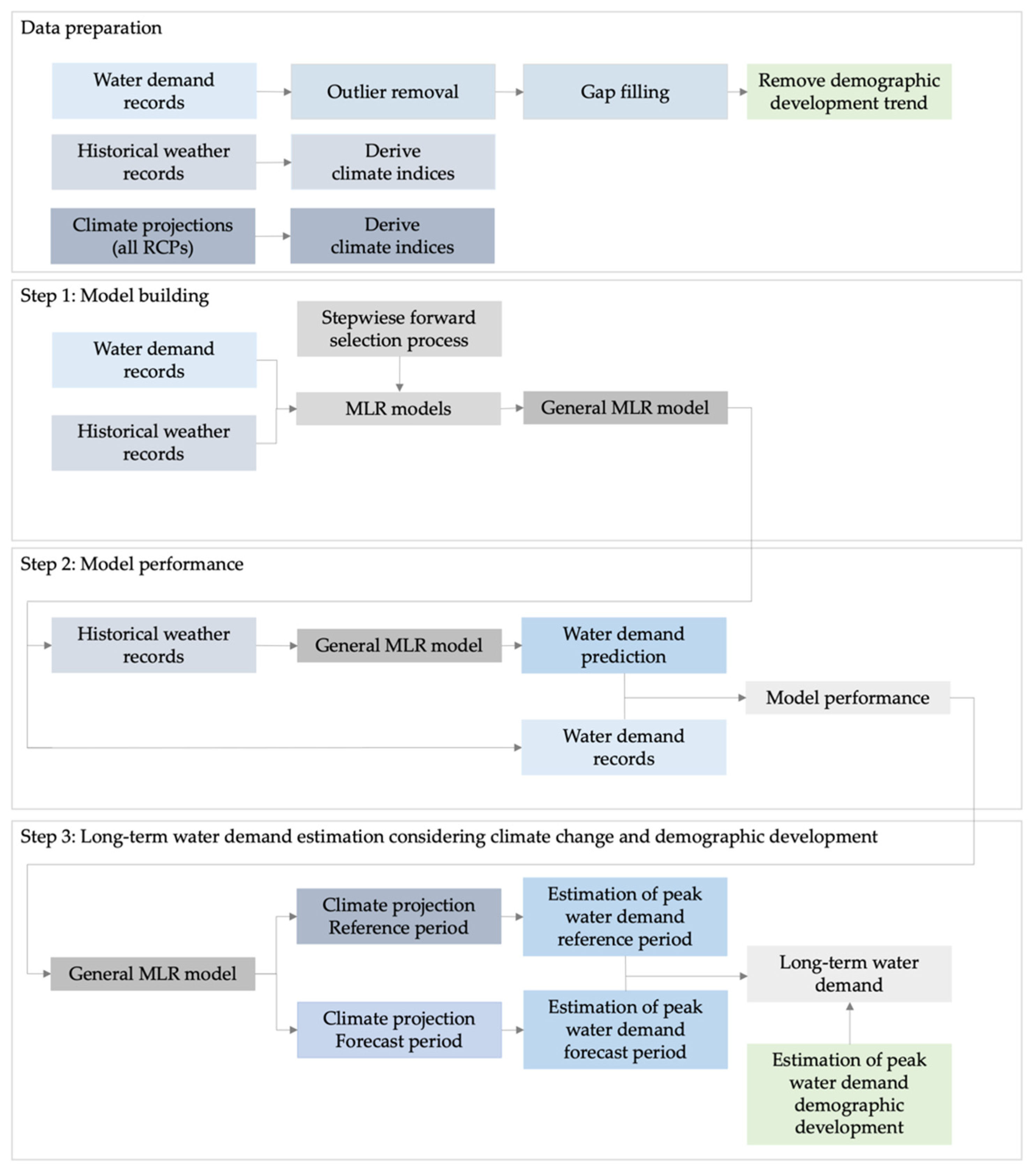
3.1. Data Preparation

The modeling process is preceded by intensive data preparation. Data preparation forms an important basis here, as it can influence the model performance and the results. For the study sites, several years of water demand records were available. Since the goal is to predict changes in the peak water demand, only water demand records where there were no system changes, such as merging two zones into one, during the recording period were used.
In the first step, an outlier removal was carried out to remove implausible peak and minimum demand values. The boxplot.stats [27] function in R (version 4.2.2) was used for outlier detection. All the outliers were removed, and linear interpolation was used to fill the gaps as there were only short gaps in all the zones. As population development has a major influence on the change in water demand, this trend was excluded from the measurement data. For this purpose, the increase in the water demand caused by the population increase was deducted from the measured data. The population trend is available for the individual years for each zone [28,29,30]. The population forecast is based on fertility, mortality, internal migration, external migration, and population status, such as age, gender, and origin. Cluster analyses were carried out, allowing regional types to be summarized. [31] Furthermore, the main variant of the current population forecast from STATISTIK AUSTRIA [32] was also taken into account. The multi-regional forecasting program SIKURS (Statistical information system for small-scale allocation and projection of a regional population structure) of the German KOSIS network was used for the calculation. [31] Since the population forecast is only available until 2050, the simple assumption was made that the population change will continue at the same rate until 2070.
Historical weather records were used in the model-building process. By using historical weather records, the correlation between climate indices and peak water demand can be analyzed. All the above-mentioned climate indices can be derived from the available weather records. This was performed to illustrate the correlation between climate indices and daily water demand and, subsequently, to estimate the change in water demand based on the change in climate indices. The data was prepared in the same way as in the previous study, and a detailed description can be found in the latter [10].

3.2. Model Building

As the MLR model proved to be suitable for water demand prediction [10], the existing modeling approach was extended in the present study.
The multiple linear regression aims to identify the relationship between a set of independent (X) and dependent variables (Y). The following equation represents the multiple linear regression [9].
Y = f X = β 0 + β 1 X 1 + β 2 X 2 + + β n X n + ϵ
Here, β 0 is the intercept. β n are the regression parameters for n independent variables, and ϵ represents the error term. In these models, the parameters β 0 , β 1 , …, β n have a linear relationship, meaning each parameter is multiplied by a variable X . These multiplication terms are added together to form the regression function [9].
In this step, the water demand records and the historical weather records were combined and a correlation analysis was performed to identify the variables to include in the model. The dataset was split into a training and a test dataset. To derive the significant climate indices (Section 2.2), general variables (days of the week and months), and combinations of variables, a stepwise forward variable selection [33] was performed during the modeling process. The days of the week were categorized from 1–7. Monday was used as the starting number; Sunday and public holidays were categorized in the same way. All the variables and combinations of variables were included in the model in the first step for the stepwise forward variable selection [33]. The Chi-square test was used to derive the significance (expressed by the p-value) for each variable and all the combinations. All the variables and combinations whose p-value was less than 0.1 were used to create an MLR model. The new p-values were then calculated and all the variables with a value greater than 0.1 were removed from the model. The goal was to derive a model that contained only variables and their combinations with a p-value < 0.1. This step was repeated until all the p-values were less than 0.1.
This step was carried out for each individual zone. Then, the individual models were compared with each other to derive all the variables that occurred in all the models. The final MRL model was created based on these variables.

3.3. Model Performance

In the second step, the model accuracy of the final model was checked. For this purpose, common measures of model accuracy were used, such as the mean absolute percentage error (MAPE) and the Pearson correlation (r). The following equations show the two measures [7]:
M A P E = 100 N t = 1 N Y t Y ^ t Y t
r = N ( Y t Y ^ t ) ( Y t ) ( Y ^ t ) N Y t 2 ( Y t ) 2 N Y ^ t 2 ( Y ^ t ) 2
The measurement and the forecast value for N time steps at time t are represented by Y t , and Y t ^ . Y t Y ^ t is the forecast error. MAPE is most suitable for comparing the model performance across different study sites as it is not influenced by the water capacity of the system [7]. Secondly, whether the peak demand was taken with sufficient accuracy was also assessed.

3.4. Long-Term Water Demand Estimation Considering Climate Change and Demographic Development

In the previous paper, the nearest grid box of the climate projections was selected for the supply system. In this study, the supply area was cut out of the climate projections, and all the grid boxes that lie within this boundary were summarized and the mean value was determined. When using climate projections, a long period must be selected to cover climate fluctuations. Therefore, a period of 20–30 years should be selected [23].
In this step, the MLR model was applied to the climate projections. There were 8 projections available for the RCP2.6 and 16 projections each for the RCP4.5 and RCP8.5. For this prediction, it is assumed that the water distribution system remains approximately the same for the periods under consideration. The water demand was determined for a reference period and two forecast periods.
In the final step, the change in the water demand caused by the population growth was considered. The population forecasts from [31] were used for this. This small-scale population forecast is available for Austria at the district level. In order to calculate the change in the water demand due to the population change, the percentage change in the water demand was calculated for each study site on the basis of the annual population change and the average water demand per person per day. Finally, we combined the change resulting from population growth with the change due to climate change.

4. Results and Discussion
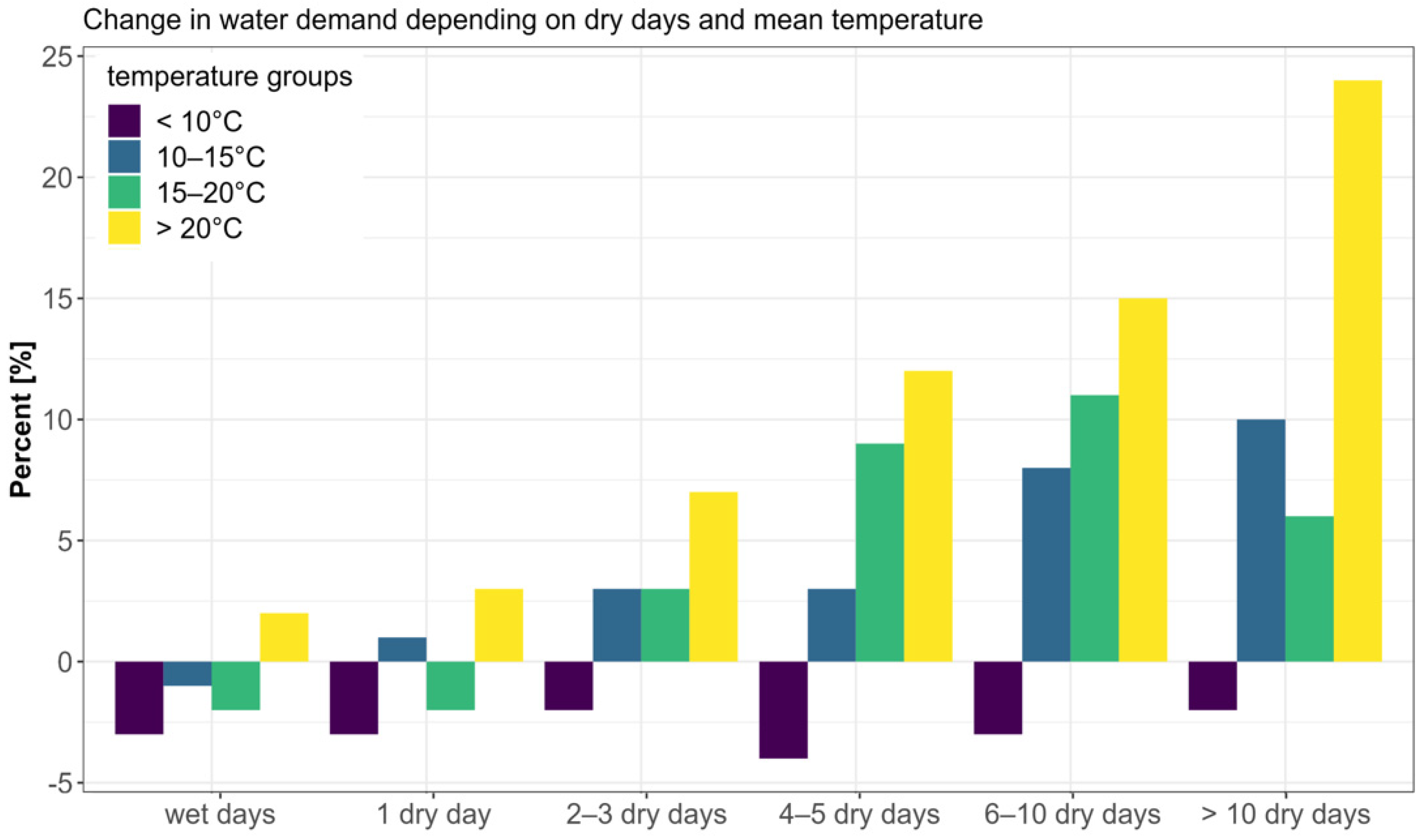
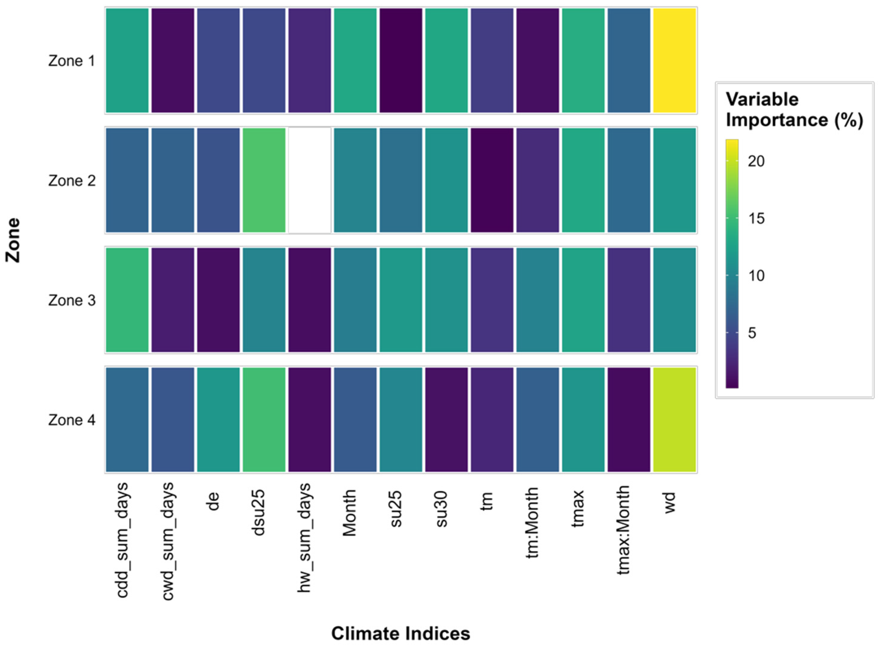
4.1. Model Building

First, an individual MLR model was derived for each zone. The time series was split into a training and test dataset for all the zones. Two-thirds of the time series was used to build and train the model and one-third of the time series was used to validate the model. The climate indices and the variables day of the week and the month were included in the modeling process. The significant variables and their combinations were determined using the stepwise forward variable selection process described in Section 3.2. The individual models were then compared to each other, and the variables that occurred in all the models were derived and a general MLR model was created. In all the study sites, the minimum temperature had no significant effect on the water demand. Some of the additional climate indices, such as dry hot days and dry heat waves, also showed no significance. However, the mean and maximum temperatures proved to be significant. Furthermore, the combination of the maximum temperature and month as well as the dry periods were kept in the model. Additionally, dry summer days showed significance in all the study sites. Hence, of the additional climate indices, the dry periods, the maximum temperature, and the dry summer days proved to be significant for water demand prediction. In the last study, heat waves could not be taken into account as no heat waves occurred during the short observation period. In this study, heat waves occurred in all the zones except Zone 2 during the observation period, so this climate index was taken into account. The individual variables used in the MLR model are listed below:
  • Mean temperature
  • Maximum temperature
  • Hot days
  • Summer days
  • Heat waves
  • Consecutive dry days
  • Consecutive wet days
  • Day of the week
  • Month
  • Dry summer days
  • Dry periods
  • Maximum temperature: month
  • Mean temperature: month
The variable importance was then evaluated for each zone and is shown in Figure 3. The color distribution represents the importance of the individual variables per zone. A brighter box indicates a higher importance of the variable in the zone. In Zone 2, the heat wave box (hw_sum_days) is white. This is because no heat waves occurred in this zone during the observation period.

4.2. Model Performance

The model accuracy was quantified using the metrics presented in Section 3.3. Since the previous paper found that the MLR model provides equivalent model results to common model approaches, a comparison between different model approaches is neglected in this paper. The results of the model accuracy tests for the training dataset are shown in Table 3. Good model accuracy was obtained for all the zones. The MAPE ranged from 4 and 9% for all the zones. Zone 1 had the best results. A satisfactory correlation was achieved for all the zones.
After the models were trained, the daily water demand was predicted using the test dataset. As with the training dataset, the model accuracy was determined. Table 4 shows the results of the model accuracy tests for the test dataset. The model also achieved good model accuracy here, but this was slightly worse than for the training dataset. The MAPE was between 5 and 11%. Zone 1 achieved very good results, with a MAPE of around 5%. The correlation was somewhat lower compared to the training dataset. Nevertheless, the results are satisfactory, with minor variations in the MAPE between the training and test datasets.
Whether the peak demand could be predicted with sufficient accuracy was also examined. Figure 4 shows the comparison between the measured data and the predicted water demand. The model reproduced the peaks for the training data well. For the test data, the model underestimated the peaks a little bit. Furthermore, the measured mean water demand was compared with the predicted mean water demand. The model slightly underestimates the water demand.
It can be clearly seen that good results were generated for all the zones. Furthermore, the influence of the climate indices on the model quality plays an important role when comparing the results with those of the previous study.

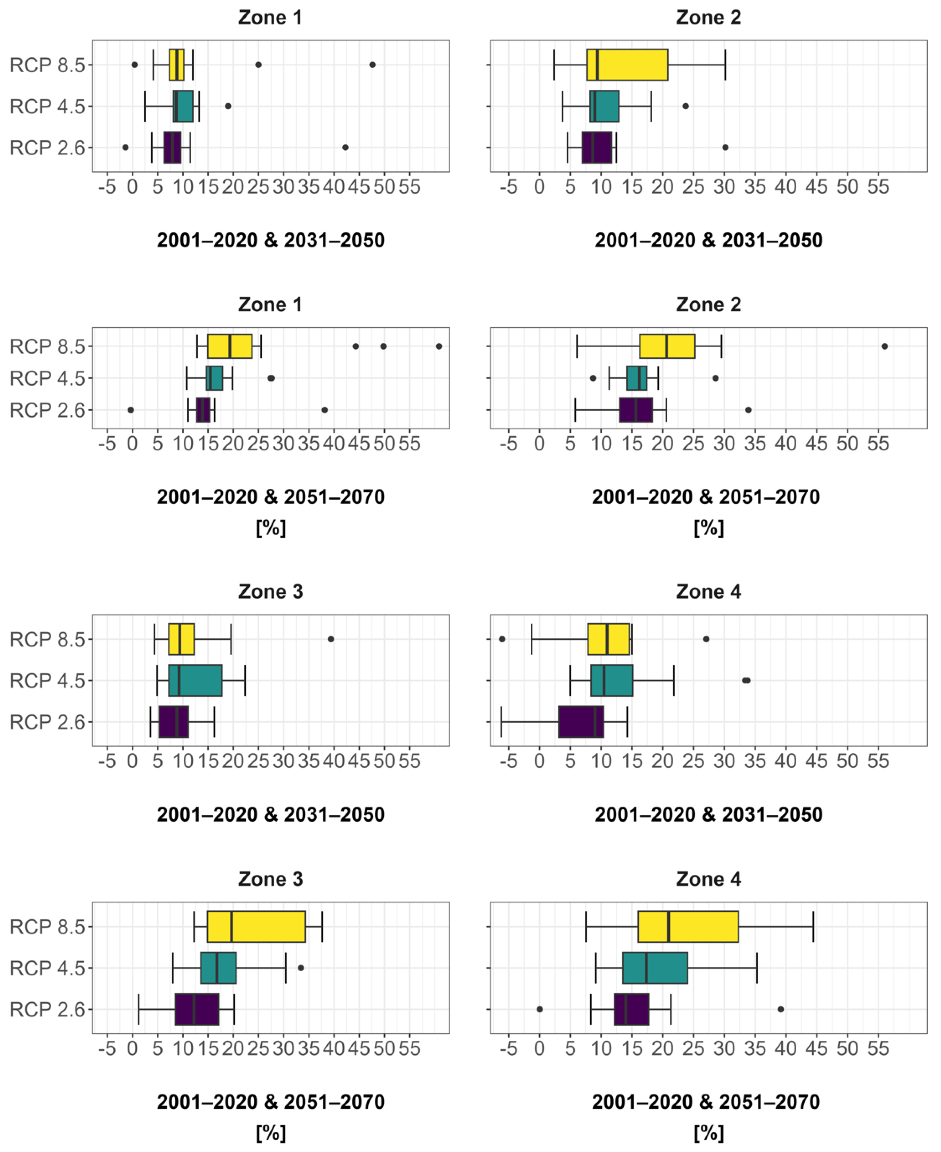
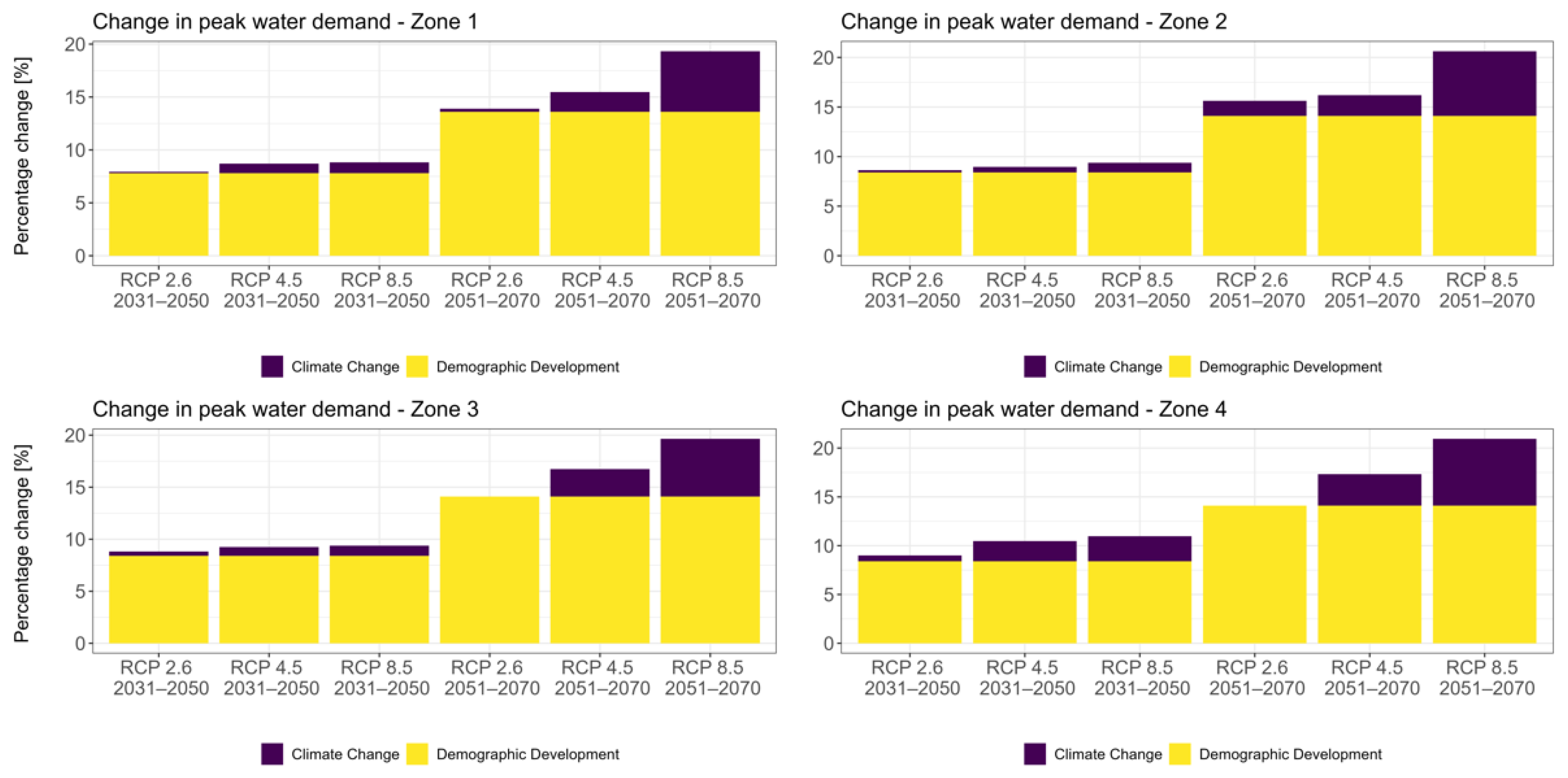
4.3. Long-Term Water Demand Estimation Considering Climate Change and Demographic Development

A reference period of 2001–2020 and two future periods, 2031–2050 and 2051–2070, were, therefore, selected for the projection. The three scenarios, RCP2.6, RCP4.5, and RCP8.5, were available for the prediction. The MLR model was used to predict the water demand for each individual climate projection. This resulted in a range of possible future water demands per zone. The water demand was predicted for the reference period and the future period and then compared to determine the change in the water demand. The change in the water demand was calculated as a percentage. Furthermore, the change in the water demand due to the changing population in the individual zones was included. An increase in the population was expected for all the zones. The development of the population was taken from the small-scale population forecast [31]. For this calculation, it was assumed that the average consumption per person and day remained approximately the same. The change in the water demand resulting from the population increase was combined with the change due to climate change.
Figure 5 shows the possible ranges of the future peak water demand due to climate change and demographic development. It is evident that the peak water demand varies with each climate change scenario. For the period 2031–2050, the change in the peak water demand does not yet fluctuate greatly due to the individual climate change scenarios. For all the zones, there is not much difference between the individual scenarios for this period. This may be due to the short distance between the reference period and the future period.
Additionally, a bar plot (Figure 6) was created to show the influence of climate change and population development more clearly. In the following figure, the change in the peak water demand due to climate change is shown in purple, and the change due to population development is shown in yellow. It is very clear that population development is the most significant factor in all the study sites. However, it should be noted that these results may be different for other study sites in Austria. An average change of around 8% may occur for RCP2.6 during the period 2031–2050. A possible average change of 9% is predicted for RCP4.5 and 9% for RCP8.5. Looking at the second period, 2051–2070, the results scatter more clearly between the individual scenarios. Here, it is easy to see that the water demand for the worst-case scenario, RCP8.5, can increase most significantly by 19%. For RCP4.5 the mean increase is 16%, and for RCP2.6, it is 14%.
From the results presented above, it can be deduced that the demand for water in the selected study sites in Austria will increase due to advancing climate change and population development. However, there is a difference between the individual climate change scenarios. Population development accounts for the most significant part of the change, but this can vary in other areas of Austria.

5. Conclusions

The aim of this study was to estimate the change in the peak water demand caused by climate change and demographic development. For this purpose, an MLR model was derived based on climate indices and variables, such as days of the week and the month. The model should be designed so that it can be easily applied to other zonal inflow data. The temperature-based indices, such as maximum temperature and summer days, were found to be particularly significant. We also found that the minimum temperature has no significance compared to the water demand. The model accuracy was assessed for the training and test datasets using common model quality parameters, such as the MAPE. Satisfactory results were obtained for all the selected zones. The MLR model slightly underestimated the water demand. This can be attributed to the fact that the increasing dry and hot periods are not yet adequately represented in the available data.
The MLR model was then applied to climate indices available from climate projections for the RCP2.6, RCP4.5, and RCP8.5. The peak water demand was predicted for a reference period, 2001–2020, as well as for two future periods, 2031–2050 and 2051–2070. The change in the peak water demand due to population growth was then calculated and combined with the previous change. An increase in the population is expected for all the study sites. For the first period, the results do not yet vary much between the different RCPs, which is in line with climate change assessments. For the second period, RCP2.6 predicts an average increase in the peak water demand of about 14%. However, only around 0.7% of this is due to climate change. For RCP4.5, 16% was predicted for the same period due to climate change and population growth for the study sites. On average, about 2.5% can be attributed to climate change. For RCP8.5, the predicted mean increase was 19% (around 6% due to climate change). It was found that for these study sites, the majority of the increase was due to population growth. However, in other parts of Austria, the results may be different due to different climatic conditions and population changes. Almost no increase in the water demand due to climate change was forecasted for RCP2.6, which underlines the importance of climate action [34]. To reduce the future increase in the water demand due to climate change, climate change adaptation measures should be further promoted. In particular, meeting the Sustainable Development Goals [35] should be a top priority to minimize the impact of climate change.
To improve the prediction, a scenario analysis of the individual study sites is recommended, in which different climate change scenarios and population developments are combined. Additionally, understanding the variations in the water demand among different consumer types at the building level would be valuable for estimating the impact of diverse urban development scenarios on water demand in the future. This may be important for future urban development to determine which neighborhoods will have the highest water demand based on the type of development. Furthermore, it is assumed that an analysis of the actual irrigation demand of private gardens and the exact water demand used for pool fillings would make the evaluations more accurate.

Author Contributions

Conceptualization, A.S. and D.F.-H.; methodology, A.S.; validation, A.S.; formal analysis, A.S.; investigation, A.S.; resources, D.F.-H.; data curation, A.S.; writing—original draft preparation, A.S.; writing—review and editing, A.S. and D.F.-H.; visualization, A.S.; supervision, D.F.-H.; project administration, D.F.-H.; funding acquisition, D.F.-H. All authors have read and agreed to the published version of the manuscript.

Funding

This research is part of the research project EWA funded by the Federal Ministry of Agriculture, Forestry, Regions and Water Management, with a funding amount of €190,000. (https://info.bml.gv.at/themen/wasser/nutzung-wasser/wasserversorgung/entscheidungshilfe-trinkwasserversorgung.html, accessed on 20 December 2023). Supported by the TU Graz Open Access Publishing Fund.

Data Availability Statement

The data presented in this study are available upon request from the corresponding author.

Acknowledgments

We sincerely wish to thank the water utilities for sharing their zonal inflow data. We would like to thank David Camhy and Reinhard Klingenberg for the detailed discussion and their support in evaluating the climate projections. We would also like to thank the reviewers for the helpful and constructive review comments that helped to improve this work significantly.

Conflicts of Interest

The authors declare no conflicts of interest. The funders had no role in the design of the study; in the collection, analysis, or interpretation of data; in the writing of the manuscript; or in the decision to publish the results.

References

  1. Dimkić, D. Temperature Impact on Drinking Water Consumption. Environ. Sci. Proc. 2020, 2, 31. [Google Scholar] [CrossRef]
  2. Wang, X.; Zhang, J.; Shahid, S.; Guan, E.; Wu, Y.; Gao, J.; He, R. Adaptation to Climate Change Impacts on Water Demand. Mitig. Adapt. Strateg. Glob. Chang. 2016, 21, 81–99. [Google Scholar] [CrossRef]
  3. Ashoori, N.; Dzombak, D.A.; Small, M.J. Modeling the Effects of Conservation, Demographics, Price, and Climate on Urban Water Demand in Los Angeles, California. Water Resour. Manag. 2016, 30, 5247–5262. [Google Scholar] [CrossRef]
  4. Murdock, S.H.; Albrecht, D.E.; Hamm, R.R.; Backman, K. Role of Sociodemographic Characteristics in Projections of Water Use. J. Water Resour. Plan. Manag. 1991, 117, 235–251. [Google Scholar] [CrossRef]
  5. Timotewos, M.T.; Barjenbruch, M.; Behailu, B.M. The Assessment of Climate Variables and Geographical Distribution on Residential Drinking Water Demand in Ethiopia. Water 2022, 14, 1722. [Google Scholar] [CrossRef]
  6. Neunteufel, R.; Richard, L.; Perfler, R. Wasserverbrauch und Wasserbedarf; Bundesministerium für Land- und Forstwirtschaft, Umwelt und Wasserwirtschaft: Wien, Austria, 2012.
  7. Donkor, E.A.; Mazzuchi, T.A.; Soyer, R.; Alan Roberson, J. Urban Water Demand Forecasting: Review of Methods and Models. J. Water Resour. Plan. Manag. 2014, 140, 146–159. [Google Scholar] [CrossRef]
  8. de Souza Groppo, G.; Costa, M.A.; Libânio, M. Predicting Water Demand: A Review of the Methods Employed and Future Possibilities. Water Supply 2019, 19, 2179–2198. [Google Scholar] [CrossRef]
  9. Adamowski, J.; Chan, H.; Prasher, S.; Ozga-Zielinski, B.; Sliusarieva, A. Comparison of Multiple Linear and Nonlinear Regression, Autoregressive Integrated Moving Average, Artificial Neural Network, and Wavelet Artificial Neural Network Methods for Urban Water Demand Forecasting in Montreal, Canada. Water Resour. Res. 2012, 48, 1528. [Google Scholar] [CrossRef]
  10. Stelzl, A.; Pointl, M.; Fuchs-Hanusch, D. Estimating Future Peak Water Demand with a Regression Model Considering Climate Indices. Water 2021, 13, 1912. [Google Scholar] [CrossRef]
  11. Adamowski, J. Peak Daily Water Demand Forecast Modeling Using Artificial Neural Networks. J. Water Resour. Plan. Manag. 2008, 134, 119–128. [Google Scholar] [CrossRef]
  12. Ghiassi, M.; Zimbra David, K.; Saidane, H. Urban Water Demand Forecasting with a Dynamic Artificial Neural Network Model. J. Water Resour. Plan. Manag. 2008, 134, 138–146. [Google Scholar] [CrossRef]
  13. Vonk, E.; Cirkel, D.G.; Blokker, M. Estimating Peak Daily Water Demand under Different Climate Change and Vacation Scenarios. Water 2019, 11, 1874. [Google Scholar] [CrossRef]
  14. Bakker, M.; van Duist, H.; van Schagen, K.; Vreeburg, J.; Rietveld, L. Improving the Performance of Water Demand Forecasting Models by Using Weather Input. Procedia Eng. 2014, 70, 93–102. [Google Scholar] [CrossRef]
  15. Donevska, K.; Panov, A. Climate Change Impact on Water Supply Demands: Case Study of the City of Skopje. Water Supply 2019, 19, 2172–2178. [Google Scholar] [CrossRef]
  16. Fiorillo, D.; Kapelan, Z.; Xenochristou, M.; De Paola, F.; Giugni, M. Assessing the Impact of Climate Change on Future Water Demand Using Weather Data. Water Resour. Manag. 2021, 35, 1449–1462. [Google Scholar] [CrossRef]
  17. Rasifaghihi, N.; Li, S.S.; Haghighat, F. Forecast of Urban Water Consumption under the Impact of Climate Change. Sustain. Cities Soc. 2020, 52, 101848. [Google Scholar] [CrossRef]
  18. GeoSphere Austria Data Hub. Available online: https://data.hub.geosphere.at/group/stationsdaten (accessed on 29 November 2023).
  19. Intergovernmental Panel on Climate Change (IPCC). Climate Change 2013—The Physical Science Basis: Working Group I Contribution to the Fifth Assessment Report of the Intergovernmental Panel on Climate Change; Cambridge University Press: Cambridge, UK, 2014; ISBN 978-1-107-05799-9. [Google Scholar]
  20. Moss, R.H.; Edmonds, J.A.; Hibbard, K.A.; Manning, M.R.; Rose, S.K.; van Vuuren, D.P.; Carter, T.R.; Emori, S.; Kainuma, M.; Kram, T.; et al. The next Generation of Scenarios for Climate Change Research and Assessment. Nature 2010, 463, 747–756. [Google Scholar] [CrossRef] [PubMed]
  21. Leuprecht, A.; Chimani, B.; Heinrich, G.; Hofstätter, M.; Kerschbaumer, M.; Kienberger, S.; Lexer, A.; Peßenteiner, S.; Poetsch, M.; Salzmann, M.; et al. OKS15 Bias Corrected EURO-CORDEX Models, 2nd ed.; CCCA Data Centre: Vienna, Austria; Available online: https://data.ccca.ac.at/group/oks15 (accessed on 20 December 2023).
  22. Mendlik, T.; Chimani, B.; Matulla, C.; Eitzinger, J.; Hiebl, J.; Hofstätter, M.; Kubu, G.; Maraun, D.; Schellander-Gorgas, T.; Thaler, S. STARC-Impact Bias Corrected ENSEMBLES, 1st ed.; CCCA Data Centre: Vienna, Austria; Available online: https://data.ccca.ac.at/group/starc-impact (accessed on 20 December 2023).
  23. Chimani, B.; Heinrich, G.; Hofstätter, M.; Kerschbaumer, M.; Kienberger, S.; Leuprecht, A.; Lexer, A.; Peßenteiner, S.; Poetsch, M.S.; Salzmann, M.; et al. and Truhetz, H. ÖKS15—Klimaszenarien für Österreich; Daten, Methoden Und Klimaanalyse; Federal Ministry Climate Action, Environment, Energy, Mobility, Innovation and Technology: Wien, Austria, 2016.
  24. Welcome|CCCA Data Server. Available online: https://data.ccca.ac.at/ (accessed on 4 November 2023).
  25. Jacob, D.; Petersen, J.; Eggert, B.; Alias, A.; Christensen, O.B.; Bouwer, L.M.; Braun, A.; Colette, A.; Déqué, M.; Georgievski, G.; et al. EURO-CORDEX: New High-Resolution Climate Change Projections for European Impact Research. Reg. Environ. Chang. 2014, 14, 563–578. [Google Scholar] [CrossRef]
  26. European Climate Assesment & Dataset Indices Dictionary. Available online: https://www.ecad.eu/indicesextremes/indicesdictionary.php#3 (accessed on 21 December 2023).
  27. DataCamp Boxplot. Stats: Box Plot Statistics. Available online: https://www.rdocumentation.org/packages/grDevices/versions/3.6.2/topics/boxplot.stats (accessed on 30 November 2023).
  28. Bevölkerung Stadtregion Wels|Stadtregionen. Available online: https://www.stadtregionen.at/wels/bev%C3%B6lkerung (accessed on 19 December 2023).
  29. Statistik Austria—Gemeinden. Available online: https://www.statistik.at/blickgem/gemDetail.do?gemnr=40301 (accessed on 19 December 2023).
  30. Statistiken der Landeshauptstadt Graz—Stadtportal der Landeshauptstadt Graz. Available online: https://www.graz.at/cms/beitrag/10104210/7749761/Statistiken_der_Landeshauptstadt_Graz.html (accessed on 19 December 2023).
  31. ÖROK-Regionalprognosen 2021–2050: Bevölkerung; Geschäftsstelle der Österreichischen Raumordnungskonferenz (ÖROK) (Ed.) Österreichische Raumordnungskonferenz: Wien, Austria, 2022; ISBN 978-3-9519791-5-1.
  32. Statistik Austria. Bevölkerungsprognosen für Österreich und Die Bundesländer. Available online: https://www.statistik.at/statistiken/bevoelkerung-und-soziales/bevoelkerung/demographische-prognosen/bevoelkerungsprognosen-fuer-oesterreich-und-die-bundeslaender (accessed on 30 October 2023).
  33. Gedefaw, M.; Hao, W.; Denghua, Y.; Girma, A. Variable Selection Methods for Water Demand Forecasting in Ethiopia: Case Study Gondar Town. Cogent Environ. Sci. 2018, 4, 1537067. [Google Scholar] [CrossRef]
  34. United Nations Climate Action. Available online: https://www.un.org/sustainabledevelopment/climate-action/ (accessed on 30 November 2023).
  35. United Nations Take Action for the Sustainable Development Goals. Available online: https://www.un.org/sustainabledevelopment/sustainable-development-goals/ (accessed on 30 November 2023).
Figure 1. Change in water demand depending on dry days and mean temperature.
Water 16 00127 g001
Figure 2. Model building workflow. The first step is data preparation. The modeling process is divided into three steps. The first is model building, the second is model performance assessment, and the final step is long-term peak water demand estimation.
Water 16 00127 g002
Figure 3. Variable importance MLR model for each zone. The color gradations represent the variable importance of the MLR model. The brighter the box the more important the variable is.
Water 16 00127 g003
Figure 4. Example of the comparison of the measured water demand (thick purple line) and the predicted water demand (thin green line) for the training dataset (left) and for the test data (right) for Zone 1 and one year.
Water 16 00127 g004
Figure 5. Increase in peak water demand due to climate change and demographic development. The percentage change in peak water demand between the reference period and future periods is shown.
Water 16 00127 g005
Figure 6. Average change in peak water demand due to climate change and demographic development. The change due to climate change is the purple part and the yellow part shows the change due to demographic development.
Water 16 00127 g006
Table 1. Significant climate indices adapted from [23,26].
Climate Indices AbbreviationDescription
Air temperature (°C)tmMean temperature [23]
Hot days (days)su30Days with a maximum temperature of more than 30.0 °C [23]
Summer days (days)su25Days with a maximum temperature of more than 25.0 °C [23,26]
Heat waves (days)hw_sum_daysA period of at least three days with a daily maximum temperature of more than 30.0 °C and a daily minimum temperature of at least 18.0 °C [23]
Consecutive dry days (days)cdd_sum_daysAn episode lasting at least five days with a precipitation amount of less than 1 mm [23,26]
Consecutive wet days (days)cwd_sum_daysAn episode lasting at least three days with a precipitation amount of at least 1 mm [23,26]
Table 2. New climate indices.
Climate Indices AbbreviationDescription
Maximum air temperature (°C)tmaxMaximum temperature
Minimum air temperature (°C)tminMinimum temperature
Dry hot days (days)dsu30Days with a maximum temperature of more than 30.0 °C and a precipitation amount of less than 1 mm
Dry summer days (days)dsu25Days with a maximum temperature of more than 25.0 °C and a precipitation amount of less than 1 mm
Dry heat waves (days)dhwA period of at least three days with a daily maximum temperature of more than 30.0 °C and a daily minimum temperature of less than 18.0 °C and a precipitation amount of less than 1 mm
Dry period (days)deAn episode that is only interrupted if there is more than 1 mm of precipitation on three consecutive days.
Table 3. Model accuracy for the training data set for all zones.
ZoneMAPE (%)r (-)
Zone 14.40.78
Zone 2 8.10.69
Zone 38.90.62
Zone 49.00.71
Table 4. Model accuracy for the test dataset for all zones.
ZoneMAPE (%)r (-)
Zone 14.70.78
Zone 2 8.90.69
Zone 38.90.54
Zone 410.60.52
Disclaimer/Publisher’s Note: The statements, opinions and data contained in all publications are solely those of the individual author(s) and contributor(s) and not of MDPI and/or the editor(s). MDPI and/or the editor(s) disclaim responsibility for any injury to people or property resulting from any ideas, methods, instructions or products referred to in the content.

