
Research on Downstream Safety Risk Warning Model for Small Reservoirs Based on Granger Probabilistic Radial Basis Function Neural Network

Abstract
:1. Introduction
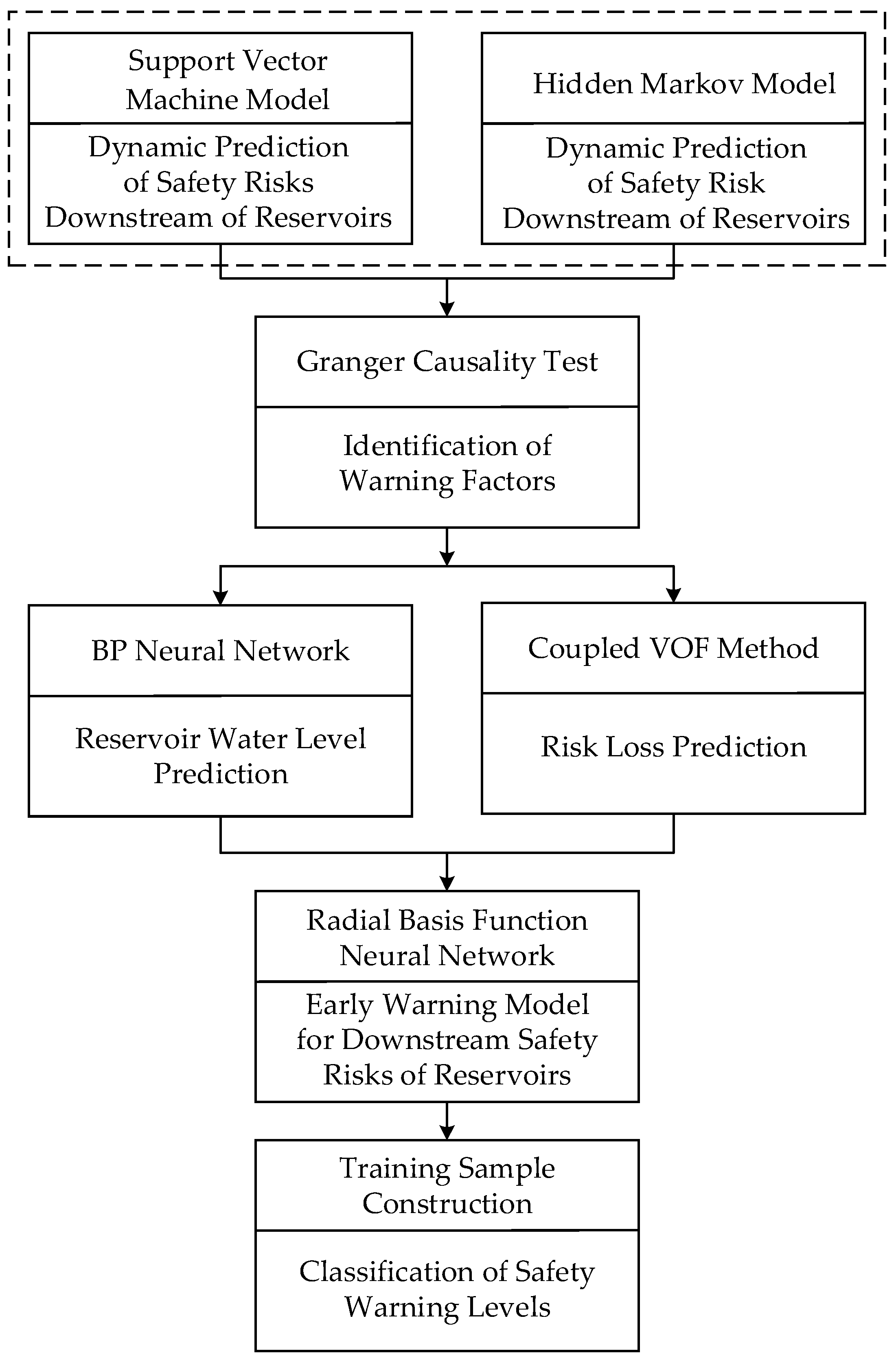
2. Research Ideas
3. Research Design
3.1. Analysis of Safety Risk Warning Factors Based on Granger Causality Test
3.1.1. Factor Identification Method Based on Granger Causality Test
3.1.2. Analysis of Early Warning Factors for Downstream Safety Risks in Small Reservoirs
3.2. Construction of Downstream Safety Early Warning Model for Small Reservoirs Based on Neural Network
3.2.1. Construction of BP Neural Network for Reservoir Level
3.2.2. Construction of Three-Dimensional Two-Equation Model Using VOF Method for Risk Loss
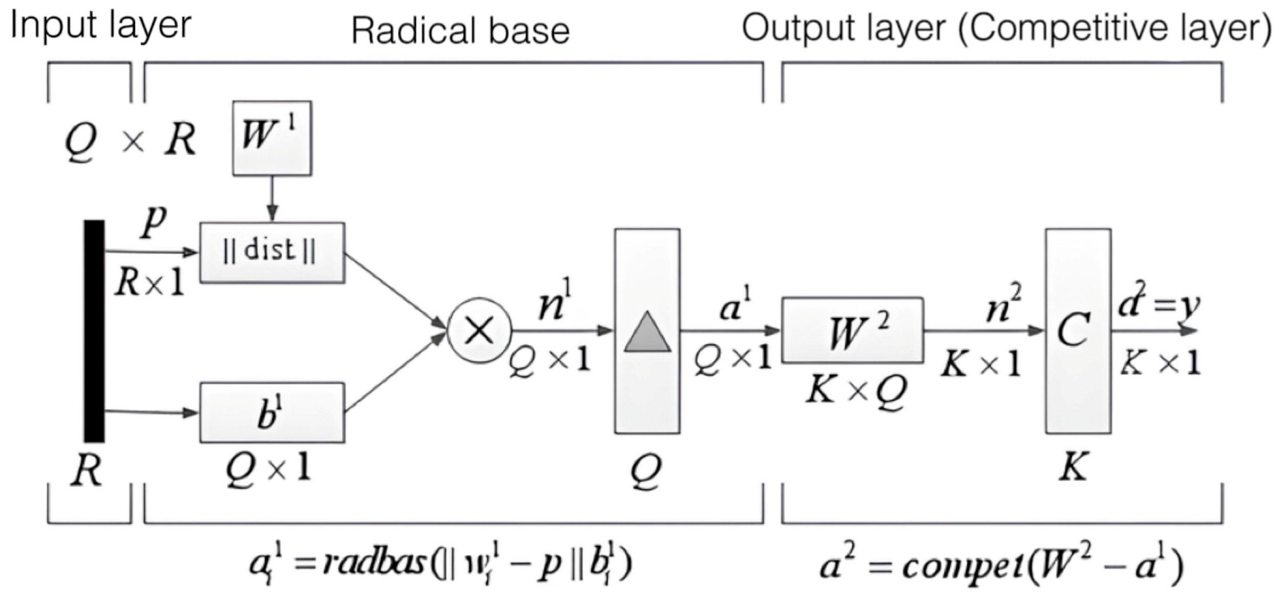
3.2.3. Construction of Probabilistic Radial Basis Neural Network for Risk Early Warning
4. Example Analyses
4.1. Case Background
4.2. J Reservoir Inflow Forecast
- (1)
- Observational Data Smoothness Test
- (2)
- Causality Tests for Variables
- (3)
- Granger Test for the Variable
- (4)
- Data Accuracy Check
- (5)
- Evaluation of the J Reservoir Inflow Prediction Results
4.3. J Prediction of Risk Level Downstream of J Reservoir
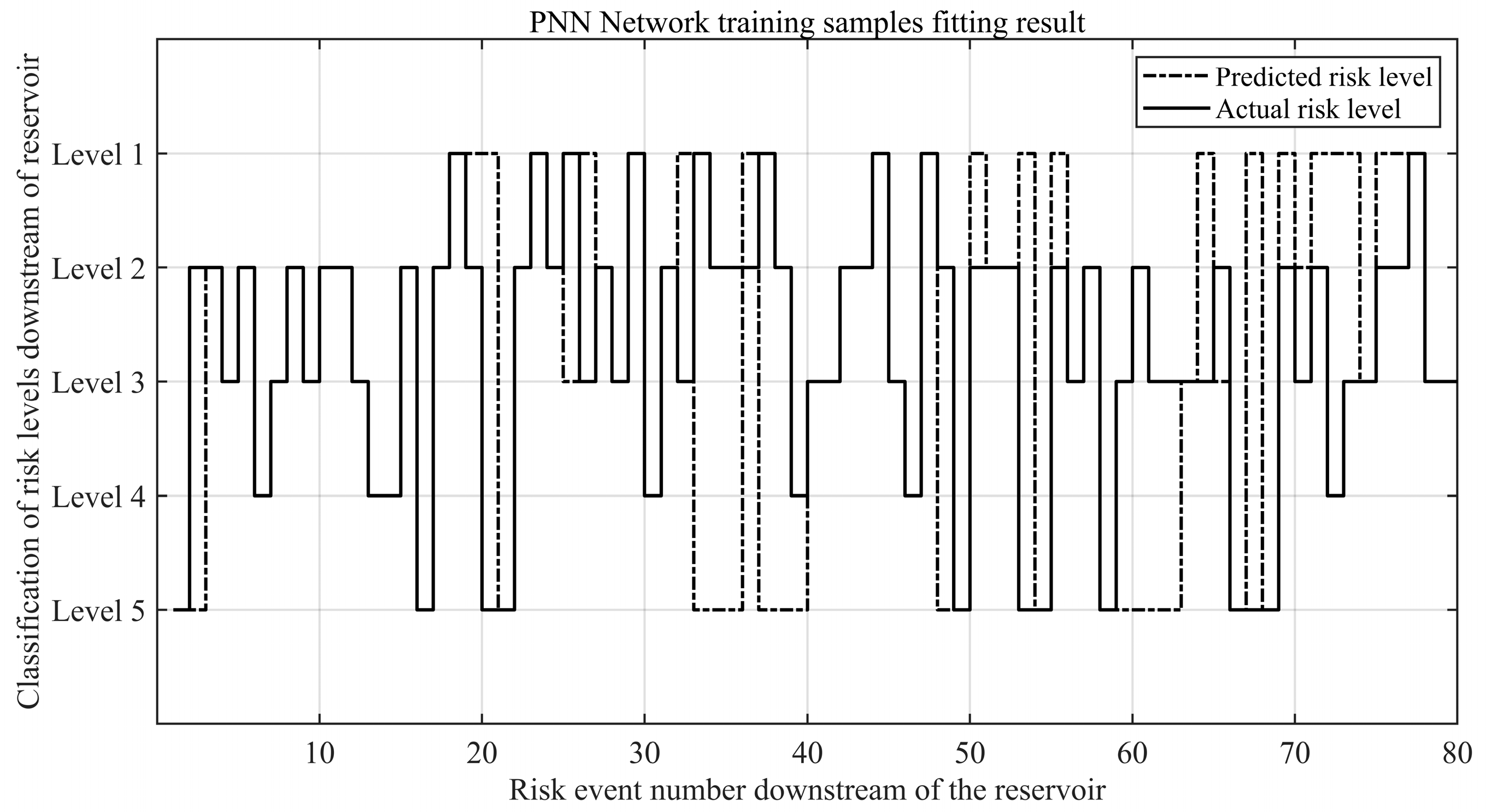
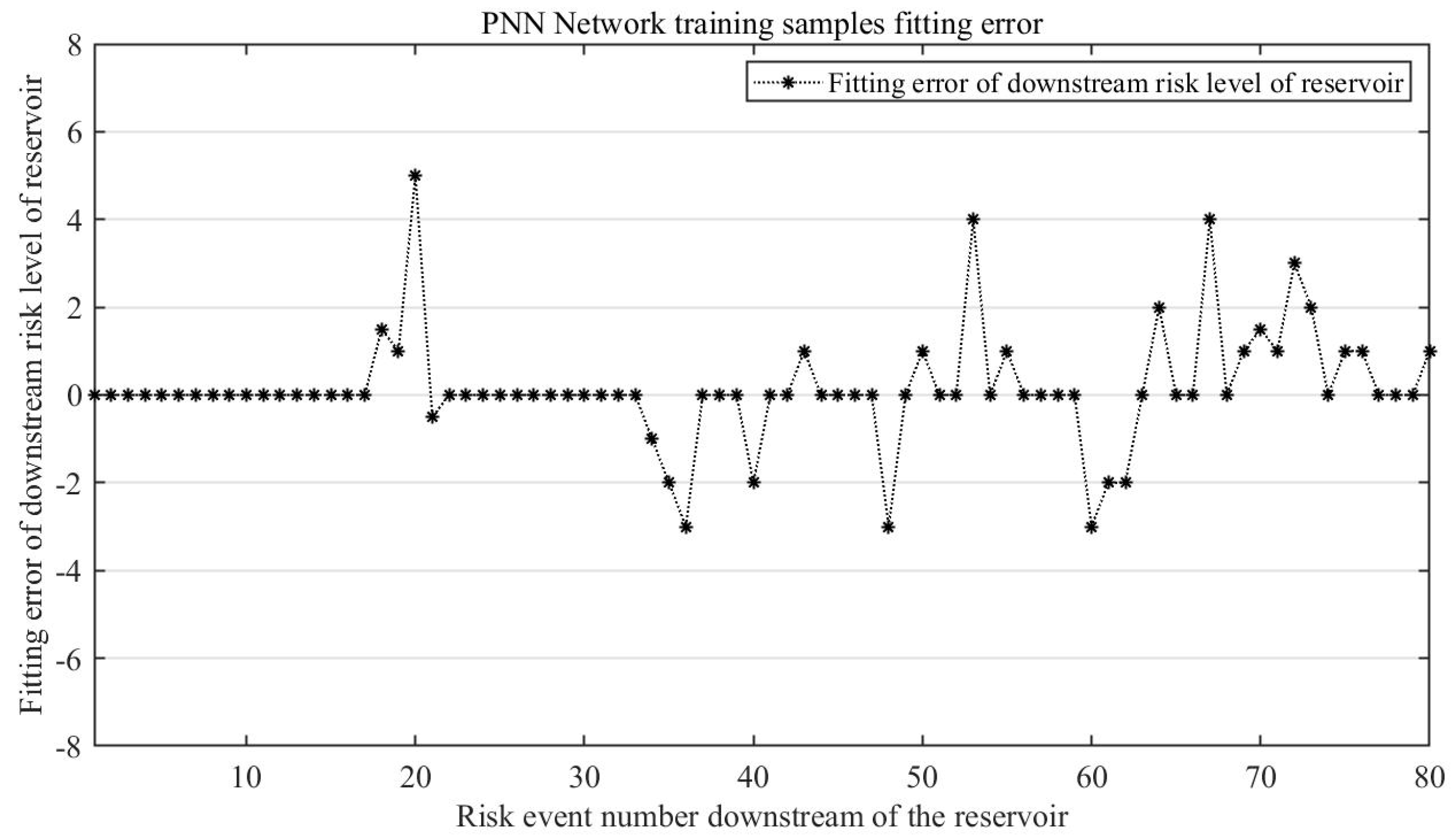
4.3.1. Analysis of Risk Level Prediction Process Downstream of J Reservoir
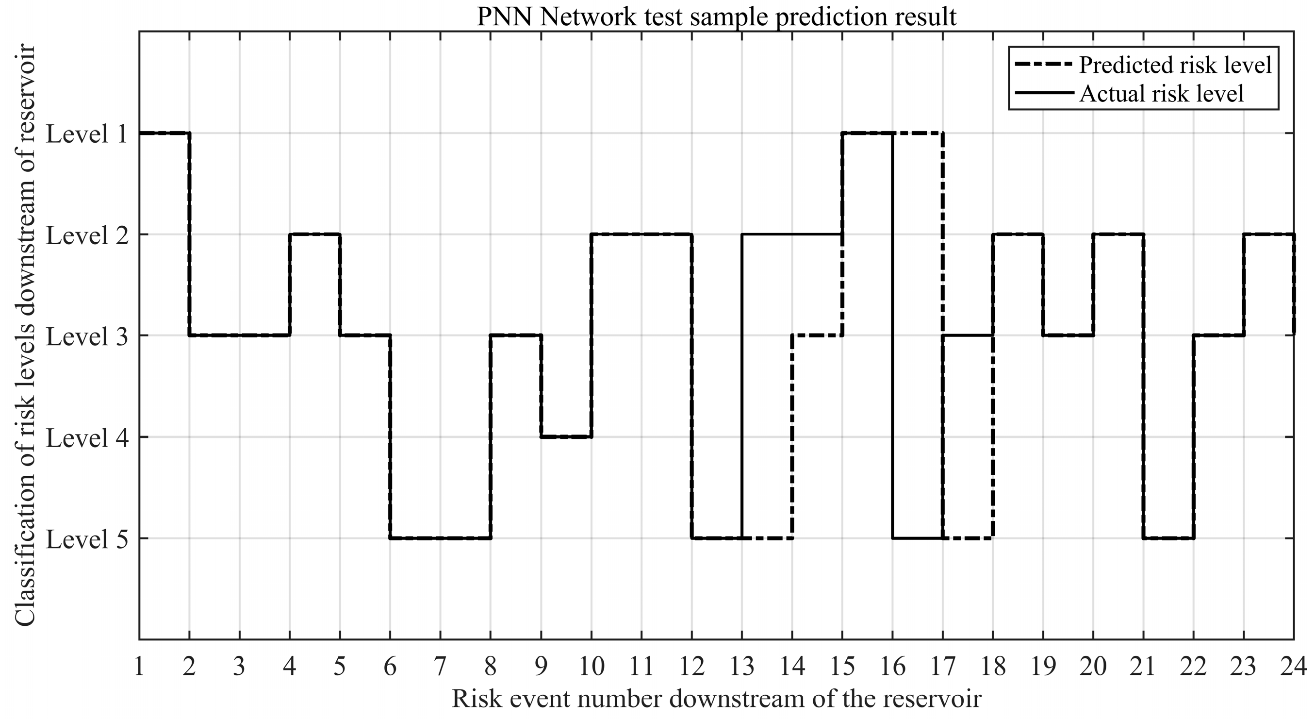
4.3.2. Analysis of the Prediction Results for Risk Levels of Downstream of J Reservoir
5. Conclusions
Author Contributions
Funding
Data Availability Statement
Conflicts of Interest
References
- Hall, J.; Arheimer, B.; Borga, M.; Brázdil, R.; Claps, P.; Kiss, A.; Kjeldsen, T.R.; Kriaučiūnienė, J.; Kundzewicz, Z.W.; Lang, M.; et al. Understanding flood regime changes in Europe: A state-of-the-art assessment. Hydrol. Earth Syst. Sci. 2014, 18, 2735–2772. [Google Scholar] [CrossRef]
- Gabriel-Martin, I.; Sordo-Ward, A.; Santillán, D.; Garrote, L. Flood Control Versus Water Conservation in Reservoirs: A New Policy to Allocate Available Storage. Water 2020, 12, 994. [Google Scholar] [CrossRef]
- Hou, T.S.; Xu, G.L.; Zhang, D.Q.; Liu, H.Y. Stability analysis of Gongjiacun landslide in the three Gorges Reservoir area under the action of reservoir water level fluctuation and rainfall. Nat. Hazards 2022, 114, 1647–1683. [Google Scholar] [CrossRef]
- Yussouf, N.; Wilson, K.A.; Martinaitis, S.M.; Vergara, H.; Heinselman, P.L.; Gourley, J.J. The Coupling of NSSL Warn-on-Forecast and FLASH Systems for Probabilistic Flash Flood Prediction. J. Hydrometeorol. 2020, 21, 123–141. [Google Scholar] [CrossRef]
- Won, Y.-M.; Lee, J.-H.; Moon, H.-T.; Moon, Y.-I. Development and Application of an Urban Flood Forecasting and Warning Process to Reduce Urban Flood Damage: A Case Study of Dorim River Basin, Seoul. Water 2022, 14, 187. [Google Scholar] [CrossRef]
- Li, W.; Lin, K.; Zhao, T.; Lan, T.; Chen, X.; Du, H.; Chen, H. Risk assessment and sensitivity analysis of flash floods in ungauged basins using coupled hydrologic and hydrodynamic models. J. Hydrol. 2019, 572, 108–120. [Google Scholar] [CrossRef]
- Ma, M.; Wang, H.; Yang, Y.; Zhao, G.; Tang, G.; Hong, Z.; Hong, Y. Development of a new rainfall-triggering index of flash flood warning-case study in Yunnan province, China. J. Flood Risk Manag. 2021, 14, e126761. [Google Scholar] [CrossRef]
- Mohanty, A.; Hussain, M.; Mishra, M.; Kattel, D.B.; Pal, I. Exploring community resilience and early warning solution for flash floods, debris flow and landslides in conflict prone villages of Badakhshan, Afghanistan. Int. J. Disaster Risk Reduct. 2019, 33, 5–15. [Google Scholar] [CrossRef]
- Hardy, J.; Gourley, J.J.; Kirstetter, P.-E.; Hong, Y.; Kong, F.; Flamig, Z.L. A method for probabilistic flash flood forecasting. J. Hydrol. 2016, 541, 480–494. [Google Scholar] [CrossRef]
- Corral, C.; Berenguer, M.; Sempere-Torres, D.; Poletti, L.; Silvestro, F.; Rebora, N. Comparison of two early warning systems for regional flash flood hazard forecasting. J. Hydrol. 2019, 572, 603–619. [Google Scholar] [CrossRef]
- Yuan, W.; Lu, L.; Song, H.; Zhang, X.; Xu, L.; Su, C.; Liu, M.; Yan, D. Study on the early warning for flash flood based on random rainfall pattern. Water Resour. Manag. 2022, 36, 1587–1609. [Google Scholar] [CrossRef]
- Talei, A.; Chua LH, C.; Quek, C. A novel application of a neuro-fuzzy computational technique in event-based rainfall–runoff modeling. Expert Syst. Appl. 2010, 37, 7456–7468. [Google Scholar] [CrossRef]
- Feng, K.; Zhou, J.; Liu, Y.; Lu, C. Hydrological uncertainty processor (HUP) with estimation of the marginal distribution by a Gaussian mixture model. Water Resour. Manag. 2019, 33, 2975–2990. [Google Scholar] [CrossRef]
- Li, Q.; Wang, Y.; Li, H.; Zhang, M.; Li, C.; Chen, X. Research on rainfall early warning indicators of flash flood disasters based on flood peak modulus. J. Earth Inf. Sci. 2017, 12, 1643–1652. [Google Scholar]
- Yussouf, N.; Knopfmeier, K.H. Application of the Warn-on-Forecast system for flash-flood-producing heavy convective rainfall events. Q. J. R. Meteorol. Soc. 2019, 145, 2385–2403. [Google Scholar] [CrossRef]
- Lin, K.; Chen, H.; Xu, C.Y.; Yan, P.; Lan, T.; Liu, Z.; Dong, C. Assessment of flash flood risk based on improved analytic hierarchy process method and integrated maximum likelihood clustering algorithm. J. Hydrol. 2020, 584, 124696. [Google Scholar] [CrossRef]
- Zhou, Y.; Wu, Z.; Xu, H.; Wang, H. Prediction and early warning method of inundation process at waterlogging points based on Bayesian model average and data-driven. J. Hydrol. Reg. Stud. 2022, 44, 101248. [Google Scholar] [CrossRef]
- Jodar-Abellan, A.; Valdes-Abellan, J.; Pla, C.; Gomariz-Castillo, F. Impact of land use changes on flash flood prediction using a sub-daily SWAT model in five Mediterranean ungauged watersheds (SE Spain). Sci. Total Environ. 2019, 657, 1578–1591. [Google Scholar] [CrossRef]
- Satriagasa, M.C.; Tongdeenok, P.; Kaewjampa, N. Assessing the Implication of Climate Change to Forecast Future Flood Using SWAT and HEC-RAS Model under CMIP5 Climate Projection in Upper Nan Watershed, Thailand. Sustainability 2023, 15, 5276. [Google Scholar] [CrossRef]
- Costache, R.; Bui, D.T. Identification of areas prone to flash-flood phenomena using multiple-criteria decision-making, bivariate statistics, machine learning and their ensembles. Sci. Total Environ. 2020, 712, 136492. [Google Scholar] [CrossRef]
- Panahi, M.; Jaafari, A.; Shirzadi, A.; Shahabi, H.; Rahmati, O.; Omidvar, E.; Bui, D.T. Deep learning neural networks for spatially explicit prediction of flash flood probability. Geosci. Front. 2021, 12, 101076. [Google Scholar] [CrossRef]
- Bui, D.T.; Ngo, P.T.T.; Pham, T.D.; Jaafari, A.; Minh, N.Q.; Hoa, P.V.; Samui, P. A novel hybrid approach based on a swarm intelligence optimized extreme learning machine for flash flood susceptibility mapping. CATENA 2019, 179, 184–196. [Google Scholar] [CrossRef]
- Xu, C.; Yang, J.; Wang, L. Application of Remote-Sensing-Based Hydraulic Model and Hydrological Model in Flood Simulation. Sustainability 2022, 14, 8576. [Google Scholar] [CrossRef]
- Bahramian, K.; Nathan, R.; Western, A.W.; Ryu, D. Towards an Ensemble-based Short-term Flood Forecasting Using an Event-based Flood Model—Incorporating Catchment-average Estimates of Soil Moisture. J. Hydrol. 2020, 593, 125828. [Google Scholar] [CrossRef]
- Al-Amri, N.S.; Ewea, H.A.; Elfeki, A.M. Stochastic Rational Method for Estimation of Flood Peak Uncertainty in Arid Basins: Comparison between Monte Carlo and First Order Second Moment Methods with a Case Study in Southwest Saudi Arabia. Sustainability 2023, 15, 4719. [Google Scholar] [CrossRef]
- Yudianto, D.; Ginting, B.M.; Sanjaya, S.; Rusli, S.R.; Wicaksono, A. A Framework of Dam-Break Hazard Risk Mapping for a Data-Sparse Region in Indonesia. ISPRS Int. J. Geo-Inf. 2021, 10, 110. [Google Scholar] [CrossRef]
- Zhenghua, L. Application and Efficiency of Probabilistic Neural Network in Suspicious Transaction Surveillance. In Proceedings of the 2015 Seventh International Conference on Measuring Technology and Mechatronics Automation, Nanchang, China, 13–14 June 2015; IEEE: Piscataway, NJ, USA, 2015; pp. 178–181. [Google Scholar]
- Luo, Y.; Dong, Z.; Liu, Y.; Wang, X.; Shi, Q.; Han, Y. Research on stage-divided water level prediction technology of rivers-connected lake based on machine learning: A case study of Hongze Lake, China. Stoch. Environ. Res. Risk Assess. 2021, 35, 2049–2065. [Google Scholar] [CrossRef]
- Granger, C.W.J. Investigating Causal Relations by Econometric Models and Cross-Spectral Methods. Econometrica 1969, 37, 424–438. [Google Scholar] [CrossRef]
- Pastor, D.J.; Fullerton, T.M., Jr. Municipal Water Consumption and Urban Economic Growth in El Paso. Water 2020, 12, 2656. [Google Scholar] [CrossRef]
- Liu, Z.; Guo, S.; Guo, J.; Liu, P. The impact of Three Gorges Reservoir refill operation on water levels in Poyang Lake, China. Stoch. Environ. Res. Risk Assess. 2017, 31, 879–891. [Google Scholar] [CrossRef]
- Liu, H.; Zhou, G.; Zhou, Y.; Huang, H.; Wei, X. An RBF neural network based on improved black widow optimization algorithm for classification and regression problems. Front. Neuroinform. 2023, 16, 1103295. [Google Scholar] [CrossRef]
- Li, J.; Ni, Z.; Zhu, X.; Xu, Y. Drought prediction model based on parallel integrated learning of best-point firefly algorithm and BP neural network. Syst. Eng.-Theory Pract. 2018, 38, 1343–1353. [Google Scholar]
- Feng, G.; Cui, D.; Zhang, Q.; Dai, X. Application of neural network-assisted multi-objective particle swarm optimization algorithm in complex product design. J. Syst. Manag. 2019, 28, 687–696+707. [Google Scholar] [CrossRef]
- Fernández-Nóvoa, D.; García-Feal, O.; González-Cao, J.; de Gonzalo, C.; Rodríguez-Suárez, J.A.; Ruiz del Portal, C.; Gómez-Gesteira, M. MIDAS: A New Integrated Flood Early Warning System for the Miño River. Water 2020, 12, 2319. [Google Scholar] [CrossRef]
- Hussein, S.; Abdelkareem, M.; Hussein, R.; Askalany, M. Using remote sensing data for predicting potential areas to flash flood hazards and water resources. Remote Sens. Appl. Soc. Environ. 2019, 16, 100254. [Google Scholar] [CrossRef]
- Li, S.; Jiang, Q.; Xu, Y.; Feng, K.; Wang, Y.; Sun, B.; Yan, X.; Sheng, X.; Zhang, K.; Ni, Q. Digital twin-driven focal modulation-based convolutional network for intelligent fault diagnosis. Reliab. Eng. Syst. Saf. 2023, 240, 109590. [Google Scholar] [CrossRef]
- Standardization Administration of China. Hydrological Information Specification. November 2008. Available online: https://openstd.samr.gov.cn/bzgk/gb/newGbInfo?hcno=9A1A51DA9FAD3B785C239A1FC2C5CAF3 (accessed on 24 November 2023).


| Level 1 | Level 2 | Level 3 | Level 4 | Level 5 | |
|---|---|---|---|---|---|
| R1 Alarm time/(h) | [0, 450] | [450, 525] | [525, 600] | [600, 675] | [675, 750] |
| R2 Average annual rainfall/(mm) | [0, 0.2] | [0.2, 0.8] | [0.8, 1.4] | [1.4, 2.0] | [2.0, 2.5] |
| R3 Depth of inundation/(m) | [0, 0.6] | [0.6, 1.2] | [1.2, 1.8] | [1.8, 2.4] | [2.4, 10] |
| R4 Flood velocity/(m3·s−1) | [0.25, 0.75] | [0.75, 1.75] | [1.75, 2.75] | [2.75, 3.75] | [3.75, 5.0] |
| R5 Population density at risk/(people·km−2) | [0, 100] | [100, 225] | [225, 350] | [350, 475] | [475, 600] |
| R6 Unit area GDP(/ten thousand yuan·km−2) | [0, 100] | [100, 300] | [300, 500] | [500, 700] | [700, 2000] |
| R7 Agricultural output intensity/(ten thousand yuan·km−2) | [0, 20] | [20, 80] | [80, 140] | [140, 200] | [200, 250] |
| R8 Density of commercial and industrial property in communes/(ten thousand yuan·km−2) | [0, 100] | [100, 500] | [500, 900] | [900, 1300] | [1300, 2000] |
| R9 Density of traffic arteries/(km·km−2) | [0, 0.2] | [0.2, 0.6] | [0.6, 1.0] | [1.0, 11.4] | [1.4, 2.0] |
| Evaluation Level | Characteristics Status | Characteristics |
|---|---|---|
| Level 1 | Slight risk | Flooding is less likely to occur, and the area subject to flooding is less economically developed than the surrounding area. |
| Level 2 | Average Risk | The likelihood of flooding is low, and the economic development of the affected area is slightly below the general level of the local area. |
| Level 3 | Medium Risk | The likelihood of flooding is moderate, and the economic development of the affected area is at a moderate level for the region. |
| Level 4 | High Risk | The likelihood of flooding is high and the economic development of the affected area is above the local average. |
| Level 5 | Heavy Risk | Higher likelihood of flooding and higher level of economic development in the affected area than in the surrounding area. |
| Variable | Null Hypothesis | t-Statistic | t Critical Values 1% | t Critical Values 5% | t Critical Values 10% | p Value | Conclusion |
|---|---|---|---|---|---|---|---|
| has a unit root | −30.31612 | −2.566212 | −1.940993 | −1.616586 | 0.0002 | stationary | |
| has a unit root | −5.045221 | −3.433736 | −2.862920 | −2.567552 | 0.0000 | stationary | |
| has a unit root | −3.671521 | −3.433732 | −2.862922 | −2.567552 | 0.0001 | stationary | |
| has a unit root | −3.634508 | −2.566215 | −1.940994 | −1.616583 | 0.0004 | stationary |
| Excluded | Chi-sq | df | Prob. | Conclusion (t Critical Values 5%) |
|---|---|---|---|---|
| 0.186633 | 2 | 0.3641 | Accepted | |
| 6.252843 | 2 | 0.0424 | ||
| 0.649981 | 2 | 0.9389 | Accepted |
| Null Hypothesis: | Obs | F-Statistic | Prob. |
|---|---|---|---|
| does not Granger Cause | 1836 | 1.39385 | 0.0948 |
| does not Granger Cause | 1.74287 | 0.0163 |
| Prediction Stage | Predict Results before Data Filtering | Prediction Results after Data Filtering |
|---|---|---|
| Conformity rate/% | 24.99 | 45.78 |
| Average relative error level/% | 39.11 | 21.50 |
| Average error level/(m3/s) | 629.55 | 387.41 |
| Nash–Sutcliffe Efficiency | 0.34 | 0.67 |
Disclaimer/Publisher’s Note: The statements, opinions and data contained in all publications are solely those of the individual author(s) and contributor(s) and not of MDPI and/or the editor(s). MDPI and/or the editor(s) disclaim responsibility for any injury to people or property resulting from any ideas, methods, instructions or products referred to in the content. |
© 2023 by the authors. Licensee MDPI, Basel, Switzerland. This article is an open access article distributed under the terms and conditions of the Creative Commons Attribution (CC BY) license (https://creativecommons.org/licenses/by/4.0/).
Share and Cite
Xue, S.; Chen, J.; Li, S.; Huang, H. Research on Downstream Safety Risk Warning Model for Small Reservoirs Based on Granger Probabilistic Radial Basis Function Neural Network. Water 2024, 16, 130. https://doi.org/10.3390/w16010130
Xue S, Chen J, Li S, Huang H. Research on Downstream Safety Risk Warning Model for Small Reservoirs Based on Granger Probabilistic Radial Basis Function Neural Network. Water. 2024; 16(1):130. https://doi.org/10.3390/w16010130
Chicago/Turabian StyleXue, Song, Jingyan Chen, Sheng Li, and Huaai Huang. 2024. "Research on Downstream Safety Risk Warning Model for Small Reservoirs Based on Granger Probabilistic Radial Basis Function Neural Network" Water 16, no. 1: 130. https://doi.org/10.3390/w16010130
APA StyleXue, S., Chen, J., Li, S., & Huang, H. (2024). Research on Downstream Safety Risk Warning Model for Small Reservoirs Based on Granger Probabilistic Radial Basis Function Neural Network. Water, 16(1), 130. https://doi.org/10.3390/w16010130