Article

A Model for Assessing the Importance of Runoff Forecasts in Periodic Climate on Hydropower Production

1
Department of Sustainable Development Environmental Science and Engineering, Royal Institute of Technology (KTH), 100 44 Stockholm, Sweden
2
Department of Industrial Engineering, University of Padua, Via Venezia 1, 35121 Padova, Italy
*
Author to whom correspondence should be addressed.
Water 2023, 15(8), 1559; https://doi.org/10.3390/w15081559
Submission received: 16 March 2023 / Revised: 9 April 2023 / Accepted: 13 April 2023 / Published: 16 April 2023
(This article belongs to the Special Issue Impacts of Climate Change on Hydrology and Water Resources)

Abstract

:
Hydropower is the largest source of renewable energy in the world and currently dominates flexible electricity production capacity. However, climate variations remain major challenges for efficient production planning, especially the annual forecasting of periodically variable inflows and their effects on electricity generation. This study presents a model that assesses the impact of forecast quality on the efficiency of hydropower operations. The model uses ensemble forecasting and stepwise linear optimisation combined with receding horizon control to simulate runoff and the operation of a cascading hydropower system. In the first application, the model framework is applied to the Dalälven River basin in Sweden. The efficiency of hydropower operations is found to depend significantly on the linkage between the representative biannual hydrologic regime and the regime actually realised in a future scenario. The forecasting error decreases when considering periodic hydroclimate fluctuations, such as the dry–wet year variability evident in the runoff in the Dalälven River, which ultimately increases production efficiency by approximately 2% (at its largest), as is shown in scenarios 1 and 2. The corresponding potential hydropower production is found to vary by 80 GWh/year. The reduction in forecasting error when considering biennial periodicity corresponds to a production efficiency improvement of about 0.33% (or 13.2 GWh/year).

1. Introduction

Hydropower is the largest renewable source of electricity by power capacity and the second largest by annual energy production. Hence, it has great potential for remediating the transition towards a future renewable electric production system, particularly due to the regulatory role played by the energy storage capacity of hydropower reservoirs. However, the planning and management of hydropower regulations remain complex, as these depend not only on matching the electricity demand to the availability of other renewables but also on the management of significant climate variations. Climate variation affects precipitation and temperature patterns and thus stream flows, which, in turn, reduces the reliability of hydropower planning and generation [1,2,3,4,5]. Studies have shown that climate change will alter the temporal and spatial distribution of water resources worldwide [6,7,8], and there are strong indications of significant periodicity in historical hydrologic records. The authors of [9,10,11] showed that hydropower availability in Scandinavia varies over a spectrum of periods, with robust periodicity identified at approximately 0.5, 2, and 8–11 year intervals, respectively. The authors of [12] found that 18 selected drainage basins worldwide have periodic water availability variations, with periodic waves ranging from 2.1 to 2.5 years. In [13], river discharge time series of Colombian streamflow were examined, and Fourier analysis showed a spectral peak at a periodicity of 2.17 years. Furthermore, statistically significant periodicity was found in a time series in the 5–7 and 2–3 year bands when performing a spectral analysis of precipitation in the US [14]. The authors of [15] used the maximum entropy method and Fourier spectral analysis to show temperature and precipitation periodicities of approximately 2–3 years for Siberia and East Asia. Consequently, there are strong indications that biennial periodicity exists among short- and long-term periodicities in many basins worldwide [9,10,11,12,13,14,15]. The two year period indicates a predominant pattern of sequential dry and wet years, but this pattern is not necessarily recognised in long-term forecasting and hydropower production management. Thus, an important question is how the forecasting of hydroclimatic variations with biennial periodicity impacts hydropower production operational planning. The dry and wet periods will have basic control over the availability of water, hence the potential electricity production during such periods; however, forecasting these conditions can have an important secondary effect on production efficiency, which is the topic of the present study. For example, statistically better knowledge of whether the coming year will be relatively wet or dry will likely lead to better decisions in operational planning and less water spillage. To investigate the relative importance of forecast skills [16] for the planning of hydropower operations, a model framework that can simulate and assess this operational process is needed, including hydrologic forecasting, decision optimisation, and the estimation of production efficiency in an independent future hydrologic scenario.
Previous research has developed model frameworks for studying the impacts of climate variations on hydropower; however, it has not sufficiently acknowledged a model framework that can assess the importance of forecasting periodic hydroclimatic fluctuations for hydropower planning and generation. The authors of [7] developed a global hydrological–electricity modelling framework that focused on the physical impacts of water constraints on current power plant capacities. General circulation models (GCMs) and the variable infiltration capacity model were implemented to generate water availability [17,18,19]. However, none of these studies used stochastic forecasting, such as historic ensemble forecasting, nor separated the forecast from the applied future scenario. The basic ideas behind stochastic forecasting are that nature is difficult to physically predict because of both aleatory and epistemic uncertainties, but historically unbiased samples are also likely to apply well (as forecasts) to the future [20,21]. These samples provide data points, such as a set of experimental outcomes that satisfy a range of statistical measures appearing during the sample period; hence, they can represent various properties of climate periodicity, that are also likely to be representative of near-future scenarios [22]. The authors of [23,24] applied ensemble forecasting in their research but focused on hydrologic predictions rather than its implications for hydropower production. Thus, a model framework for assessing and analysing the importance of forecasting hydroclimatic periodicities for the efficiency of hydropower planning and generation is generally missing.
In this study, we attempt to bridge the aforementioned knowledge gap by developing a model framework that can assess (simulate) the importance of forecasting periodic hydroclimate fluctuations for the efficiency of hydropower planning and generation. The innovations of this study comprise the following aspects: (a) the model framework facilitates the investigation of the impact of forecasting periodic climate on hydropower operations; (b) we introduce an ensemble forecasting method based on the classification of dry and wet 12 month periods in historical records; and (c) the assessment model is implemented in a MATLAB environment, including stochastic forecasting, and applied to a cascade hydropower system. The forecast and management are focused on the long-term (seasonal) time horizon, thus neglecting some of the complexities of production management that occur on a time scale of up to a few days or slightly longer. This study examines the Dalälven River basin, which exhibits a typical biennial fluctuation in water availability (as well as other periodicities). This means that the study investigates how the dry and wet years in the river basin affect the management efficiency of hydropower. The main contributions are: (a) a model framework that differentiates stochastically between runoff forecasts and simulated real runoff scenarios, enabling the analysis of the importance of the forecast approach for managing hydropower production in light of the uncertainties in climate variability; (b) an ensemble forecasting method that recognises the hydroclimatic biennial periodicity present in the Dalälven River basin; and (c) an application of the simulation framework to a cascade hydropower system with typical biennial climatic fluctuations. Hydropower production optimisation is based on linear programming combined with a receding horizon approach, which converts the nonlinearity in the hydropower production problem to a stepwise linear problem via a system update step. Section 2 provides details on the model’s development.

2. Model Framework

2.1. Assessment Model

The overall purpose of the proposed model is to simulate the management efficiency of hydropower generation resulting from the uncertainty of water availability forecasts that reflect the long-term periodicity observed in hydroclimatic time series. The model addresses the fundamental question of the extent to which improvements in forecasting ability lead to better hydropower operational planning and higher hydropower generation. Therefore, this approach distinguishes forecasted runoff availability from real runoff availability and quantifies the efficiency of operational planning as a function of forecast error and forecast biennial scenarios. In this context, runoff availability is defined as all water added to the system, for example, by precipitation or snowmelt, i.e., water generated through runoff processes, while there is also water available for production because of its storage within the river basin in streams, lakes, and reservoirs. In wet years, water availability is particularly high, leading to high hydropower production, but the model should evaluate the importance of forecast quality for production efficiency by optimising reservoir operations and maximising turbine discharge. Consequently, the simulation process consists of two main submodules: (1) the optimisation of hydropower planning and generation under a several month future forecast horizon, and (2) the updating of model variables (i.e., actual runoff and reservoir level) after a much shorter updating time step while considering the real periodic runoff scenario (Figure 1). In this study, both the generation of the forecasted runoff time series and that of the real runoff time series were based on the sampling of historical data (simulated runoff time series from the Sweden-Hydrological Predictions for the Environment (S-HYPE) model, provided by the Swedish Meteorological and Hydrological Institute). The principles of the ensemble forecasting approach are described in Section 2.1. Furthermore, the optimisation of production operations considers the forecasted future runoff for J future states along a time horizon T H , the water conservation of the river basin, and power production (called the optimisation model in Figure 1). The optimal production decisions are applied to the duration of an updating period, t u , based on several stochastic runoff forecasts covering a future horizon, T H , where q, s, and h represent the turbine discharge, spillage, and water head, respectively. To provide a decision process that is statistically representative, the optimisation is carried out N times for each stochastic runoff forecast. Subsequently, the average values of these N optimal decisions of production and spillage discharges are applied as decided values for an updating time step, t u . The river basin water availability status is then updated in the system updating module, including updating the real runoff and water head (step 3 in Figure 1). The updated water head is used to set the initial conditions of the reservoir levels for the upcoming optimisation horizon based on the immediate past. The updating aims to ensure that the effects of forecasting errors do not accumulate over time and thus represent the actual operational planning process over a more extended period.
To simplify the optimisation problem and speed up the calculation, we converted the nonlinear statement of power production (see Section 2.2) into a stepwise linear statement by assuming that the water head in the reservoirs are constant during each updating time step, which is acceptable when t u is sufficiently short. The updating of the water head in the reservoirs after one updating time step t u ensures that an essential long-term component of nonlinearity is accounted for—the dependence of power production on reservoir levels and the fall height. Linear optimisation is significantly less computationally demanding than nonlinear optimisation. Using a receding horizon approach, after the simulation of each updating time step k, the simulation moves on to the next updating period along the timeline until K updating steps have been executed in total, which forms the entire simulation period, T s i m = K × t u . Consequently, the optimisation problem is solved using linear optimisation programming combined with receding horizon control. After finishing one realisation of the entire simulation period, T s i m , the forecasting error and production efficiency are estimated for the entire assessment simulation. The definitions of forecasting error and production efficiency are given in Section 2.3.

2.2. Ensemble Forecasting with Biennial Periodicity

Ensemble forecasting uses a set of possible runoff time series selected from historical data and applies these as runoff forecasts for the future. The forecasted runoff abstracted from such an ensemble time series aims to represent hydroclimatic fluctuations and is therefore divided into periodic segments and classified in terms of particularly wet or dry periods. Dry and wet years generally follow biennial periodicity in Scandinavia [10], but the spectrum of periodicities of hydrologic processes makes it difficult to match the forecast class to the current climate type. However, many studies have shown important cross-correlations with related teleconnections expressed by different climate indices [10,12,15,25,26] that can, in principle, be used as predictors for the current hydrologic regime. The authors of [12] discussed the links between El Niño–La Niña events and biannual discharge fluctuations at the basin scale, as well as global climate indices such as the Southern Oscillation Index, the North Atlantic Oscillation Index, and the Pacific Decadal Oscillation Index. In particular, the authors of [11] used coherence spectra to define the strength of correlation over a range of periods between the two latter climate indices and the overall energy level of the runoff system. Hence, by including the biennial periodicity of the forecasts with the corresponding present climate type, the suggested model investigates how improvements in the forecasted runoff with biennial periodicity can enhance the management of the cascade hydropower system. The goal here is to ensemble runoff data representing the previously identified hydroclimatic fluctuations in runoff, especially the biennial (two year) periodicity, and incorporate such information in a production management system linking forecast class to the current hydrologic regime.
Previous studies using spectral analysis have indicated a biennial periodicity in runoff [10,11], which suggests, for example, that there could be dry and wet years. Such biennial periodicity should be possible to identify directly in runoff time series by assessing the daily average using a different start month and then classifying segments of runoff time series into the categories of odd and even years. One question is the degree to which the start month of the yearly segment division affects the clarity and strength of the dry and wet year periodicities. We investigated the significance of the start month by successively shifting it by one month and using one year-long time-series segments to calculate 12 month discharge statistics. The results show that hydropower production management in December is more sensitive to recognising biennial periodicity. Detailed results can be found in Section 4.2.
Consequently, we suggest that the classification of ensemble members should be conducted in two primary yearly runoff time series from either wet or dry ensemble members that can represent biennial runoff periodicity. As the time horizon of the forecast, TH, is shorter than the classified segments, there is a possibility of varying the start month. The time series for each subwatershed was abstracted from the 1961–2011 time series, and yearly time series were kept as a statistical repository for stochastic sampling. Each sampled yearly time series starts in December. The random samples of the forecasts and real runoff scenarios were taken from this statistical repository (see step 1 in Figure 1).

2.3. Optimisation Model for Cascade Hydropower Stations

A model based on the stepwise linear optimisation approach for the operation of cascade hydropower stations in a river network was developed in MATLAB 2018b. The model simulates the planning of hydropower generation in a cascade of reservoirs with the aim of maximising electricity production, thus minimising water spillage and maintaining the highest possible water head in the reservoirs. The objective function F represents the energy production plus the water energy in reservoirs for future production. The objective function is stated as energy maximisation based on both produced and stored quantities without considering economic value:
F n , k = j = 1 J   i = 1 N P P i , j , n , k Δ t + i = 1 M E s , i , J , n , k i = 1 M E s , i , 1 , n , k = j = 1 J   i = 1 N P ρ g η i ( h i , k ˜ h i ¯ ) q i , j , n , k   Δ t + i = 1 M ρ g A i ( h i , k ˜ h i ¯ ) h d i , J , n , k h i ¯ i = 1 M ρ g A i ( h i , k ˜ h i ¯ ) h d i , 1 , n , k h i ¯ ,
where the dependent variables of the optimisation are hydraulic head h (m) and turbine discharge q (m3/s). P (W) is the power from hydropower stations; E s (J) and A (m2) are the energy stored and the surface water area of each reservoir, respectively; ρ (kg/m3) is the density of water; g (m/s2) is the acceleration because of gravity; and η is the generation efficiency of a hydropower plant, which is assumed to be constant over time. The hydraulic head of the stations, h ˜ (m), is assumed to be constant in the optimisation problem but is updated after each decision in the updating time step t u . Furthermore, h _ (m) is the minimum water level in each reservoir, the so-called dead water level, which cannot be used for regulation purposes. In the calculation of the energy of stored water, the routine subtracts the minimum water level from the actual water level and considers the remaining water non-usable. The potential production of water stored in a reservoir depends on the downstream fall height h d (m), including the waterfall height at all downstream stations to the sea. The indices j , n , and k are used to represent different indexes of time steps and forecasts in the programming; j is the index of the numerical time step; J is the total number of j , i.e., J = T H / Δ t   ; Δ t (days) is the time length of one numerical time step, which is used to represent the flow dynamics; n is the index of the stochastic forecasts that are N in total; and i is the index of each of the multiple hydropower stations. M is the total number of stations, including reservoirs and hydropower plants, and N P is the total number of hydropower stations.
The objective function in Equation (1) contains two parts: the production of energy at each individual station and the change in the stored water energy in relation to the period from time step 1 to the end of time step J . The optimisation constraints include the conservation of water that dynamically flows in the river basin between hydropower stations and the limitations (bounds) of the variables. Flow dynamics reflect the flow between hydropower stations through spills and turbine discharges, runoff from connected watersheds, and changes in water storage in reservoirs. The water travel time, i.e., the lag time between reservoirs, is neglected in this model. The stations are connected by a river network, and water discharged from upstream stations travels to the nearest downstream station; i.e., this can be used to produce electricity at several stations along the network of hydropower stations. Here, the following constraints are recognised:
Maximise F ;
Subject to:
V i , j , n , k = V i , j 1 , n , k + q r , i , j , n , k + q u p , i , j , n , k + s u p , i , j , n , k q i , j , n , k s i , j , n , k Δ t ,
V i , j , n , k = A i h i , j , n , k ,
h i ¯ h i , j , n , k h i ¯ ,
0 q i , j , n , k q i ¯ ,
s i ¯ s i , j , n , k s i ¯ ,
where V (m3) is the water storage in the multireservoir system, the inflow q r (m3/s) is the runoff water from the subcatchment that connects directly as the inflow to one reservoir, and q u p (m3/s) and s u p (m3/s) are turbine discharges and water spillages, respectively, that come from the nearest upstream connected stations, which means that water released at one station is retained at the next reservoir regardless of the transport time along the river. The water spillage discharge is s (m3/s). Water conservation (Equation (2)) indicates that the inflow to a specific reservoir comes from natural runoff as a result of precipitation and snowmelt and outflow from connected upstream multireservoirs. Note that the runoff q r is implemented both in forecasting step 1 as part of the above optimisation problem and in updating step 2 (Figure 1), in which we use the notations q r f for the forecasted runoff and q r a for the actual runoff applied in the management scenario. In the simulation routine (step 1 in Figure 1), the runoff discharge in Equation (2) is q r f , while in the updating routine (step 2 in Figure 1), the runoff discharge is q r a .
Equations (4)–(6) describe the physical limitations of the operation of a hydropower system. One limitation is that the reservoir water head must not exceed the maximum reservoir level for safety reasons or drop below the dead water level for environmental reasons. Hence, Equation (4) describes the lower and upper boundaries of the water head, denoted h _ (m) and h ¯ (m), respectively. In addition, hydroturbines have an upper limit on spinning, which implies that a maximum discharge is allowed, denoted as q ¯ (m3/s). To sustain the downstream water demand and meet environmental requirements to some extent, a lower limitation of spillage discharge s _ (m3/s) and an upper limitation s ¯ (m3/s) are given.
The mathematical optimisation problem above, in Equations (1)–(6), is a nonlinear optimisation problem because the objective function in Equation (1) is an equation with the product of the variables h and q , which are coupled through the water volume conservation equation (Equation (2)). However, the variation in the water head in a reservoir over a short period is generally sufficiently small to justify the reservoir water head being set as a constant. Hence, to enhance computational efficiency and reduce the complexity of this problem, Equation (1) is linearised by keeping the reservoir levels constant during every updating time step t u . The model subsequently updates the reservoir head h ˜ (m) after every updating time step t u , thus recognising nonlinearity as an explicit numerical approximation. Updating after each time step t u keeps the operational decisions of production and spillage discharges combined with the water runoff input of the real scenario.

2.4. Performance Indicators

This section presents the definition of performance indicators expressing the error of forecasting and the efficiency of hydropower production in comparison to the maximum potential. A proposed criterion to evaluate the accuracy of forecasted runoff is the mean absolute scaled error (MASE), first proposed by Hyndman and Koehler (2006) [27]. It never gives undefined or infinite values and is suitable for intermittent demand series, such as when there are periods of zero data in a forecast [28]. The MASE (unitless) defined for the simulation period T s i m can be expressed as:
E r r o r = 1 K * k = 1 K 1 N M · J n = 1 N   i = 1 M   j = 1 J   q r a , i , j q r f , i , j , n , k 1 M · J 1 i = 1 M   j = 2 J   q r a , i , j q r a , i , j 1   .
Furthermore, the efficiency of production management in the entire watershed depends on the decisions regarding turbine and spillage discharges resulting from the application of forecasted runoff in the optimisation procedure for the entire T s i m period. Therefore, to estimate the dependency between the forecasting error and production efficiency, we introduced a production efficiency factor ( η d ), which represents the energy production efficiency for all hydropower stations in the watershed. The potential production efficiency factor is formulated as potential production divided by the difference in potential runoff energy and potential storage energy:
η d = mean E p d E r d Δ E s d = 1 M T s i m / Δ t ρ g Δ t i = 1 M     j = 1 T s i m / Δ t   h d i , j ˜ q i , j ˜ ρ g Δ t   i = 1 M     h d m a x , i j = 1 T s i m / Δ t   q i , j ˜ + s i , j ˜ ,
where E p d (J) is the simulated downstream production of energy for all stations for the entire simulation period, E r d (J) is the downstream potential runoff energy, E s d (J) is the downstream potential storage energy, hd is the downstream height, which is the water level from the station to the sea, and h d m a x (m) is the maximum of the downstream height if there are no regulations of the reservoir levels.   h d i , j ˜ and q i , j ˜ ,   s i , j ˜ are the decisions from the simulation model based on the simulation period of Tsim. The potential energy production in the above expression consists of both potential downstream production from runoff and energy stored in reservoirs. The potential downstream production indicates the estimated production generated at each station and the potential production from stations along the water path towards the sea. Energy stored in the water reservoir can be seen as the initial value of the scenario and can be used in production, which is the reason for the definition given by Equation (8). This study elucidates the relationship between forecasting error and production efficiency.

3. Case Study

The case study involves 36 hydropower plants and 13 reservoirs in the Dalälven River basin, located in central Sweden, stretching from the Scandinavian mountains in the west to the effluence at the Baltic Sea (see Figure 2). The hydropower system in Dalälven produces 4 TWh of energy with a capacity of 970 MW. Lake Siljan and Trängsletsjön are the main reservoirs, and the Trängslet dam that connects with Trängsletsjön is the highest earth-filled dam in Sweden [29].
The historical runoff data in the Dalälven River basin were derived from model simulations using the S-HYPE model, which is the continuously developed version of the HYPE model. S-HYPE is a semi-distributed catchment model that simulates water flow and substances from precipitation through different storage compartments and fluxes to the sea [30]. The historical data in this study start on 1 January 1961 and end on 31 December 2011, spanning a total of 51 years distributed among 64 subwatersheds located in the Dalälven River basin.

4. Results

4.1. Assessment of the Effects of Forecast Error on Production Efficiency in the Dalälven River Basin

The model framework developed here can be used to assess the importance of runoff forecasting for hydropower production (Figure 1), especially when separating the model procedure into three parts: (a) ensemble forecasting recognising historic runoff statistics, (b) optimisation of production management and independent system updating, and (c) assessment of importance by calculating performance indicators. As a demonstration of this model framework, we applied it to 36 cascade hydropower plants and 13 reservoirs in the Dalälven River basin, as described in Section 2.2. In this analysis, forecasts were randomly drawn from historic records classified with a strict biennial period, hence reflecting a wet and dry year classification (Figure 3); each classification had 25 years of data. To represent the uncertainty of the forecasts, the simulated real runoff was drawn independently from one of the two statistical classes. As a test of the assessment model framework, we designed three scenarios for this example application. In scenario 1, both the forecasted and real runoff were both from classification 1 (wet years); scenario 1 is a wet-to-wet scenario. In scenario 2, the forecasted runoff was from classification 2 (dry years), and the real runoff was from classification 1; scenario 2 is a dry-to-wet scenario. In scenario 3, which is a control scenario, the forecasted runoff was from both dry and wet years using the entire data record, and the real runoff was from classification 1; scenario 3 is a neutral-to-wet scenario. Consequently, the optimisation time horizon was 90 days, and the receding horizon control was 90 days, which meant that we needed samples of discrete time series covering 180 days. The parameters applied in this example application are listed in Table 1.
In part b, the hydropower operational model calculates the optimal decisions regarding turbine discharge and spillage discharge based on the forecasted runoff for a three month horizon ( T H ). However, the optimal decisions were applied only under the updating period t u , which was taken as two days in this application. Within each updating period t u , the optimisation was repeated N times with forecasts randomly drawn from the same biennial ensemble classification according to the defined scenario, and the mean value of the N optimal decisions in the t u period provided the final decisions on hydropower operation. After each t u period calculation, the reservoir levels were updated using a real runoff scenario, as shown in Figure 1. Only one time series of real runoff was used in this assessment model. After updating, the simulation proceeded to simulate the management of the next updating period, where the procedure comprises T s i m / t u steps, which cover three months in this application.
Part c is the assessment of the importance and calculation of the two performance indicators, which were estimated for the entire simulation period T s i m using Equations (7) and (8). The forecast error used in this study adopts the mean absolute scaled error to examine forecast accuracy. Based on the simulation structure of the assessment model, the error calculation contains M stations, T H / Δ t time steps along the time horizon, N repetitions in each update period, and K progression steps to cover the entire simulation period. Hence, the forecast error is a mean value over all K progression time steps and M stations. One realisation was completed using a K progression step simulation covering the entire T s i m period. In addition, 100 Monte Carlo runs of the realisation of the entire assessment of T s i m were applied to reduce uncertainty.
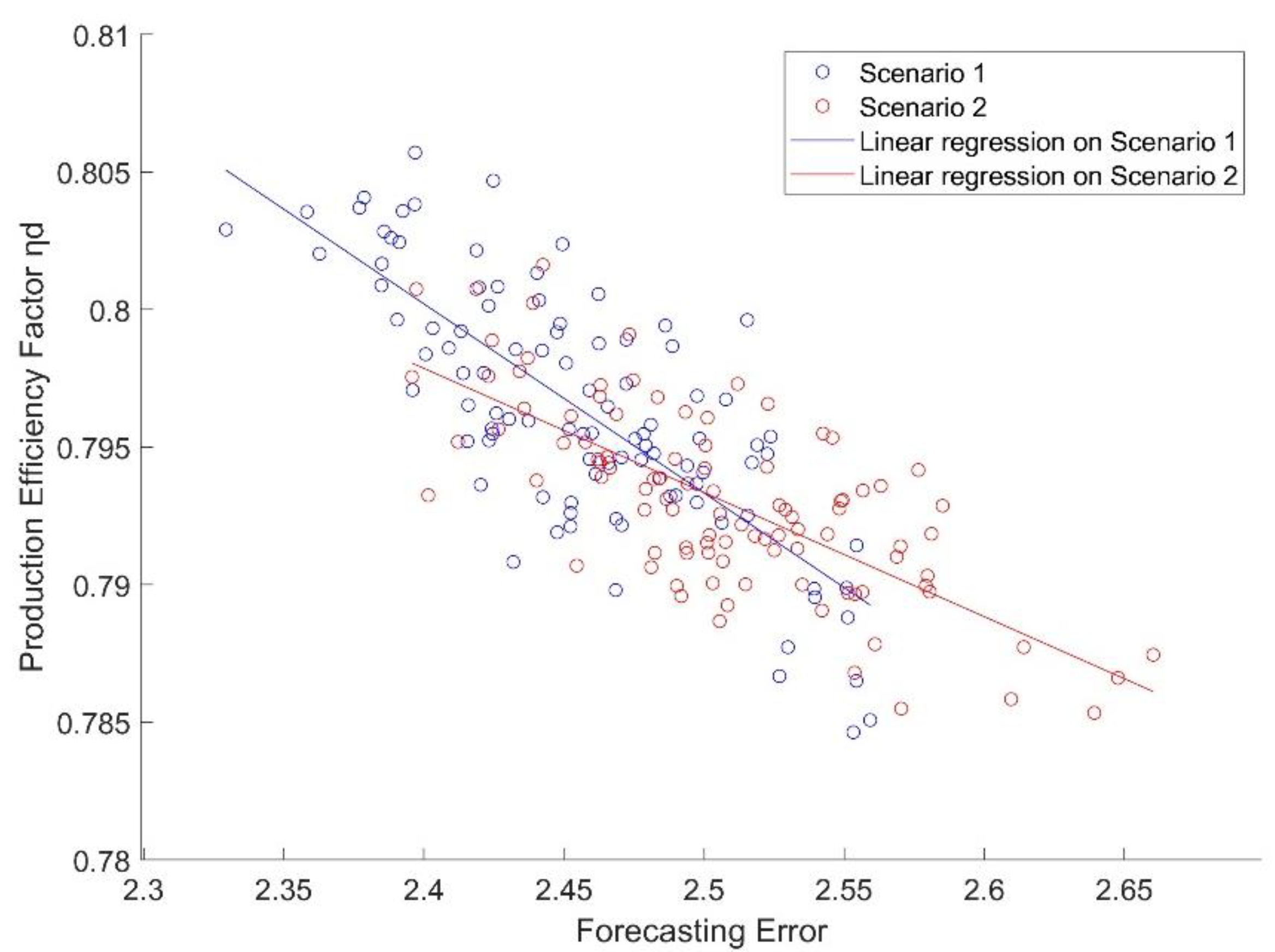
As can be seen in Figure 4, there is a tendency for the production efficiency factor η d to decrease with an increase in the forecast error. The production efficiency factor represents the potential hydropower production in the entire watershed compared to the theoretical maximum production during the same period. η d was found to vary for the hydropower system in the Dalälven River basin, ranging from 78.5% to 80.5% in scenarios 1 and 2, depending on the three month forecast error. This range of variation depends on the forecast error and could appear to be small but can, in principle, represent a substantial economic value for the management of the hydropower production system. For example, if the periodic nature of water runoff in forecasting can be improved by the entire forecasting error range (2.65–2.35 = 0.4) considering the best and the worst possible cases of scenarios 1 and 2, the production efficiency varies by 2%. It can be expected that the yearly energy production of the Dalälven River basin would be enhanced by 80 GWh/year (4 TWh/year × 2% = 80 GWh/year), based on the current production of approximately 4 TWh/year. The reduction in forecasting error from scenario 2 (with forecasts representing a dry year under wet year conditions) to scenario 1 (with forecasts representing a wet year under wet year conditions) corresponds to a production efficiency improvement of about 0.33% (or 13.2 GWh/year), which is obtained by calculating the difference between the mean production efficiency factors of scenarios 1 and 2.
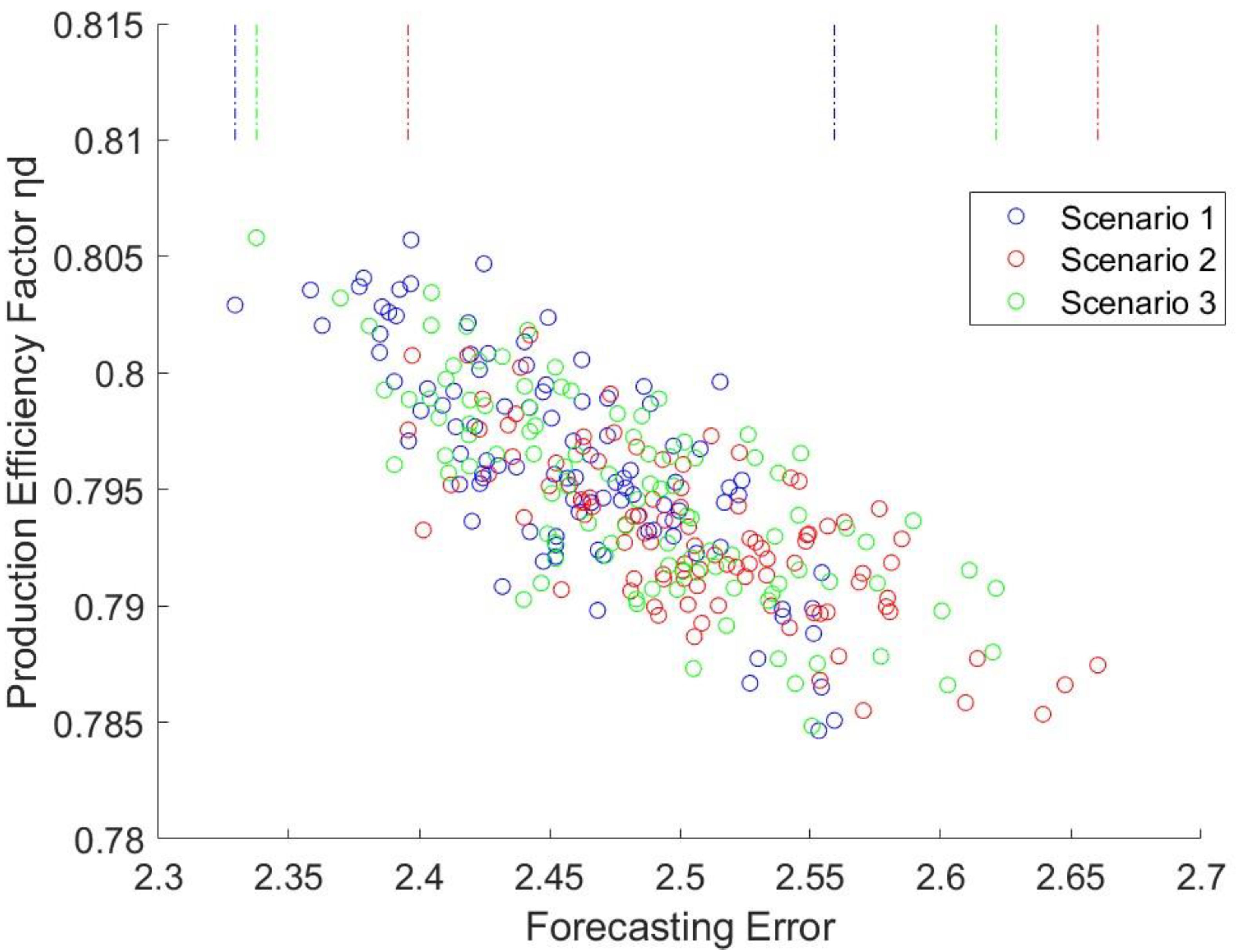
The blue and red lines in Figure 4 present the linear regressions of scenarios 1 and 2 that are bounded by the scenario intervals. The regression lines indicate that scenario 1 has a higher production efficiency and lower forecast error than scenario 2. Production is more efficient for scenario 1 than scenario 2 when the forecasting error is smaller than 2.5, but the opposite prevails when the forecasting error is larger than 2.5. The range of the forecast error is relatively similar in scenario 1, but the ranges of production efficiency factors are larger in scenario 1 than in scenario 2. Figure 5 shows all three scenarios and their forecasting error boundaries. The error range of scenario 3 is obviously larger than those of scenarios 1 and 2, and it roughly matches the non-overlapping parts of scenarios 1 and 2. As a control scenario, scenario 3 does not have any periodic treatment on forecasting, so it can provide a neutral solution that should comprise the solutions from scenarios 1 and 2. Figure 5 shows this.

4.2. Start-Month Impact on the Biennial Periodicity

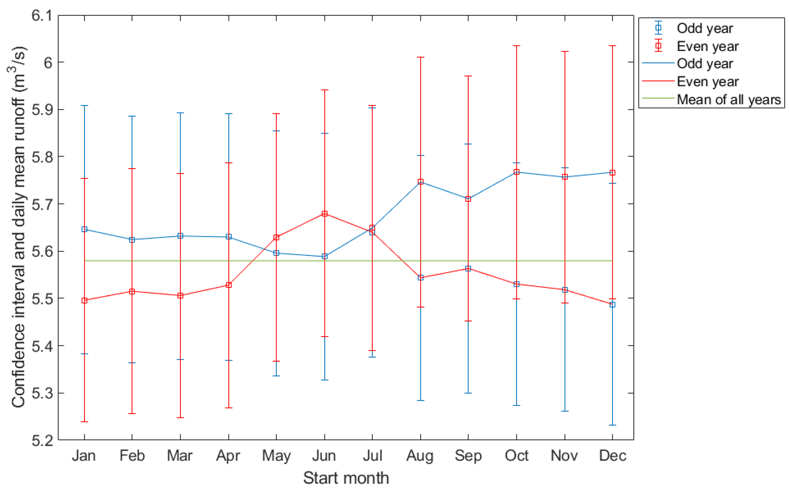
Figure 6 shows the daily mean runoff (m3/s) of 64 subcatchments from the Dalälven River basin. Runoff data were deduced for every set of odd (blue dots) and even (red dots) years using different start months from January to December in the time series that covers daily data from 1961 to 2011. The green line is the average daily runoff of the 64 subcatchments over 51 years. The graph clearly shows that the biennial classification results in differences in the daily mean runoff from the Dalälven River basin, but the pattern depends on the start month of the segments. Note that the odd–even classification used in this figure denotes the year of the start month, but the yearly data selected for a start month later than January cover both odd and even years. The two curves, odd year (blue line) and even year (black line), in Figure 6 highlight an interchange of the implication of odd and even for the dry–wet year characteristic. At the crossing of the curves in Figure 6, both odd and even years are statistically equally wet, whereas the difference becomes larger when the curves are farther apart. The vertical bars show a 95% confidence interval using a t-distribution and indicate somewhat weak significance in the differences between the curves, which can be explained by the prevalence of other periodic climatic phenomena and some degree of randomness. Nevertheless, the results show the systematic biennial hydrological periodicity of the annual mean runoff in the Dalälven River basin, which varies with the start month of the selection and is most vital with a December start month. This circumstance implies that the long-term forecasts used in hydropower production management in December are more sensitive to recognising biennial periodicity compared with planning conducted in a summer month. Compared with the mean runoff of all years (green line), odd years present a higher mean daily runoff than the average, while even years show a relatively low mean daily runoff regardless of the start month.

5. Conclusions and Discussions

This study developed a model framework that assesses the importance of forecasting periodic hydroclimate runoff fluctuations for hydropower planning and generation. Based on 51 years of historical records, the ensemble classification of runoff was shown to possess biennial periodicity, with a strength that was dependent on the start month of the year. This emphasises the importance of focusing on the annual seasonal variation in sub-arctic regions in addition to examining long-term climatic modes of variability. While the model approach is not limited by the selected forecasting method, the historical data sampling representing the complex statistical nature of runoff allows for an evaluation of the effect of periodic errors in runoff forecasts on production efficiency. Forecasting, in combination with the stepwise linear simulation framework, is essential for understanding the implications of periodicity in hydroclimatic variations for the proper operational planning of reservoir storage in cascade hydropower systems. It was found that the forecast errors for the Dalälven River were associated with three month future horizons based on historical data in the range of 3–4% when comparing scenarios 1 and 2, and recognising the biennial periodicity in Dalälven can enhance production efficiency by 1–2%. This may seem small, but it represents substantial economic value in terms of annual production compared to what could be expected from, for example, refurbishing the rock tunnel systems and penstocks of all 36 hydropower stations in the Dalälven River basin, which could also lead to efficiency improvements in the order of a few percent. The main result diagrams (Figure 4) show production efficiency versus forecast errors for two scenarios combining wet year forecasts with wet year scenarios (scenario 1) and dry year forecasts with wet year scenarios (scenario 2). The results indicate that the ensemble classification from which the forecasted runoff is selected plays an important role in enhancing production efficiency. Ignoring the biennial periodicity or the failure to associate future hydrology with a dry or wet year may cause an increase in the forecasting error, thereby decreasing the production efficiency. As a control scenario, scenario 3 verified the results of scenarios 1 and 2 by matching the non-overlapping parts of scenarios 1 and 2 (Figure 5).
The hydropower potential depends on the availability of water in a given stream, and the runoff pattern thus governs the energy generation capacity. This study shows that categorising historical runoff time series from the Dalälven River basin into dry and wet years is statistically possible if the yearly separation is conducted in the appropriate month, generally in mid-winter, but this pattern was found to be much less pronounced when using a mid-summer month. The difference in the annual mean discharge over the 51 year period was in the order of 5% if the separation of wet and dry years started in December. This difference would also be a measure of the possible relative forecast error that can arise in the mean runoff value if the biennial periodicity in water availability as a result of climate fluctuations is neglected.
While this study did not cover techniques for forecasting near-future climatic regimes, it is well known that both GCMs combined with hydrologic downscaling, as well as the statistical assessment of suitable climate indices, are powerful tools to predict current and near-future climate regimes and expected precipitation patterns. Such tools can provide an indication of whether a future year will be dry or wet, but they have lower accuracy when representing short-term fluctuations of importance for the regulatory behaviour in hydropower operations, which is why historical ensemble forecasts can provide essential statistical information in the management process. This assessment model framework can be used to assess the impact of biennial periodicity and can be applied to various periodicities by selecting different periodic ensembles. It could be future research. Some assumptions, like the constant water head and stable reservoir area in the optimisation model, can be improved in future work.
Assessing how biennial hydroclimate fluctuations can be accounted for in the management of hydropower generation and operational planning is essential. The model-based methodology developed in this study can be used to assess the impacts of such fluctuations on hydropower generation and enhance the management of hydropower operations in order to assist the hydropower operator with better planning of water and energy resources.

Author Contributions

Conceptualization, S.H. and A.W.; methodology, S.H. and A.W; software, S.H.; validation, S.H., A.W. and J.R.; formal analysis, S.H. and A.W.; investigation, S.H.; resources, A.W. and J.R.; data curation, S.H.; writing—original draft preparation, S.H.; writing—review and editing, S.H., A.W., J.R. and A.B.-B.; visualization, S.H. and J.R.; project administration, A.W. All authors have read and agreed to the published version of the manuscript.

Funding

This research was funded by the China Scholarship Council, no. 201700260188 and the Swedish Energy Agency (Energimyndigheten), no. 019-005552.

Data Availability Statement

The data, code, and models that support the conclusions of this research are available from the corresponding author upon request.

Acknowledgments

The authors thank the China Scholarship Council and the Swedish Energy Agency (Energimyndigheten) for their financial support. They are also grateful to the Swedish Meteorological and Hydrological Institute and Lund University for collecting the data and providing comments. Moreover, the authors acknowledge the valuable comments of Mikael Amelin. The computations involving high-performance computers were enabled by resources provided by the National Academic Infrastructure for Supercomputing in Sweden (NAISS) and the Swedish National Infrastructure for Computing (SNIC) at https://www.snic.se/ and were partially funded by the Swedish Research Council through grant agreements no. 2022-06725 and no. 2018-05973. We are grateful for these resources.

Conflicts of Interest

The authors declare no conflict of interest.

References

  1. Chang, J.; Wang, X.; Li, Y.; Wang, Y.; Zhang, H. Hydropower plant operation rules optimization response to climate change. Energy 2018, 160, 886–897. [Google Scholar] [CrossRef]
  2. Haguma, D.; Leconte, R.; Côté, P.; Krau, S.; Brissette, F. Optimal Hydropower Generation Under Climate Change Conditions for a Northern Water Resources System. Water Resour. Manag. 2014, 28, 4631–4644. [Google Scholar] [CrossRef]
  3. Tarroja, B.; AghaKouchak, A.; Samuelsen, S. Quantifying climate change impacts on hydropower generation and implications on electric grid greenhouse gas emissions and operation. Energy 2016, 111, 295–305. [Google Scholar] [CrossRef]
  4. de Queiroz, A.R.; Faria, V.A.D.; Lima, L.M.M.; Lima, J.W.M. Hydropower revenues under the threat of climate change in Brazil. Renew. Energy 2019, 133, 873–882. [Google Scholar] [CrossRef]
  5. Anghileri, D.; Botter, M.; Castelletti, A.; Weigt, H.; Burlando, P. A Comparative Assessment of the Impact of Climate Change and Energy Policies on Alpine Hydropower. Water Resour. Res. 2018, 54, 9144–9161. [Google Scholar] [CrossRef]
  6. Forrest, K.; Tarroja, B.; Chiang, F.; AghaKouchak, A.; Samuelsen, S. Assessing climate change impacts on California hydropower generation and ancillary services provision. Clim. Change 2018, 151, 395–412. [Google Scholar] [CrossRef]
  7. van Vliet, M.T.H.; Wiberg, D.; Leduc, S.; Riahi, K. Power-generation system vulnerability and adaptation to changes in climate and water resources. Nat. Clim. Chang. 2016, 6, 375–380. [Google Scholar] [CrossRef]
  8. IPCC. Climate Change 2013—The Physical Science Basis; Cambridge University Press: Cambridge, UK, 2014. [Google Scholar] [CrossRef]
  9. Foster, K. Hydrological Seasonal Forecasting; Lund University: Lund, Sweden, 2019. [Google Scholar]
  10. Uvo, C.B.; Foster, K.; Olsson, J. The spatio-temporal influence of atmospheric teleconnection patterns on hydrology in Sweden. J. Hydrol. Reg. Stud. 2021, 34, 100782. [Google Scholar] [CrossRef]
  11. Wörman, A.; Lindström, G.; Riml, J. The power of runoff. J. Hydrol. 2017, 548, 784–793. [Google Scholar] [CrossRef]
  12. Schmidt, R.; Petrovic, S.; Güntner, A.; Barthelmes, F.; Wünsch, J.; Kusche, J. Periodic components of water storage changes from GRACE and global hydrology models. J. Geophys. Res. Solid Earth 2008, 113, 1–14. [Google Scholar] [CrossRef]
  13. Poveda, G.; Mesa, O.J. Feedbacks between Hydrological Processes in Tropical South America and Large-Scale Ocean–Atmospheric Phenomena. J. Clim. 1997, 10, 2690–2702. [Google Scholar] [CrossRef]
  14. Rajagopalan, B.; Lall, U. Interannual variability in western US precipitation. J. Hydrol. 1998, 210, 51–67. [Google Scholar] [CrossRef]
  15. Krokhin, V.; Luxemburg, W.M.J. Temperatures and precipitation totals over the Russian Far East and Eastern Siberia: Long-term variability and its links to teleconnection indices. Hydrol. Earth Syst. Sci. 2007, 11, 1831–1841. [Google Scholar] [CrossRef]
  16. Lopez, M.G.; Crochemore, L.; Pechlivanidis, I.G. Benchmarking an operational hydrological model for providing seasonal forecasts in Sweden. Hydrol. Earth Syst. Sci. 2021, 25, 1189–1209. [Google Scholar] [CrossRef]
  17. Voisin, N.; Dyreson, A.; Fu, T.; O’Connell, M.; Turner, S.W.; Zhou, T.; Macknick, J. Impact of climate change on water availability and its propagation through the Western U.S. power grid. Appl. Energy 2020, 276, 115467. [Google Scholar] [CrossRef]
  18. Chowdhury, A.F.M.K.; Dang, T.D.; Nguyen, H.T.T.; Koh, R.; Galelli, S. The Greater Mekong’s Climate-Water-Energy Nexus: How ENSO-Triggered Regional Droughts Affect Power Supply and CO2 Emissions. Earth’s Futur. 2021, 9, 1–19. [Google Scholar] [CrossRef]
  19. Siala, K.; Chowdhury, A.K.; Dang, T.D.; Galelli, S. Solar energy and regional coordination as a feasible alternative to large hydropower in Southeast Asia. Nat. Commun. 2021, 12, 4159. [Google Scholar] [CrossRef]
  20. Marco, J.B.; Harboe, R.; Salas, J.D. Stochastic Hydrology and its Use in Water Resources Systems Simulation and Optimization; Springer: Dordrecht, The Netherlands, 1993. [Google Scholar] [CrossRef]
  21. Feiring, B.R.; Sastri, T.; Sim, L.S.M. A stochastic programming model for water resource planning. Math. Comput. Model. 1998, 27, 1–7. [Google Scholar] [CrossRef]
  22. Yevjevich, V. Stochastic models in hydrology. Stoch. Hydrol. Hydraul. 1987, 1, 17–36. [Google Scholar] [CrossRef]
  23. Tiberi-Wadier, A.L.; Goutal, N.; Ricci, S.; Sergent, P.; Taillardat, M.; Bouttier, F.; Monteil, C. Strategies for hydrologic ensemble generation and calibration: On the merits of using model-based predictors. J. Hydrol. 2021, 599, 126233. [Google Scholar] [CrossRef]
  24. Wu, L.; Seo, D.-J.; Demargne, J.; Brown, J.D.; Cong, S.; Schaake, J. Generation of ensemble precipitation forecast from single-valued quantitative precipitation forecast for hydrologic ensemble prediction. J. Hydrol. 2011, 399, 281–298. [Google Scholar] [CrossRef]
  25. Yuan, F.; Berndtsson, R.; Zhang, L.; Uvo, C.B.; Hao, Z.; Wang, X.; Yasuda, H. Hydro Climatic Trend and Periodicity for the Source Region of the Yellow River. J. Hydrol. Eng. 2015, 20, 05015003. [Google Scholar] [CrossRef]
  26. Engström, J.; Uvo, C.B. Effect of Northern Hemisphere Teleconnections on the Hydropower Production in Southern Sweden. J. Water Resour. Plan. Manag. 2016, 142, 5015008. [Google Scholar] [CrossRef]
  27. Hyndman, R.J.; Koehler, A.B. Another look at measures of forecast accuracy. Int. J. Forecast. 2006, 22, 679–688. [Google Scholar] [CrossRef]
  28. Prestwich, S.; Rossi, R.; Tarim, S.A.; Hnich, B. Mean-based error measures for intermittent demand forecasting. Int. J. Prod. Res. 2014, 52, 6782–6791. [Google Scholar] [CrossRef]
  29. Kokko, V.; Hjerthén, P.; Ingfält, H.; Löwen, K.E.; Sjögren, A. Development of Dalälven hydro power scheme in Sweden. Houille Blanche 2015, 6368, 5–14. [Google Scholar] [CrossRef]
  30. Lindström, G.; Pers, C.; Rosberg, J.; Strömqvist, J.; Arheimer, B. Development and testing of the HYPE (Hydrological Predictions for the Environment) water quality model for different spatial scales. Hydrol. Res. 2010, 41, 295–319. [Google Scholar] [CrossRef]
Figure 1. Flowchart of the model framework.
Water 15 01559 g001
Figure 2. The Dalälven River basin with hydropower stations marked with red dots.
Water 15 01559 g002
Figure 3. Ensemble classifications for runoff forecasting in wet years (odd years) and dry years (even years).
Water 15 01559 g003
Figure 4. Comparison of scenario 1 (forecasts of wet years) and scenario 2 (forecasts of dry years), with both scenarios using simulated real runoff from a wet year.
Water 15 01559 g004
Figure 5. Scenarios 1, 2, and 3 and their forecasting error boundaries (dashed lines).
Water 15 01559 g005
Figure 6. Averaged daily runoff (m3/s) over 1961–2011 for the 64 subcatchments of the Dalälven River basin in units of m3/s using different start months. Each start month provides up to 25 yearly samples in odd or even years, and the bars indicate the 95% confidence interval of the mean value estimate (using a t-distribution).
Water 15 01559 g006
Table 1. List of parameters.
ParameterDefinitionParameter Value in the Example Application
T H Time horizon of optimisation: the duration of the forecasted time series placed into one optimisation procedure. T H = 90 (days)
T s i m Period of simulation: the maximum shift in time of the horizon in the receding horizon approach; T s i m = K × t u . T s i m = 90 (days)
t u Updating period: the time during which the decided turbine discharges are applied, whereafter the reservoir levels are updated and new decisions are taken; t u = T s i m / K . t u = 2 (days)
Δ t Numerical time step used to represent the watershed dynamics and to move between the states used in the optimization. Δ t = 0.5 (days)
j j = 1 : J . Index for the numerical time step for water dynamics; J = T H / Δ t . J = 180
i i = 1 : M Index for the reservoirs. M = 49
n n = 1 : N . Index for the repetition number of one updating period simulation with different stochastic runoff forecasts, which was used to make the average decision. N = 10
k k = 1 : K . Index for the simulation time step in order to progress over the simulation period T s i m . The number of updating time steps is K = T s i m / t u . K = 45
Disclaimer/Publisher’s Note: The statements, opinions and data contained in all publications are solely those of the individual author(s) and contributor(s) and not of MDPI and/or the editor(s). MDPI and/or the editor(s) disclaim responsibility for any injury to people or property resulting from any ideas, methods, instructions or products referred to in the content.