Data-Driven Parameter Prediction of Water Pumping Station

Abstract

In the construction process of an intelligent pumping station, the parameter calibration of the pumping station unit is very important. In actual engineering, the working parameters of the pumping station are affected by complex working conditions and natural factors, so that it is difficult to establish a traditional physical model for the pumping station. This paper uses a data-driven method to apply the hybrid model of the convolutional neural network (CNN) and long-term short-term memory network (LSTM) to water level prediction in pumping stations and adds self-attention mechanism feature selection and a bagging optimization algorithm. Then, after an error analysis of the hybrid model, a performance comparison experiment with the separate model was conducted. The historical data of the pumping station project provided by the Tuancheng Lake Management Office of Beijing South-to-North Water Diversion Project was used to train and verify the proposed pumping station water level prediction model. The results show that the CNN–LSTM model based on the self-attention mechanism has higher accuracy than the separate CNN model and LSTM model, with a correlation coefficient (R²) of 0.72 and a mean absolute error (MAE) of 19.14. The model can effectively solve the problem of water level prediction in the front and rear pools under complex pumping station conditions.

1. Introduction

Due to the unbalanced distribution of water resources in time and space, the contradiction between supply and demand of water resources is very prominent in many countries. As one of the 13 water-poor countries in the world, China’s water shortage has posed a serious threat to the sustainable development of society and the economy. As a result, many diversion canals with cascade pumping stations were established in China [1], such as the South-to-North Water Diversion Project. Large-scale water diversion projects have made a major contribution to alleviating the problem of uneven distribution of water resources in the country. As an indispensable and important part of water conservancy projects, pump stations are of great significance to water conservancy construction during their operation. The main task of the pumping station is to undertake the tasks of flood control and waterlogging prevention, water diversion irrigation, and domestic water supply in the area where the pumping station is located. The water level of the pumping station is an important parameter in the operation process. It can judge whether the operation is stable and can provide a warning in case of risk. If the water level between adjacent pumping stations changes sharply, it may cause water supply interruption and severe hydraulic oscillation [2]. In order to build a smart pumping station project based on digital twins, we need to improve the prediction accuracy of the water level parameters of the pumping station.

This research involves nine pumping stations. The rear pool of the front pumping station is connected to the forebay of the rear pumping station. To achieve accurate prediction, it is necessary to consider the startup time of the station, blade angle, voltage, current, and other parameters, including the influence of the forebay water level of the pumping station connected to it. Therefore, it is of great significance to establish a data-driven water level prediction model.

Pumping stations are common regulating facilities in water distribution systems, which have complex hydraulic characteristics and parameters [3]. The method based on physical modeling mainly combines the hydrological model and hydrodynamic model to simulate the whole complex system [4,5,6,7,8,9,10]. Das et al. proposed a novel probabilistic nonlinear method based on a hybrid Bayesian network model with exponential residual correction for daily forecasting of reservoir water levels [11]. Wei et al. used a multilayer perceptron (MLP) to predict hydrological information such as watershed runoff, forebay water level, and pump flow [12]. Liu et al. proposed a hybrid Bayesian vine model for water level information prediction [13]. Lei, X. et al. proposed a pumping station parameter correction method based on data assimilation, established a one-dimensional hydrodynamic model with the inner boundary of the pumping station, and used an integrated Kalman filter to correct the pumping station parameters. The application potential of a support vector machine (SVM) in water level prediction has been explored [14,15]. Tao, H. et al. proposed a hybrid machine learning model based on correlation vector machine and improved Grasshopper optimization for water level prediction [16]. A wavelet neural network (WNN) has also been applied to the water level prediction task [17,18,19,20,21,22].

With the deepening of this research, it is proposed to use artificial intelligence and deep learning technology to monitor and predict the water level of a pumping station. Liu, W.C et al. used the combination of a physics-based model and an artificial neural network-genetic algorithm to improve the prediction accuracy of the hydrodynamic model [23]. Hasan et al. proposed to use artificial intelligence technology to monitor and predict the water level of an underground dam in a double pumping station gold mine, and applied six single classifier methods including support vector machines, artificial neural networks, and naive Bayesian classifiers. Following this premise, a new method based on determining the mutual information of classifiers is proposed [24]. Bazartseren et al. used artificial neural networks (ANNs) and neuro-fuzzy systems for short-term water level prediction [25]. Chang, F.J. et al. used a method based on a recurrent neural network for real-time multistep water level prediction [26].

In the following research tasks, the deep neural network model was applied more frequently to industrial parameter prediction tasks [27,28]. Ren et al. utilized multilayer perceptron (MLP) and a recurrent neural network (RNN) to build a water level prediction model with augmented data containing multiple channels in the spatial dimension and implicit correlations between multiple data records in the temporal dimension [29]. Yuan et al. used a long short-term memory (LSTM) network and a seasonal autoregressive integrated moving average (SARIMA) model to construct a multi-station daily water level prediction model [30]. Han et al. proposed a rainfall-runoff model based on ANN and LSTM for runoff prediction in the Russian River Basin [31]. The CNN–LSTM hybrid model has shown good performance in many prediction tasks [32]. For example, Barzegar et al. built a CNN–LSTM coupled model to predict water quality variables [33]. Yang et al. used the combined model of CNN and LSTM to predict the groundwater level, and the accuracy was better than that of other models [34].

Based on the previous research, this paper proposes a CNN–LSTM pumping station water level prediction model based on the attention mechanism, and considers the different rainfall in the rainy and dry seasons to predict the water level parameters of the pumping station with higher accuracy, replacing the traditional model. The cumbersome mathematical modeling method saves a great amount of labor costs and reduces engineering risks. The contributions of this study are as follows:

(1)

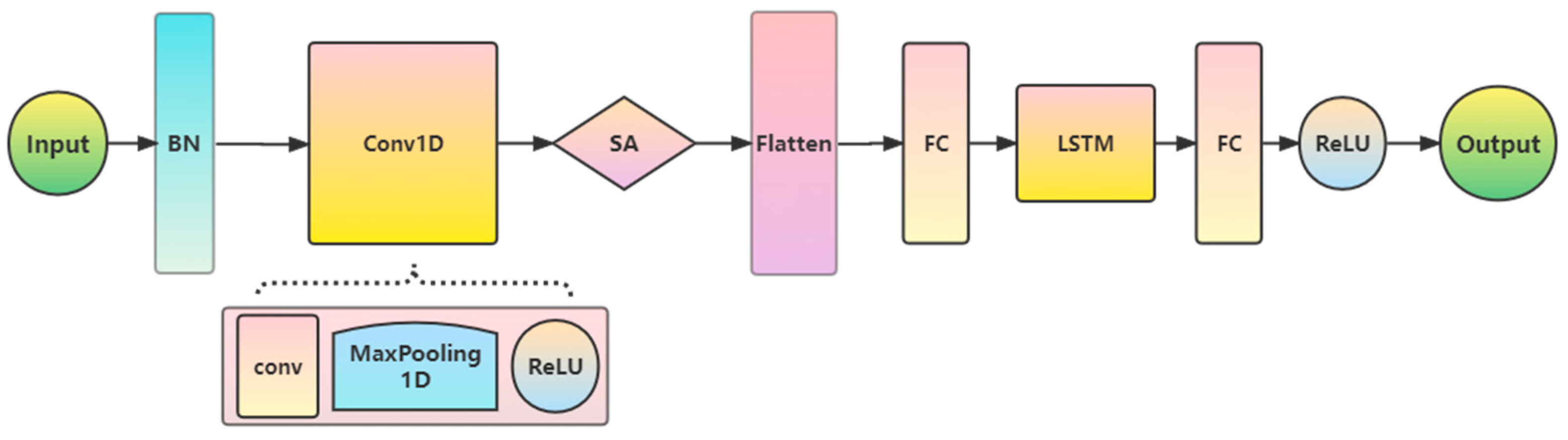
A coupled CNN–LSTM deep neural network model is established for pumping station water level prediction, in which the CNN can extract the relationship between many features of the pumping station and an LSTM can also capture time series information with high prediction accuracy.

(2)

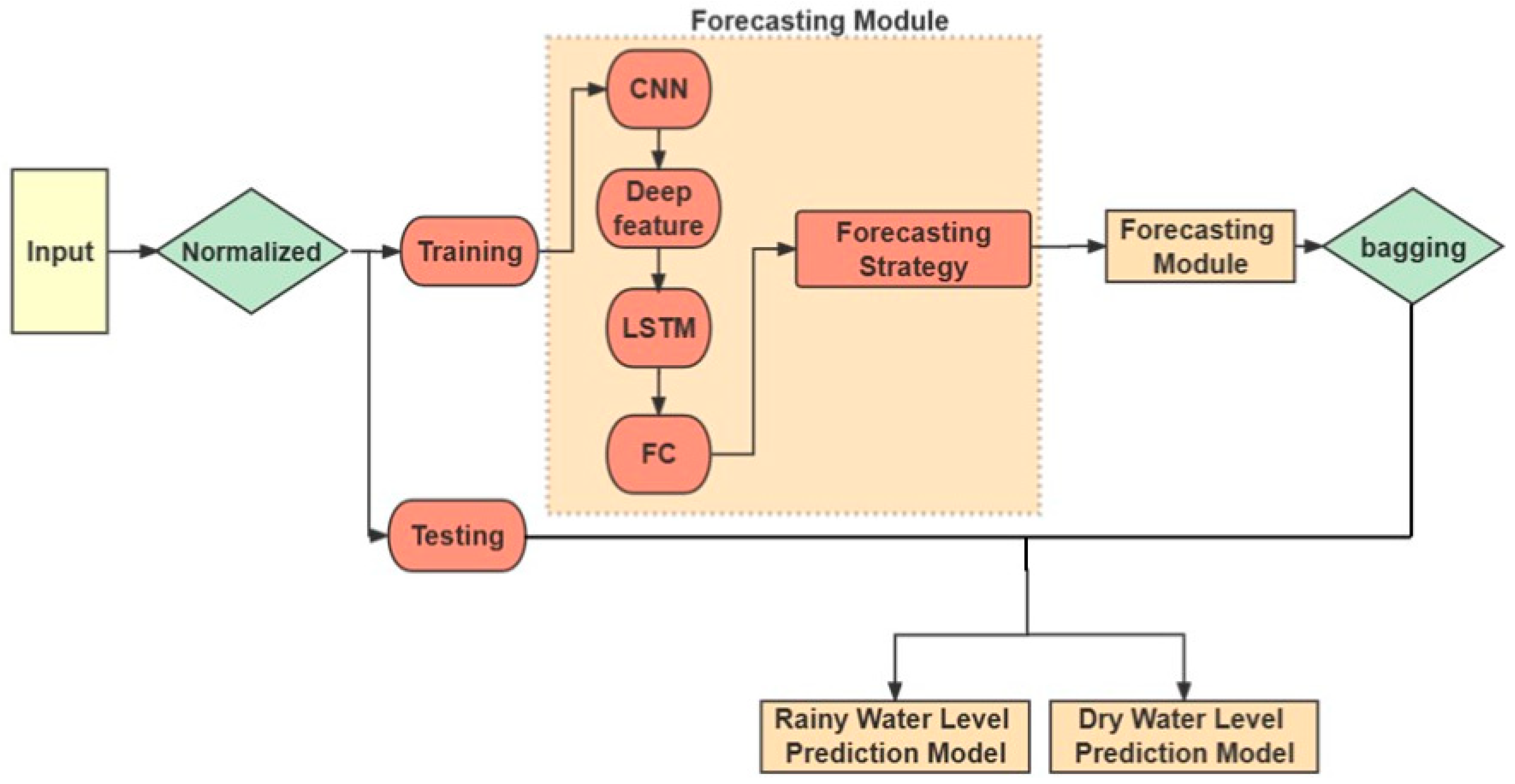
The self-attention mechanism (SA) is used to optimize the CNN, so that the model can better analyze the feature information contained in the vector, and further sort the feature importance. Finally, the bagging method is used to improve the accuracy and stability of the prediction results, making the model more robust.

(3)

Compare the model with the traditional machine learning algorithm support vector regression (SVR), a separate CNN, and a separate LSTM to prove its feasibility and superiority. Although the studies described above explored the ability of these methods to predict water level parameters, no studies compared their performance. Furthermore, to the best of the authors’ knowledge, this is the first time that a coupled CNN–LSTM model has been used to predict water level issues in pumping station projects.

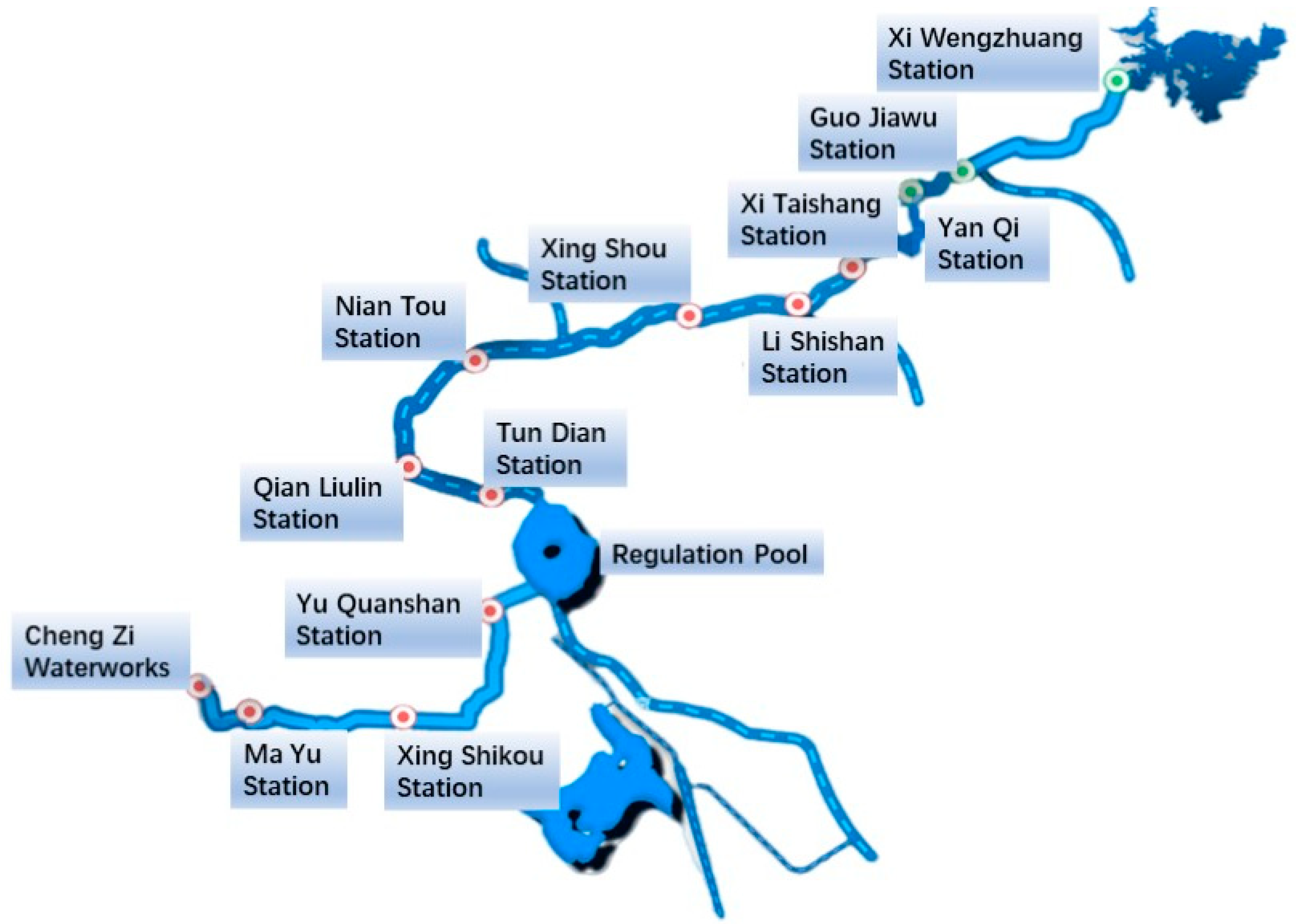
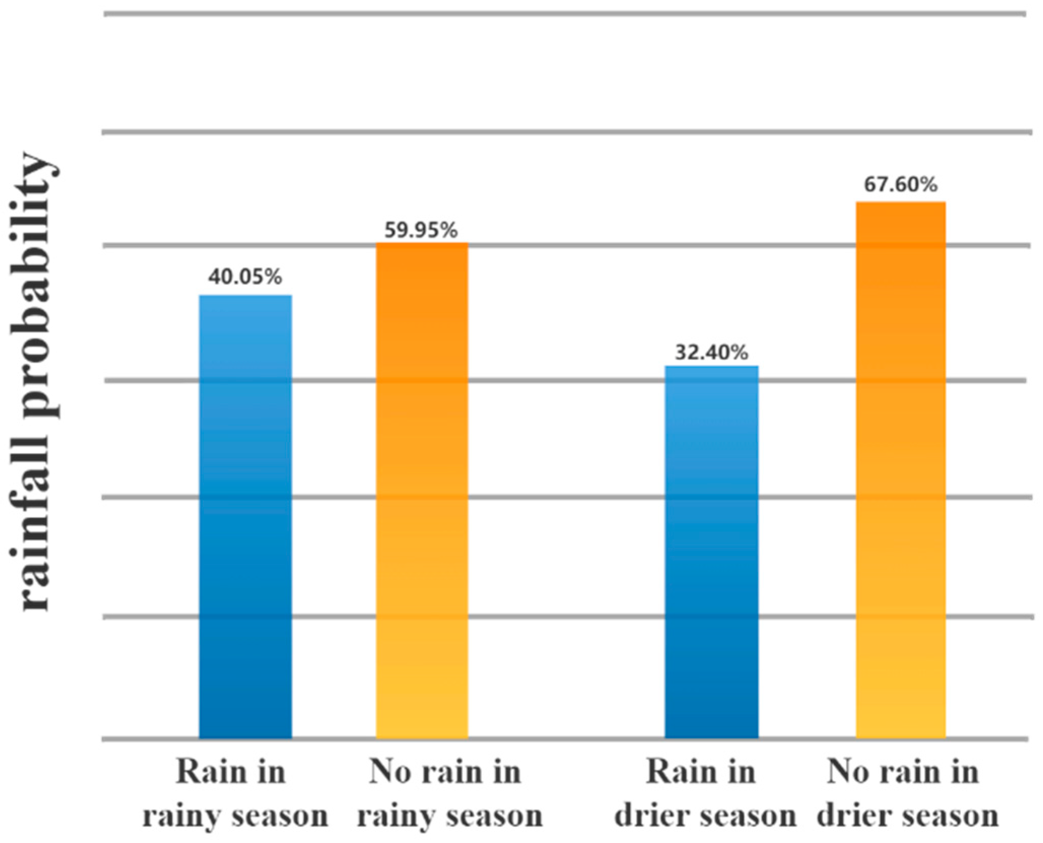
2. Data

The data in this study come from the nine pumping stations in Tundian, Qianliulin, Niantou, Xingshou, Lishishan, Xitaishang, Guojiawu, Yanqi, and Xiwengzhuang involved in the smart pumping station project of the South-to-North Water Diversion Project in Beijing. The database of each station covers the sampling time of the station, startup time, voltage, current, water pump blade angle, pipeline pressure, water pump frequency, running times, current running time, cumulative running time, cumulative flow, reverse cumulative flow, active power, reactive power, vibration and swing of the unit, outlet pressure, pump speed, water level in the inlet pool, and water level in the front and rear pools—a total of 21 dimensions, collected once every minute.

Table 1. Details of the data.

Feature Name	Description	Unit
SAMP_TIME	Samping time	s
START_TIME	Startup time	s
VOLTAGE	Voltage	V
CURRENT	Current	A
IPB_ANGLE	Inlet pump blade angle	°
PIPE_PRESS	Pipeline pressure	Mpa
PUMP_FERQ	Pump frequency	Hz
RUN_NUM	Number Of runs	1
RUN_TIME	This run time	1
CUM_RUN_TIME	Cumulative run time	1
CUM_FLOW	Cumulative flow	m3/s
RE_CUM_FLOW	Reverse cumulative flow	m3/s
ACT_POWER	Active power	kw
REACT_POWER	Reactive power	kw
UNIT_VIB	Unit vibration	μm
UNIT_SWING	Unit swing	mm
OUT_PRESS	Outlet pressure	Mpa
PUMP_SPEED	Pump speed	rpm
INLET_WL	Inlet water level	m
FORE_WL	Fore pool water level	m
REAR_WL	Rear pool water level	m

details the structure of the experimental data.

Figure 1 is the distribution map of the nine stations involved in this paper, depicting the geographical relationship of the nine pumping stations.

Because in northern China, especially in the Beijing-Tianjin-Hebei region, the warm temperate continental climate is very pronounced, the climate with more rain in summer and less rain in winter can easily affect our prediction of the water level of the pumping station. Figure 2, below, is the rainfall distribution map. If we directly use all the data for modeling, the model will not be able to learn the regular characteristics of the data well. Therefore, we divide the data sets according to the seasonal differences, and respectively establish the water level prediction model of the pumping station based on the rainy season and the water level prediction model of the pumping station based on the non-rainy season.

We selected the data from July, August, and September 2020 as the rainy season training set, and the data from November, December, and January 2020 as the non-rainy season training set; we selected August and December 2021 as the test set.

3. Methodology

3.1. Forecasting Strategy

In the forecasting task of time series data, the choice of forecasting strategy plays an important role in the speed and accuracy of forecasting results. There are currently three mainstream forecasting methods: direct multistep forecasting, recursive multistep forecasting, and direct + recursive mixed forecasting strategies. Among them, the essence of direct multistep forecasting is single-step forecasting, and multistep forecasting is formed through the combination of multiple single-step forecasting models. For example, if we want to predict the value of the sequence at three time points, we will build three models: model1, model2 and model3. The problem with this approach is that if we predict N time steps, we need to build N models. The model complexity will become very high, and there will be high variance, especially if we want to predict the time step in a relatively long case; for example, if we want to predict 100 time steps in the future, the nearest known observation sample used in the 100th time step is 100 time steps ago. We know that the closer the period is to the current time point, the better the predictive effect of the lag feature, and the longer the interval, the worse the effect. The essence of recursive multistep forecasting is simple single-step forecasting, but unlike the first case, recursive multistep forecasting does not need to build N models when predicting N time steps, only one model is enough. For example, if we have a three-order lag model: [lag(t − 2), lag(t − 1), lag(t)], and we would like to predict the next three time steps, X, Y, Z, we can use lag(t − 2), lag(t − 1) and lag(t) to predict X, and use the predicted value of X as a feature to obtain [lag(t − 1), lag(t), X], and then use this model to predict Y, and so on. The disadvantage of this method is that the predicted value is used instead of the real data, so the recursive multistep forecasting strategy will accumulate forecasting errors; that is, the deviation of the recursive strategy is large, so as the forecast time range increases, the performance and accuracy of the model will decline rapidly. The direct + recursive hybrid strategy combines the direct strategy and the recursive strategy. The hybrid strategy is to build N models based on N time steps to be predicted, use model1 to predict X to obtain prediction(X), and then use this prediction(X) as the “observation” data of model2, included in the model training.

This paper uses a partially unknown recursive prediction strategy, using the last time window of the training set to predict the first label of the test set, and then adding the predicted label back to the training set. The flow chart of the overall prediction model of this study is shown in Figure 3.

We assume the input sample matrix $X={\left(X_1{X}_2{X}_3\cdots X_n\cdots X_m\right)}^T$, where $X_1-X_n$ is the training set sample and $X_{n+1}-X_m$ is the testing set sample. The label is $Y={\left(y_1{y}_2{y}_3\cdots y_n\cdots y_m\right)}^T$. Each sample can be written as $X_m={\left(X_{m1}{X}_{m2}{X}_{m3}\cdots X_{mj}\right)}^T$, where j is the number of features.

In the training process, assuming t is the sample time step, the model can be regarded as a function f(), and the predicted value can be obtained as shown in Equations (1)–(3):

$$y_{t+1}^O=f\left(X_1,X_2,\cdots X_t;y_1,y_2,\cdots y_t\right)$$

(1)

$$y_{t+2}^O=f\left(X_2,\cdots X_t,X_{t+1};y_2,\cdots y_t,y_{t+1}\right)$$

(2)

$$y_{n+1}^O=f\left(X_{n+1-t},X_{n+2-t},\cdots ,X_n;y_{n+1-t},y_{n+2-t},\cdots ,y_n\right)$$

(3)

During testing, we used $y_{n+1}^O$ to infer $X_{n+1}^O$, added $X_{n+1}^O$ back to the training set, predicted $y_{n+2}^O$, continued to infer $X_{n+2}^O$, then added this back to the training set, predicted $y_{n+3}^O$, and so on. The specific implementation process is shown in Equations (4)–(6):

$$y_{n+2}^O=f\left(X_{n+2-t},\cdots ,X_n,X_{n+1}^O;y_{n+2-t},\cdots ,y_n,y_{n+1}^O\right)$$

(4)

$$y_{n+3}^O=f\left(X_{n+3-t},\cdots ,X_n,X_{n+1}^O,X_{n+2}^O;y_{n+3-t},\cdots ,y_n,y_{n+1}^O,y_{n+2}^O\right)$$

(5)

$$y_{n+4}^O=f\left(X_{n+4-t},\cdots ,X_n,X_{n+1}^O,X_{n+2}^O,X_{n+3}^O;y_{n+4-t},\cdots ,y_n,y_{n+1}^O,y_{n+2}^O,y_{n+3}^O\right)$$

(6)

The predictive strategies for training and testing are shown in Figure 4 and Figure 5 below.

3.2. Convolutional Neural Network (CNN)

A convolutional neural network (CNN) is a feedforward neural network [35]. It is one of the representative algorithms of deep learning [36,37,38]. Each neuron only affects a part of the neurons in the adjacent layer and has a local receptive field. Therefore, the convolutional neural network has a strong ability to capture local features [39]; on the other hand, through weight sharing and pooling, the computational complexity of the network is significantly reduced, making the CNN widely used [40]. A CNN is an outstanding algorithm in the field of image classification and speech recognition. It is also the core technology of most computer vision systems, from Facebook’s automatic image labeling to self-driving cars, and even of AlphaGo. At the same time, a CNN has gradually been applied to NLP tasks in the past two years. In sentence classification, the CNN-based model has achieved very significant results. Convolution operation is the most significant feature that distinguishes it from other neural network models. The classic convolutional neural network mainly includes the following five layers: input layer, output layer, convolution layer, pooling layer, and fully connected layer. Among them, the convolutional layer continuously extracts features, from local features to overall features. The pooling layer extracts the main features of a certain area, reduces the number of parameters, and prevents the model from overfitting. The fully connected layer is equivalent to the feature space transformation, which realizes the extraction and integration of useful information.

For sequence data, we use a one-dimensional convolutional network structure for text processing.

After the convolution operation, an activation function needs to be passed. The role of the activation function is to add nonlinear factors, because the expressive power of the linear model is not enough. This study uses the rectified linear activation unit (ReLU) function as the activation function, as shown in Formulas (7) and (8):

$$ReLU\left(x\right)=\left\{\begin{array}{c}x\hspace{1em}if\left(x\right)>0\\ 0\hspace{1em}if\left(x\right)\le 0\end{array}\right.$$

(7)

$$y_j^l=ReLU\left({\displaystyle \sum }_{i\in M_j}{X}_j^{l-1}\ast k_{ij}^l+b_j^l\right)$$

(8)

Among them, $y_j^l$ is referred to as the output of the jth channel of the convolutional layer l, which is obtained by performing convolution summation and offset on the output feature map $X_j^{l-1}$ of the previous layer, and then passes through the ReLU activation function. $k_{ij}^l$ is the convolution kernel matrix, and $b_j^l$ is the bias to the features after convolution. For an output feature map $X_j^l$, the convolution kernel $k_{ij}^l$ corresponding to each input feature map $X_j^{l-1}$ may be different; “∗” is the convolution symbol and its relevant definitions are shown in Formula (9); a one-dimensional CNN is used in this study.

$$z\left(t\right)=x\left(t\right)\ast y\left(t\right)=\int x\left(m\right)y\left(t-m\right)dm$$

(9)

The pooling layer is sandwiched between consecutive convolutional layers to compress the amount of data and parameters and reduce overfitting. There are three types of pooling layers: average pooling, maximum pooling, and random pooling. Our study uses max pooling.

After a series of convolutions, activations, and pooling, the one-dimensional convolutional neural network generates feature vectors and inputs them into the LSTM network. The output is shown in (10):

$$Y=ReLU{\displaystyle (}ReLU{\displaystyle (}\cdots ReLU{\displaystyle (}{\displaystyle \sum }_{i\in M_j}{X}_j^{l-1}\ast k_{ij}^l+b_j^l{\displaystyle )}{\displaystyle )}{\displaystyle )}$$

(10)

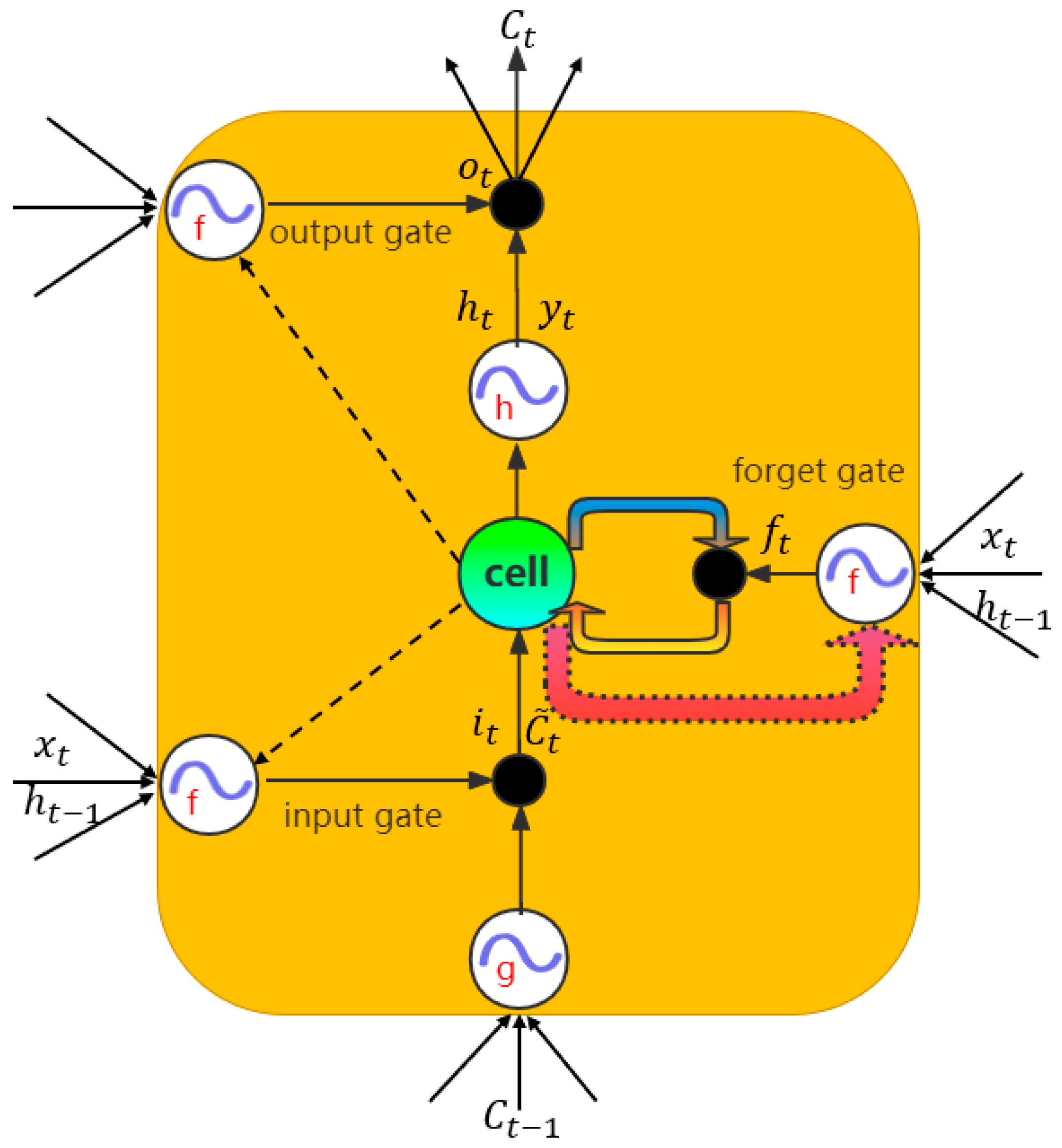
3.3. Long Short-Term Memory (LSTM)

The full name of LSTM is long short-term memory. It was proposed by Hochreiter and Schmidhuber (1997), improved and promoted by Alex Graves [41], and is now widely used in the field of machine learning. The LSTM model is a variant deep learning model based on a recurrent neural network (RNN), which can solve the problems of gradient disappearance and short-term memory in the RNN model, and capture long-term dependencies [42]. Compared with ordinary RNN, the most critical improvement of LSTM is the addition of cell state and gate structure, which retains the characteristics of a long time ago through the control of the gate. The LSTM model is an effective and scalable model for solving learning problems related to various time series data. It has been applied in various fields through the combination with other neural networks and speech recognition, language modeling, and translation.

Each cell of LSTM has three parts: forgetting gate, input gate, and output gate, which are respectively responsible for information flow screening, memory, and generation.

The information part that needs to be filtered out in each decomposed signal component is determined through the forgetting gate. The current input and the state of the previous moment are used to determine whether to filter through the sigmoid function:

$$f_t=\sigma \left(W_f·\left[h_{t-1},x_t\right]+b_f\right)$$

(11)

The input information is determined by the sigmoid function to retain the part. Parts $x_t$ and $h_{t-1}$ become the new ${\tilde{C}}_t$ value after being updated by tanh. Then, $C_{t-1}$ is updated to $C_t$. The specific process is shown in Equations (12)–(14):

$$i_t=\sigma \left(W_i·\left[h_{t-1},x_t\right]+b_i\right)$$

(12)

$${\tilde{C}}_t=\mathit{tanh}\left(W_c·\left[h_{t-1},x_t\right]\right)+b_C)$$

(13)

$$C_t=f_t{C}_{t-1}+i_t{\tilde{C}}_t$$

(14)

First, the unit output part is determined by the sigmoid function, and then the unit state is multiplied by the output part of the tanh and the sigmoid gate to obtain the predicted value point of the model, as shown in Formulas (15) and (16):

$$o_t=\sigma \left(W_o·\left[h_{t-1},x_t\right]+b_o\right)$$

(15)

$$h_t=o_t\mathit{tanh}\left(C_t\right)$$

(16)

Figure 6, below, describes the workflow of LSTM.

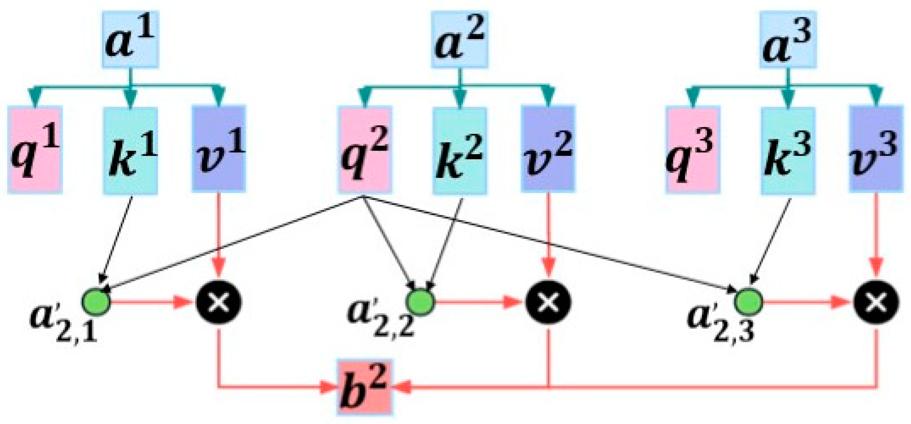
3.4. Self-Attention Mechanism

Attention is a unique cognitive ability of human beings, which means that people can selectively ignore some nonimportant information while paying attention to certain information. The attention mechanism (attention) model screens out a small amount of important information from a large amount of information, and focuses on this important information, ignoring most of the unimportant information. This basis allows the neural network to observe where it needs to pay attention at different time nodes, thereby improving the accuracy of the model. Self-attention is a variant of the attention mechanism, which uses the inherent information of the data features to interact with attention as much as possible. Its basic structure is shown in Figure 7.

For self-attention, the same input is mapped to different spaces to obtain three matrices, $Q$, $K$, and $V$, composed of query vector query, key vector key, and value vector value, respectively. First, we calculated the dot product between $Q$ and $K$, divided by a scale $\sqrt{D_k}$, where $D_k$ is the dimension between the query vector and the key vector, obtained the correlation weight matrix coefficient of $Q$ and $K$, and then used the softmax function to obtain the correlation. The weight matrix coefficients were normalized, and, finally, multiplied by the matrix $Q$ to obtain the vector sequence representation of self-attention in the current node. The calculation formula for this operation is shown in Formula (17):

$$A_{attention}\left(Q,K,V\right)=V_{softmax}\left(\frac{Q{K}^T}{\sqrt{D_k}}\right)$$

(17)

$Q$, $K$, $V$ are matrices composed of vectors obtained by the same input through different linear transformations and $\sqrt{D_k}$ is a scaling factor to keep the gradient stable during training. After calculating the attention score function, $softmax\left(·\right)$ is the activation function normalized by the column for normalization. This process can be explained by Formula (18):

$$\begin{array}{l}{a}_{t,i}=softmax\left(s_{t,i}\left(x_t,h_{t-1},q_t\right)\right)\\ =\frac{\exp \left(s_{t,i}\left(x_t,h_{t-1},q_t\right)\right)}{{{\displaystyle \sum }}_{j=1}^{\left(1+m\right)\times n}\exp \left(s_{t,j}\left(x_t,h_{t-1},q_t\right)\right)}\end{array}$$

(18)

The self-attention mechanism introduced in this study is mainly used to combine with the CNN, where $a_{t,i}$ is the attention distribution that measures the importance of the i-th dimension of incoming information at time t. At this time, the incoming information coefficient of a single self-attention CNN–LSTM unit is $1+at$. After the CNN initially extracts feature values that have a greater impact on label values, these feature values are further sorted by feature importance. On the one hand, it can reduce the dimensionality, obtain the importance of different sequence data on the water level of the pumping station, and eliminate factors that have little influence on the predicted value; on the other hand, it can reduce the amount of input data to the LSTM network and reduce the computational pressure of training.

3.5. CNN–LSTM Principle Based on Self-Attention Mechanism

The CNN–LSTM model consists of two parts. The first part is a one-dimensional convolutional neural network model based on the self-attention mechanism, and the second part is the long-term short-term memory network LSTM.

Among them, in the first part, the normalized input matrix is passed into the CNN network structure, and then, through the convolutional layer, the one-dimensional pooling layer, and the ReLU activation layer, the feature extraction of the incoming multidimensional time series data is performed. Then, the feature importance is further sorted through the self-attention mechanism. Since the time series data after using CNN for feature extraction still has time series characteristics, the feature matrix output by SA-Conv1D is passed into the LSTM model, through the LSTM layer and the fully connected layer, in turn, and, finally, the prediction result is passed through the ReLU activation function output.

Figure 8, below, is the operating structure diagram of the CNN–LSTM model.

3.6. Bagging Strategy

The integrated learning algorithm itself is not a separate machine learning algorithm, but by constructing and combining multiple machine learners to complete the learning task, it can obtain superior performance to that of a single learner. Currently, there are two common integrated learning algorithms: bagging-based algorithms and boosting-based algorithms. Bagging-based representative algorithms include random forests, and boosting-based representative algorithms include Adaboost, GBDT, XGBoost, etc. This article uses the bagging algorithm.

The idea of bagging is to train k independent base learners and combine the results of each base learner (weighted or majority vote) to obtain a strong learner.

Suppose we have a training set X. After N rounds of uniform probability self-sampling, N self-sampling sample sets $X_1,X_2,X_3,\cdots ,X_N$ are obtained, and the size of each sampling sample set is the same as the number of training sets. Now, for each self-sampled sample set, we have to train a classifier $a_i\left(x\right)$ dedicated to it. The final classifier is the output of the average of all these individual classifiers. In classification algorithms, this process is named voting, as shown in Formula (19):

$$a\left(x\right)=\frac{1}{M}{{\displaystyle \sum }}_{i=1}^M{a}_i\left(x\right)$$

(19)

Figure 9, below, shows the algorithm flow.

Assume that each basic algorithm is $b_1\left(x\right)$, $b_2\left(x\right)$,…, $b_n\left(x\right)$; assuming that there is a real answer $y\left(x\right)$ defined for all inputs, which is the objective function, and the distribution of the data is $p\left(x\right)$, the error of each regression function can be expressed as Formula (20):

$${\epsilon }_i\left(x\right)=b_i\left(x\right)-y\left(x\right),i=1,\cdots ,n$$

(20)

and the expected value of the mean squared error is Formula (21):

$$E_x\left[{\left(b_i\left(x\right)-y\left(x\right)\right)}^2\right]=E_x\left[{\epsilon }_i^2\left(x\right)\right]$$

(21)

Then, the average error of all regression functions is as shown in Formula (22):

$$E_1=\frac{1}{n}{E}_x\left[\sum {\epsilon }_i^2\left(x\right)\right]$$

(22)

We assume that the errors are unbiased and uncorrelated, as shown in Formulas (23) and (24):

$$E_x\left[{\epsilon }_i\left(x\right)\right]=0$$

(23)

$$E_x\left[{\epsilon }_i\left(x\right){\epsilon }_j\left(x\right)\right]=0,i\ne j$$

(24)

Now, let us build a new regression function, as shown in Formula (25), that will average the values of each function:

$$a\left(x\right)=\frac{1}{n}{{\displaystyle \sum }}_{i=1}^n{b}_i\left(x\right)$$

(25)

Its mean square error is:

$$\begin{array}{l}{E}_n=E_x{\left[\frac{1}{n}{\displaystyle {\displaystyle \sum }_{i=1}^n}{b}_i\left(x\right)-y\left(x\right)\right]}^2\\ =E_x{\left[\frac{1}{n}{{\displaystyle \sum }}_{i=1}^n{\epsilon }_i\right]}^2\\ =\frac{1}{n^2}{E}_x\left[{{\displaystyle \sum }}_{i=1}^n{\epsilon }_i^2\left(x\right)+{\displaystyle {\displaystyle \sum }_{i\ne j}}{\epsilon }_i\left(x\right){\epsilon }_j\left(x\right)\right]\\ =\frac{1}{n}{E}_1\end{array}$$

(26)

Therefore, by averaging the individual output answers, we reduce the mean squared error by a factor of n.

Combining the CNN–LSTM network based on the attention mechanism in this study with the bagging ensemble algorithm, the accuracy and robustness of the model are improved after the model has been trained many times.

4. Model Evaluations

To evaluate the performance metrics of the models, we used mean absolute error ($MAE$) and coefficient of determination ($R^2$) to evaluate the predictive power of the model proposed in this study. The formula for the above indicators is shown in Formulas (27) and (28):

$$MAE=\frac{1}{n}{\displaystyle \sum }_{i=1}^n\left|\widetilde{y_i}-y_i\right|$$

(27)

$$\begin{array}{c}{R}^2=1-\frac{{{\displaystyle \sum }}_i{\left(\widehat{y_i}-y_i\right)}^2}{{{\displaystyle \sum }}_i{\left(\overline{y_i}-y_i\right)}^2}\end{array}$$

(28)

In the above formulas, $n$ is the total number of data, $y_i$ is the predicted value, and $\widetilde{y_i}$ is the real value. MAE is the average value of the absolute error, which can reflect the actual situation of the error of the predicted value. The smaller the value, the higher the model accuracy. $R^2$ is the coefficient of determination, which can judge the quality of the model, and its value range is [0, 1]. Generally speaking, the larger the $R^2$, the better the model fitting effect.

5. Results

5.1. Hyperparameter Configuration

Two important factors to achieve good prediction results are efficient training strategy and configuration of hyperparameters. Appropriate hyperparameter configuration can enable the model to learn the deep features of the data and can make the model converge faster and more accurately to achieve the best prediction effect.

In order to intuitively reflect the performance of the CNN–LSTM prediction model based on the attention mechanism, the experiment compared SVR, CNN, LSTM, and CNN–LSTM. In order to ensure fairness in the comparison, the depth and parameter settings of the neural network should be as similar as possible. The list of hyperparameters is shown in

Table 2. The hyperparameter settings.

Model	Parameter	Details	Value
CNN, LSTM, CNN-LSTM	Minibatch	Batch size	128
		Epoch	1000
	L2 regularization	Penalty parameters	0.01
	Decayed learning rate	Initial learning rate	0.01
		Decay rate	0.9
		Decay steps	15
		Minimum learning rate	1.00 × 10−4
	Dropout	Dropout rate	0.001
SVR	Grid search	Kernel function	RBF
		C	1
		Gamma	0.1
	Cross-validation	k-fold	5

below. The self-attention mechanism is also used in the two neural network models of CNN and LSTM.

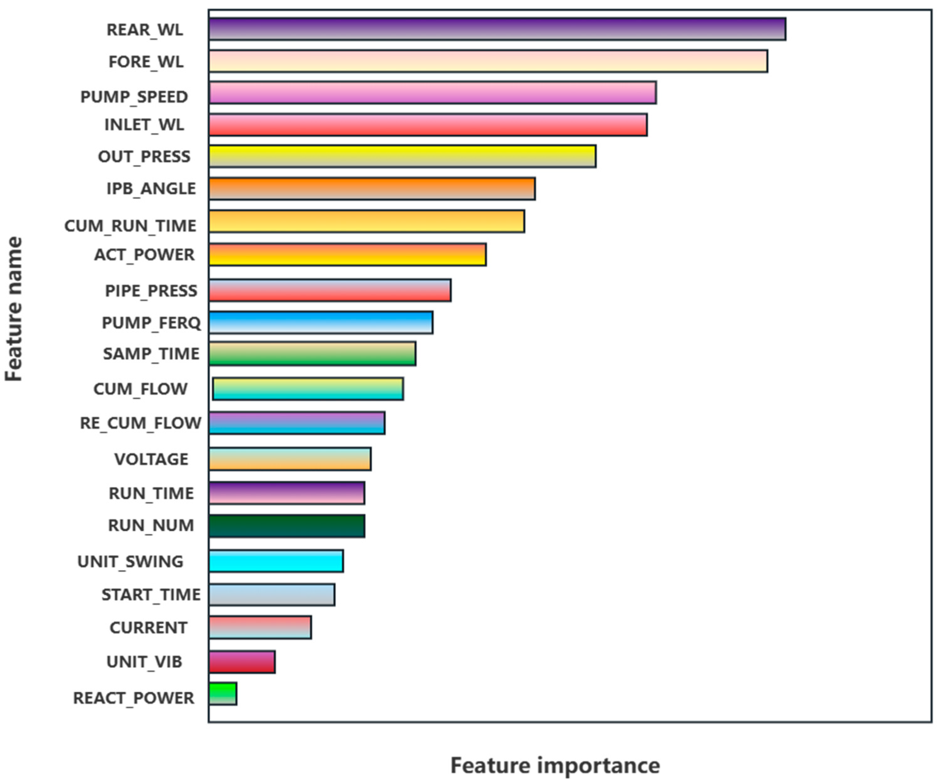
5.2. Feature Selection Results

As shown in Figure 10 below, the water level of the pumping station is determined by many factors, and how to better select features will become an important factor affecting the performance of the model. After the feature selection of the CNN and self-attention mechanism, this model obtained a schematic diagram of the relative importance of each feature and the water level of the pumping station.

The figure above shows the global importance of each feature, where inlet pump blade angle, outlet pressure, pump speed, inlet water level, fore pool water level, and rear pool water level account for 50% of the features’ importance.

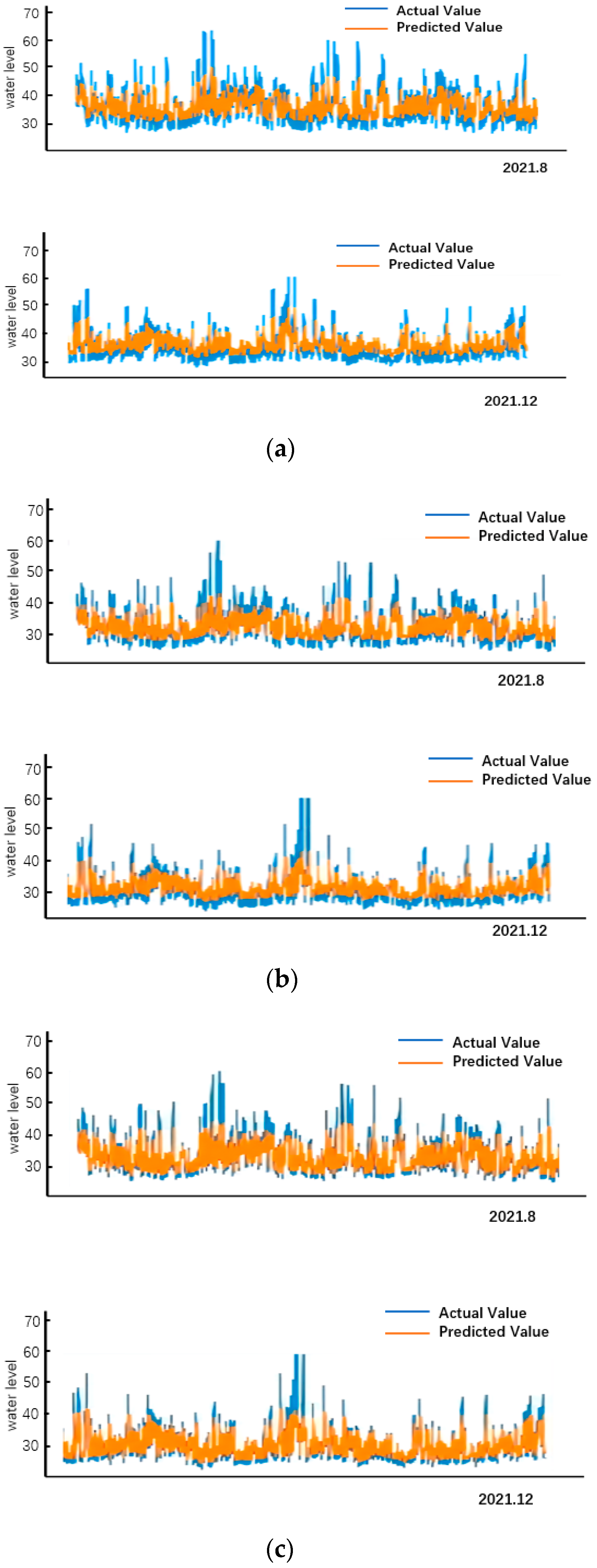
5.3. Comparison of Model Prediction Results

We used SVR, a separate CNN, a separate LSTM, and a CNN–LSTM network to predict the water level of the pool behind the pumping station in August and December 2021, respectively. The comparison between the predicted results and the actual values is shown in Figure 11 below.

6. Discussion

The results show that the one-dimensional CNN–LSTM model based on the self-attention mechanism is very effective in predicting the water level of the pumping station.

From the comparison chart of the predicted value and the actual value of the water level of the pumping station in August 2021 using the rainy season prediction model, it can be seen that the rainy season prediction model has a higher degree of fit than the other three models, and SVR, CNN, and LSTM have a lower water level. The fit is good, but the fit to the water level peak is poor. In contrast, the CNN–LSTM model has a better fit in the face of extreme weather. From the comparison chart of the predicted value and the actual value of the water level of the pumping station in December 2021 using the non-rainy season prediction model, it can be seen that the prediction effect of the non-rainy season water level prediction model and the other three models is not relevant in the case of low water level or peak water level. The fit is better.

From the specific error analysis in

Table 3. Evaluation index.

	Machine Learning Model	Neural Network Model
Indicator	SVR	CNN	LSTM	CNN-LSTM
MAE	31.02	29.37	25.67	19.14
R2	0.30	0.34	0.45	0.72

below, it can be seen that among the four models, the CNN–LSTM model has the smallest MAE value and the largest R². The CNN–LSTM model based on the self-attention mechanism performs relatively well in traditional time series prediction tasks. Compared with the separate LSTM network model, the MAE of the CNN–LSTM network was reduced by 6.53%, and the R² was increased by 0.27%. Although the effect of the rainy season water level prediction model still has advantages over the effects of separate CNN and LSTM models, these are not particularly significant. A large part of the reason for this is the extreme rainfall that has occurred frequently in northern China in recent years, resulting in large fluctuations in water levels. Next, the model will be improved by increasing the amount of data.

7. Conclusions

This study developed a CNN–LSTM model based on the self-attention mechanism for the predicting the water level of a pumping station and used a partially unknown recursive prediction strategy to speed up the training efficiency of the model and improve the model accuracy. TA CNN based on the self-attention mechanism was used to extract short-term gap features and rank the feature importance; then, the hidden features extracted by the CNN were input into LSTM according to different weights for long-term prediction. Finally, using the idea of bagging integration algorithm, the training results of different base learners were combined to form a pumping station water level prediction model for the rainy season and non-rainy season of the pumping station.

There are many areas for improvement in the model. Although the CNN–LSTM model demonstrated better performance than a separate CNN and a separate LSTM model, it also has a certain time lag. It is also necessary to improve the robustness of the model in the face of extreme cases.

References

1. Lu, L.B.; Tian, Y.; Lei, X.H.; Wang, H.; Qin, T.; Zhang, Z. Numerical analysis of the hydraulic transient process of the water delivery system of cascade pump stations. Water Sci. Technol. 2018, 18, 1635–1649. [Google Scholar] [CrossRef]
2. Xu, W.; Chen, C. Optimization of Operation Strategies for an Interbasin Water Diversion System Using an Aggregation Model and Improved NSGA-II Algorithm. J. Irrig. Drain. Eng. 2020, 146, 04020006. [Google Scholar] [CrossRef]
3. Lei, X.; Tian, Y.; Zhang, Z.; Wang, L.; Xiang, X.; Wang, H. Correction of pumping station parameters in a one-dimensional hydrodynamic model using the Ensemble Kalman filter. J. Hydrol. 2019, 568, 108–118. [Google Scholar] [CrossRef]
4. Munar, A.M.C.J. Coupling large-scale hydrological and hydrodynamic modeling: Toward a better comprehension of watershed-shallow lake processes. J. Hydrol. 2018, 564, 424–441. [Google Scholar] [CrossRef]
5. Siddique-E-Akbor, A.H.M.; Hossain, F.; Lee, H.; Shum, C.K. Inter-comparison study of water level estimates derived from hydrodynamic–hydrologic model and satellite altimetry for a complex deltaic environment. Remote Sens. Environ. 2011, 115, 1522–1531. [Google Scholar] [CrossRef]
6. Timbadiya, P.V.; Krishnamraju, K.M. A 2D hydrodynamic model for river flood prediction in a coastal floodplain. Nat. Hazards 2022, 115, 1143–1165. [Google Scholar] [CrossRef]
7. Yan, P.; Zhang, Z.; Hou, Q.; Lei, X.; Liu, Y.; Wang, H. A novel IBAS-ELM model for prediction of water levels in front of pumping stations. J. Hydrol. 2023, 616, 128810. [Google Scholar] [CrossRef]
8. De Keyser, W.; Amerlinck, Y.; Urchegui, G.; Harding, T.; Maere, T.; Nopens, I. Detailed dynamic pumping energy models for optimization and control of wastewater applications. J. Water Clim. Chang. 2014, 5, 299–314. [Google Scholar] [CrossRef] [Green Version]
9. Zhu, H.; Bo, G.; Zhou, Y.; Zhang, R.; Cheng, J. Performance prediction of pump and pumping system based on combination of numerical simulation and non-full passage model test. J. Braz. Soc. Mech. Sci. Eng. 2019, 41, 1–12. [Google Scholar] [CrossRef] [Green Version]
10. Deng, B.; Lai, S.H.; Jiang, C.; Kumar, P.; El-Shafie, A.; Chin, R.J. Advanced water level prediction for a large-scale river–lake system using hybrid soft computing approach: A case study in Dongting Lake, China. Earth Sci. Inform. 2021, 14, 1987–2001. [Google Scholar] [CrossRef]
11. Das, M.; Ghosh, S.K.; Chowdary, V.M.; Saikrishnaveni, A.; Sharma, R.K. A probabilistic nonlinear model for forecasting daily water level in reservoir. Water Resour. Manag. 2016, 30, 3107–3122. [Google Scholar] [CrossRef]
12. Wei, C.; Hsu, N.; Huang, C. Two-stage pumping control model for flood mitigation in inundated urban drainage basins. Water Resour. Manag. 2014, 28, 425–444. [Google Scholar] [CrossRef]
13. Liu, Z.; Cheng, L.; Lin, K.; Cai, H. A hybrid bayesian vine model for water level prediction. Environ. Model. Softw. 2021, 142, 105075. [Google Scholar] [CrossRef]
14. Khan, M.S.; Coulibaly, P. Application of support vector machine in lake water level prediction. J. Hydrol. Eng. 2006, 11, 199–205. [Google Scholar] [CrossRef]
15. Wang, J.; Jiang, Z.; Li, F.; Chen, W. The prediction of water level based on support vector machine under construction condition of steel sheet pile cofferdam. Concurr. Comput. Pract. Exp. 2021, 33, e6003. [Google Scholar] [CrossRef]
16. Tao, H.; Al-Bedyry, N.K.; Khedher, K.M.; Shahid, S.; Yaseen, Z.M. River Water Level Prediction in Coastal Catchment using hybridized relevance vector machine model with improved grasshopper optimization. J. Hydrol. 2021, 598, 126477. [Google Scholar] [CrossRef]
17. Kaloop, M.R.; El-Diasty, M.; Hu, J.W. Real-time prediction of water level change using adaptive neuro-fuzzy inference system. Geomat. Nat. Hazards Risk 2017, 8, 1320–1332. [Google Scholar] [CrossRef] [Green Version]
18. El-Diasty, M.; Al-Harbi, S.; Pagiatakis, S. Hybrid harmonic analysis and wavelet network model for sea water level prediction. Appl. Ocean. Res. 2018, 70, 14–21. [Google Scholar] [CrossRef]
19. Luo, Y.; Dong, Z.; Liu, Y.; Wang, X.; Shi, Q.; Han, Y. Research on stage-divided water level prediction technology of rivers-connected lake based on machine learning: A case study of Hongze Lake, China. Stoch. Environ. Res. Risk Assess. 2021, 35, 2049–2065. [Google Scholar] [CrossRef]
20. El-Diasty, M.; Al-Harbi, S. Development of wavelet network model for accurate water levels prediction with meteorological effects. Appl. Ocean Res. 2015, 53, 228–235. [Google Scholar] [CrossRef]
21. Altunkaynak, A.; Kartal, E. Performance comparison of continuous wavelet-fuzzy and discrete wavelet-fuzzy models for water level predictions at northern and southern boundary of Bosphorus. Ocean Eng. 2019, 186, 106097. [Google Scholar] [CrossRef]
22. Altunkaynak, A. Predicting water level fluctuations in Lake Van using hybrid season-neuro approach. J. Hydrol. Eng. 2019, 24, 04019021. [Google Scholar] [CrossRef]
23. Liu, W.C.; Chung, C.E. Enhancing the Predicting Accuracy of the Water Stage Using a Physical-Based Model and an Artificial Neural Network-Genetic Algorithm in a River System. Water 2014, 6, 1642–1661. [Google Scholar] [CrossRef] [Green Version]
24. Hasan, A.N.; Twala, B. Mine’s pump station energy consumption and underground water dam levels monitoring system using machine learning classifiers and mutual information ensemble technique. Int. J. Innov. Comput. Inf. Control 2016, 12, 1777–1789. [Google Scholar]
25. Bazartseren, B.; Hildebrandt, G.; Holz, K. Short-term water level prediction using neural networks and neuro-fuzzy approach. Neurocomputing 2003, 55, 439–450. [Google Scholar] [CrossRef]
26. Chang, F.J.; Chen, P.A.; Lu, Y.R.; Huang, E.; Chang, K.Y. Real-time multi-step-ahead water level forecasting by recurrent neural networks for urban flood control. J. Hydrol. 2014, 517, 836–846. [Google Scholar] [CrossRef]
27. Xiong, B.; Li, R.; Ren, D.; Liu, H.; Xu, T.; Huang, Y. Prediction of flooding in the downstream of the Three Gorges Reservoir based on a back propagation neural network optimized using the AdaBoost algorithm. Nat. Hazards 2021, 107, 1559–1575. [Google Scholar] [CrossRef]
28. Zhang, Z.; Qin, H.; Yao, L.; Liu, Y.; Jiang, Z.; Feng, Z.; Ouyang, S.; Pei, S.; Zhou, J. Downstream water level prediction of reservoir based on convolutional neural network and long short-term memory network. J. Water Resour. Plan. Manag. 2021, 147, 04021060. [Google Scholar] [CrossRef]
29. Ren, T.; Liu, X.; Niu, J.; Lei, X.; Zhang, Z. Real-time water level prediction of cascaded channels based on multilayer perception and recurrent neural network. J. Hydrol. 2020, 585, 124783. [Google Scholar] [CrossRef]
30. Yuan, Z.; Liu, J.; Liu, Y.; Zhang, Q.; Li, Y.; Li, Z. A two-stage modelling method for multi-station daily water level prediction. Environ. Model. Softw. 2022, 156, 105468. [Google Scholar] [CrossRef]
31. Han, H.; Morrison, R.R. Data-driven approaches for runoff prediction using distributed data. Stoch. Environ. Res. Risk Assess. 2021, 36, 2153–2171. [Google Scholar] [CrossRef]
32. Wang, B.; Liu, S.; Wang, B.; Wu, W.; Wang, J.; Shen, D. Multi-step ahead short-term predictions of storm surge level using CNN and LSTM network. Acta Oceanol. Sin. 2021, 40, 104–118. [Google Scholar] [CrossRef]
33. Barzegar, R.; Aalami, M.T.; Adamowski, J. Short-term water quality variable prediction using a hybrid CNN–LSTM deep learning model. Stoch. Environ. Res. Risk Assess. 2020, 34, 415–433. [Google Scholar] [CrossRef]
34. Yang, X.; Zhang, Z. A CNN-LSTM Model Based on a Meta-Learning Algorithm to Predict Groundwater Level in the Middle and Lower Reaches of the Heihe River, China. Water 2022, 14, 2377. [Google Scholar] [CrossRef]
35. Zha, W.; Li, X.; Xing, Y.; He, L.; Li, D. Networks with gradient penalty. Adv. Geo-Energy Res. 2020, 4, 107–114. [Google Scholar] [CrossRef]
36. Zha, W.; Gao, S.; Li, D.; Chen, K. Application of the ensemble Kalman filter for assisted layered history matching. Adv. Geo-Energy Res. 2018, 2, 450–456. [Google Scholar] [CrossRef] [Green Version]
37. Gu, J.; Wang, Z.; Kuen, J.; Ma, L.; Shahroudy, A.; Shuai, B.; Liu, T.; Wang, X.; Wang, G.; Cai, J.; et al. Recent Advances in Convolutional Neural Networks. Pattern Recognit. 2015. [Google Scholar] [CrossRef] [Green Version]
38. LeCun, Y.; Boser, B.; Denker, J.S.; Henderson, D.; Howard, R.E.; Hubbard, W.; Jackel, L.D. Backpropagation Applied to Handwritten Zip Code Recognition. Neural Comput. 1989, 1, 541–551. [Google Scholar] [CrossRef]
39. Krizhevsky, A.; Sutskever, I.; Hinton, G. ImageNet Classification with Deep Convolutional Neural Networks. Adv. Neural Inf. Process. Syst. 2012, 25. [Google Scholar] [CrossRef] [Green Version]
40. Yin, C.; Zhang, S.; Wang, J.; Xiong, N.N. Anomaly detection based on convolutional recurrent autoencoder for IoT time series. IEEE Trans. Syst. Man Cybern. Syst. 2020, 52, 112–122. [Google Scholar] [CrossRef]
41. Hochreiter, S.; Schmidhuber, J. Long short-term memory. Neural Comput. 1997, 9, 1735–1780. [Google Scholar] [CrossRef] [PubMed]
42. Chen, Y.; Zhang, S.; Zhang, W.; Peng, J.; Cai, Y. Multifactor spatio-temporal correlation model based on a combination of convolutional neural network and long short-term memory neural network for wind speed forecasting. Energy Convers. Manag. 2019, 185, 783–799. [Google Scholar] [CrossRef]
Figure 1. Distribution map.
Water 15 01128 g001
Figure 2. Rainfall distribution.
Water 15 01128 g002
Figure 3. Overall forecast model.
Water 15 01128 g003
Figure 4. Training period.
Water 15 01128 g004
Figure 5. Testing period.
Water 15 01128 g005
Figure 6. The model of LSTM.
Water 15 01128 g006
Figure 7. The self-attention model.
Water 15 01128 g007
Figure 8. The CNN–LSTM model.
Water 15 01128 g008
Figure 9. Bagging algorithm voting mechanism.
Water 15 01128 g009
Figure 10. Ranking of feature importance.
Water 15 01128 g010
Figure 11. Prediction results of four neural network models. (a) SVR forecast results; (b) CNN forecast results; (c) LSTM forecast results; (d) CNN–LSTM forecast results.
Water 15 01128 g011aWater 15 01128 g011b