

The Impact of Groundwater Model Parametrization on Calibration Fit and Prediction Accuracy—Assessment in the Form of a Post-Audit at the SLOVNAFT Oil Refinery Site, in Slovakia
 ,
,
Abstract
1. Introduction
2. Materials and Methods
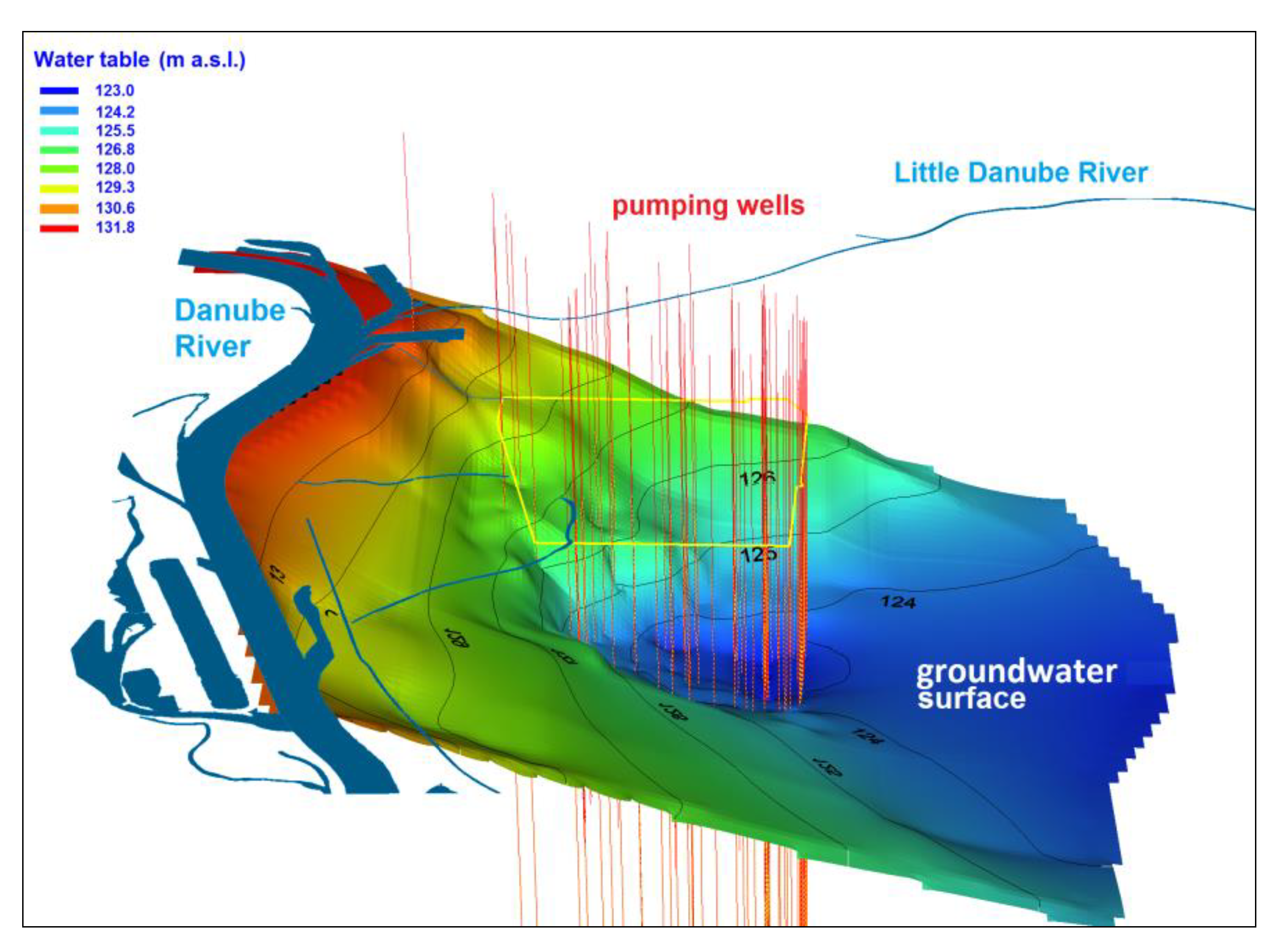
2.1. Model Settings
2.2. Model Calibration and Prediction
- OF: objective function (sum of squared residuals),
- HOB: groundwater head observations number,
- nPAR: number of adjusted parameters.
2.3. Conceptual Approach in Individual Model Scenarios
3. Results
4. Discussion
5. Conclusions
- -
- the K-field zonation based on groundwater level residuals’ distribution can be valuable in the calibration process if there are only limited K data from the field survey;
- -
- higher parametrization does not necessarily lead to a more effective solution regarding prediction accuracy and several variants of a solution with continual post-audit evaluation should be used whenever possible;
- -
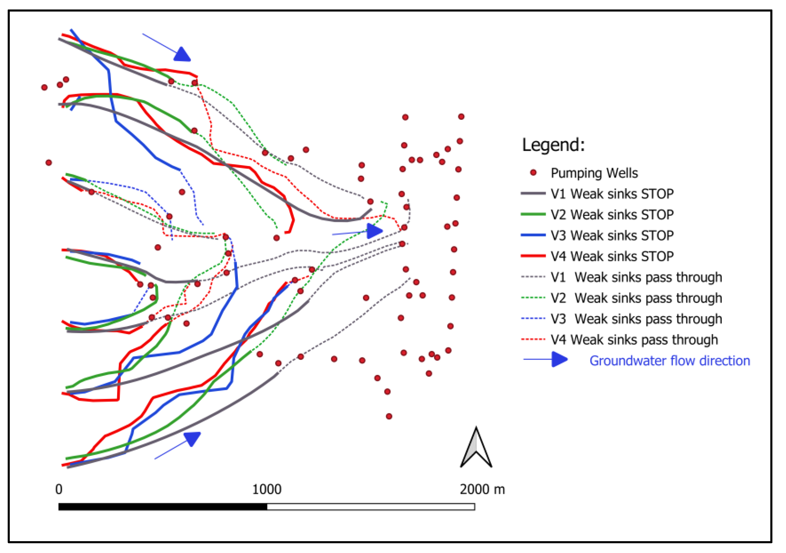
- different model variants with similar prediction accuracy in terms of groundwater level fit can produce different groundwater pathlines; and, finally,
- -
- the information criteria AIC, AICc, and BIC can be inaccurate in the evaluation of model prediction accuracy.
Author Contributions
Funding
Data Availability Statement
Acknowledgments
Conflicts of Interest
Abbreviations
| AIC | Akaike Information Criterion |
| AICc | Corrected Akaike Information Criterion |
| AVG | average |
| AVG ABS RES | averaged absolute residuals |
| BIC | Bayesian Information Criterion |
| E, W, N, S | east, west, north, south |
| EVT | evapotranspiration or evapotranspiration package/module in MODFLOW-2005 program |
| f | function |
| GLUE-MBA | Generalized Likelihood Uncertainty Estimation–Bayesian Model Averaging methods |
| GW | groundwater |
| GWHP | Groundwater Hydraulic Protection System |
| H | hydraulic head |
| CHD | Time-Variant Specified-Head package/module in MODFLOW-2005 program |
| K | hydraulic conductivity (m·s−1) |
| Kx, Ky | horizontal hydraulic conductivity (m·s−1) in “x” and “y” direction, respectively |
| Kz | vertical hydraulic conductivity (m·s−1) |
| LPF | layer property flow package/module in MODFLOW-2005 program |
| nPAR | number of adjusted parameters during calibration |
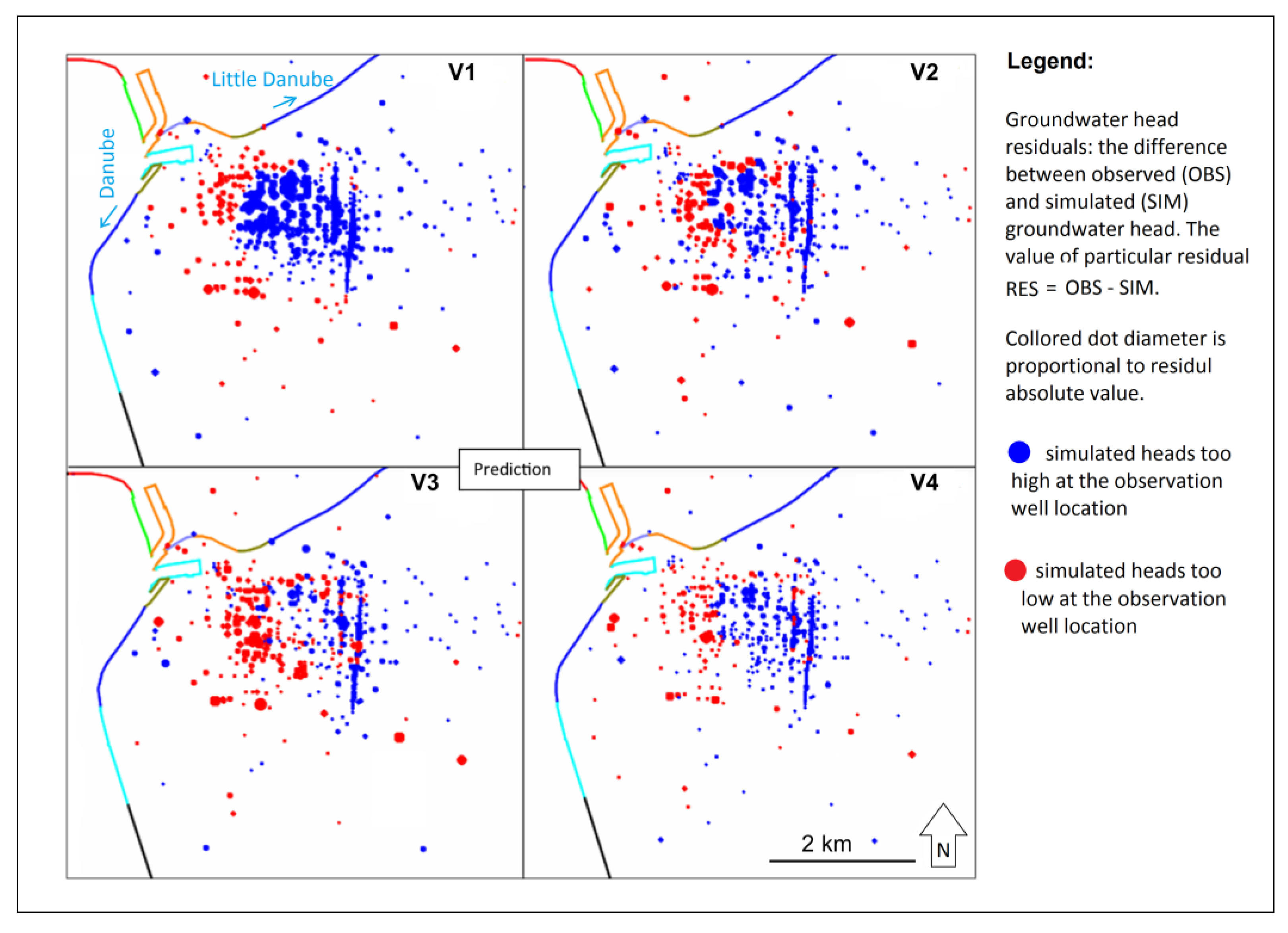
| OBS | observed groundwater head |
| OF | sum of squared residuals or objective function |
| PCG | preconditioned conjugate gradient package (solver) in MODFLOW-2005 program |
| Q | discharge or pumping rate (m3.s−1) |
| Q pump | overall pumping rate at modeled site |
| RES | groundwater head residual (difference between observed and simulated head) |
| RCH | recharge or recharge package/module in MODFLOW-2005 program |
| RIV | river package/module in MODFLOW-2005 program |
| RMSE | root mean square error |
| SIM | calculated (simulated) groundwater head |
| V1–V4 | model scenarios (variants) |
| WEL | well package/module in MODFLOW-2005 program |
References
- Poeter, E.P.; McKenna, S.A. Reducing uncertainty associated with groundwater flow and transport predictions. Groundwater 1995, 33, 899–904. [Google Scholar] [CrossRef]
- Poeter, E.P.; Hill, M.C. MMA, A Computer Code for Multi-Model Analysis; U.S. Geological Survey Techniques and Methods; USGS: Reston, VA, USA, 2007; 133p. [Google Scholar] [CrossRef]
- Refsgaard, J.C.; van der Sluijs, J.P.; Brown, J.; van der Keur, P. A framework for dealing with uncertainty due to model structure error. Adv. Water. Resour. 2006, 29, 1586–1597. [Google Scholar] [CrossRef]
- Akaike, H. A new look at statistical model identification. IEEE Trans. Autom. Control 1974, 19, 716–722. [Google Scholar] [CrossRef]
- Schwarz, G. Estimating the dimension of a model. Ann. Stat. 1978, 6, 461–464. [Google Scholar] [CrossRef]
- Hurvich, C.M.; Tsai, C.L. Regression and time series model selection in small sample. Biometrika 1989, 76, 297–307. [Google Scholar] [CrossRef]
- Emiliano, P.C.; Vivanco, M.J.F.; de Menezes, F.S. Information criteria: How do they behave in different models? Comput. Stat. Data Anal. 2014, 69, 141–153. [Google Scholar] [CrossRef]
- Singh, A.; Mishra, S.; Ruskauff, G. Model averaging techniques for quantifying conceptual model uncertainty. Groundwater 2010, 48, 701–715. [Google Scholar] [CrossRef]
- Ye, M.; Meyer, P.D.; Neuman, S.P. On model selection criteria in multimodel analysis. Water Resour. Res. 2008, 44, 1–12. [Google Scholar] [CrossRef]
- Poeter, E.P.; Anderson, D. Multimodel ranking and inference in ground water modeling. Groundwater 2005, 43, 597–605. [Google Scholar] [CrossRef]
- Massmann, C.; Birk, S.; Liedl, R.; Geyer, T. Identification of hydrogeological models: Application to tracer test analysis in a karst aquifer. In Calibration and Reliability in Groundwater Modelling: From Uncertainty to Decision Making, Proceedings of the ModelCARE’2005, The Hague, The Netherlands, 6–9 June 2005; IAHS Publ.: Wallingford, UK, 2006; Volume 304, pp. 59–64. [Google Scholar]
- De Aguinaga, J.G. Uncertainty Assessment of Hydrogeological Models Based on Information Theory. Ph.D. Thesis, Technische Universität Dresden, Dresden, Germany, 2010. [Google Scholar]
- Engelhardt, I.; De Aguinaga, J.G.; Mikat, H.; Schuth, C.; Liedl, R. Complexity vs. simplicity: Groundwater model ranking using information criteria. Groundwater 2014, 52, 573–583. [Google Scholar] [CrossRef]
- Foglia, L.; Mehl, S.W.; Hill, M.C.; Perona, P.; Burlando, P. Testing alternative ground water models using crossvalidation and other methods. Groundwater 2007, 45, 627–641. [Google Scholar] [CrossRef]
- Samani, S.; Moghaddam, A.A.; Ye, M. Investigating the effect of complexity on groundwater flow modeling uncertainty. Stoch Env. Res. Risk Assess 2018, 32, 643–659. [Google Scholar] [CrossRef]
- Anderson, M.P.; Woessner, W.W. The role of the postaudit in model validation. Adv. Water Resour. 1992, 15, 167–173. [Google Scholar] [CrossRef]
- Bredehoeft, J.D. From models to performance assessment—The conceptual problem. Groundwater 2003, 41, 571–577. [Google Scholar] [CrossRef]
- Konikow, L.F.; Bredehoeft, J.D. Ground-water models cannot be validated. Adv. Water Resour. 1992, 15, 75–83. [Google Scholar] [CrossRef]
- Hill, M.C. Methods and guidelines for effective model calibration. In U.S. Geological Survey Water-Resources Investigations Report; 98-4005; USGS: Reston, VA, USA, 1998. [Google Scholar] [CrossRef]
- Hill, M.C. The practical use of simplicity in developing ground water models. Groundwater 2006, 44, 775–781. [Google Scholar] [CrossRef] [PubMed]
- Clement, T.P. Complexities in hindcasting models: When should we say enough is enough. Groundwater 2010, 49, 620–629. [Google Scholar] [CrossRef] [PubMed]
- Cunge, J.A. Of data and models. J. Hydroinform. 2003, 5, 75–98. [Google Scholar] [CrossRef]
- Oreskes, N. The role of quantitative models in science. In Models in Ecosystem Science; Canham, C.D., Cole, J.J., Lauenroth, W.K., Eds.; Princeton University Press: Princeton, NJ, USA, 2003; pp. 13–31. [Google Scholar]
- Konikow, L.F. The secret to successful solute-transport modeling. Groundwater 2011, 49, 144–159. [Google Scholar] [CrossRef]
- Doherty, J. Modeling: Picture perfect or abstract art. Groundwater 2011, 49, 455–456. [Google Scholar] [CrossRef]
- Doherty, J.; Christensen, S. Use of paired simple and complex models to reduce predictive bias and quantify uncertainty. Water Resour. Res. 2011, 47, W12534. [Google Scholar] [CrossRef]
- Zatlakovič, M.; Augustovič, B.; Bugár, A.; Durdiaková, Ľ.; Gavuliaková, B.; Greš, P.; Guman, D.; Krebs, P.; Kuric, P.; Marenčák, Š.; et al. BRATISLAVA–SLOVNAFT XIII–Geological Survey and Remediation Works on Hydraulic Groundwater Protection in Upper Žitný Ostrov Area; Interim Report for 2019; VÚRUP, a.s.: Bratislava, Slovakia, 2020. [Google Scholar]
- Atlas krajiny SR (Atlas of Landscape of the Slovak Republic); MŽP SR: Bratislava, Slovakia, 2002.
- Harbaugh, A.W. MODFLOW-2005, the U.S. Geological Survey Modular Groundwater Model—The Ground-Water Flow Process; U.S. Geological Survey Techniques and Methods; USGS: Reston, VA, USA, 2005; Volume 6-A16. [CrossRef]
- Poeter, E.P.; Hill, M.C.; Banta, E.R.; Mehl, S.; Christensen, S. UCODE_2005 and Six Other Computer Codes for Universal Sensitivity Analysis, Calibration, and Uncertainty Evaluation Constructed Using the JUPITER API; U.S. Geological Survey Techniques and Methods; USGS: Reston, VA, USA, 2005; chap. A11, bk. 6. [CrossRef]
- Pollock, D.W. User Guide for MODPATH Version 6, a Particle-Tracking Model for MODFLOW; U. S. Geological Survey Techniques and Methods; USGS: Reston, VA, USA, 2012; Volume 6-A41, 58p. [CrossRef]
- Carrera, J.; Neuman, S.P. Estimation of aquifer parameters under transient and steady-state conditions. Water Resour. Res. 1986, 22, 199–242. [Google Scholar] [CrossRef]
- Moore, C.; Doherty, J. The cost of uniqueness in groundwater model calibration. Adv. Water Resour. 2006, 29, 605–623. [Google Scholar] [CrossRef]
- Hunt, R.J.; Welter, D.E. Taking account of “unknown unknowns”. Groundwater 2010, 48, 477. [Google Scholar] [CrossRef]
- Rojas, R.; Batelaan, O.; Feyen, L.; Dassargues, A. Assessment of conceptual model uncertainty for the regional aquifer Pampa del Tamarugal, North Chile. Hydrol. Earth Syst. Sci. 2010, 14, 171–192. [Google Scholar] [CrossRef]
- Troldborg, L.; Refsgaard, J.C.; Jensen, K.H.; Engesgaard, P. The importance of alternative conceptual models for simulation of concentrations in multi-aquifer system. Hydrogeol. J. 2007, 15, 843–860. [Google Scholar] [CrossRef]
- Cooley, R.L. A Theory for Modeling Ground-Water Flow in Heterogeneous Media; U.S. Geological Survey professional paper 1679; USGS: Reston, VA, USA, 2004. [CrossRef]
- Moore, C.; Doherty, J. The role of the calibration process in reducing model predictive error. Water Resour. Res. 2005, 41, W05020. [Google Scholar] [CrossRef]


| Feature | Units | 2008 | 2019 | ABS Delta |
|---|---|---|---|---|
| AVG OBS | m a.s.l. | 124.27 | 123.69 | 0.58 |
| AVG RIV 1 | m a.s.l. | 131.83 | 131.99 | 0.16 |
| AVG RIV 2 | m a.s.l. | 130.91 | 130.87 | 0.04 |
| AVG Q pumping | m3·s−1 | 0.916 | 1.009 | 0.093 |
| Model Variant | nPAR | OF | AVG RES (m) | AVG ABS RES (m) | RMSE (m) | AIC | AICc | BIC | RMSE and OBS Dispersion Ratio (%) |
|---|---|---|---|---|---|---|---|---|---|
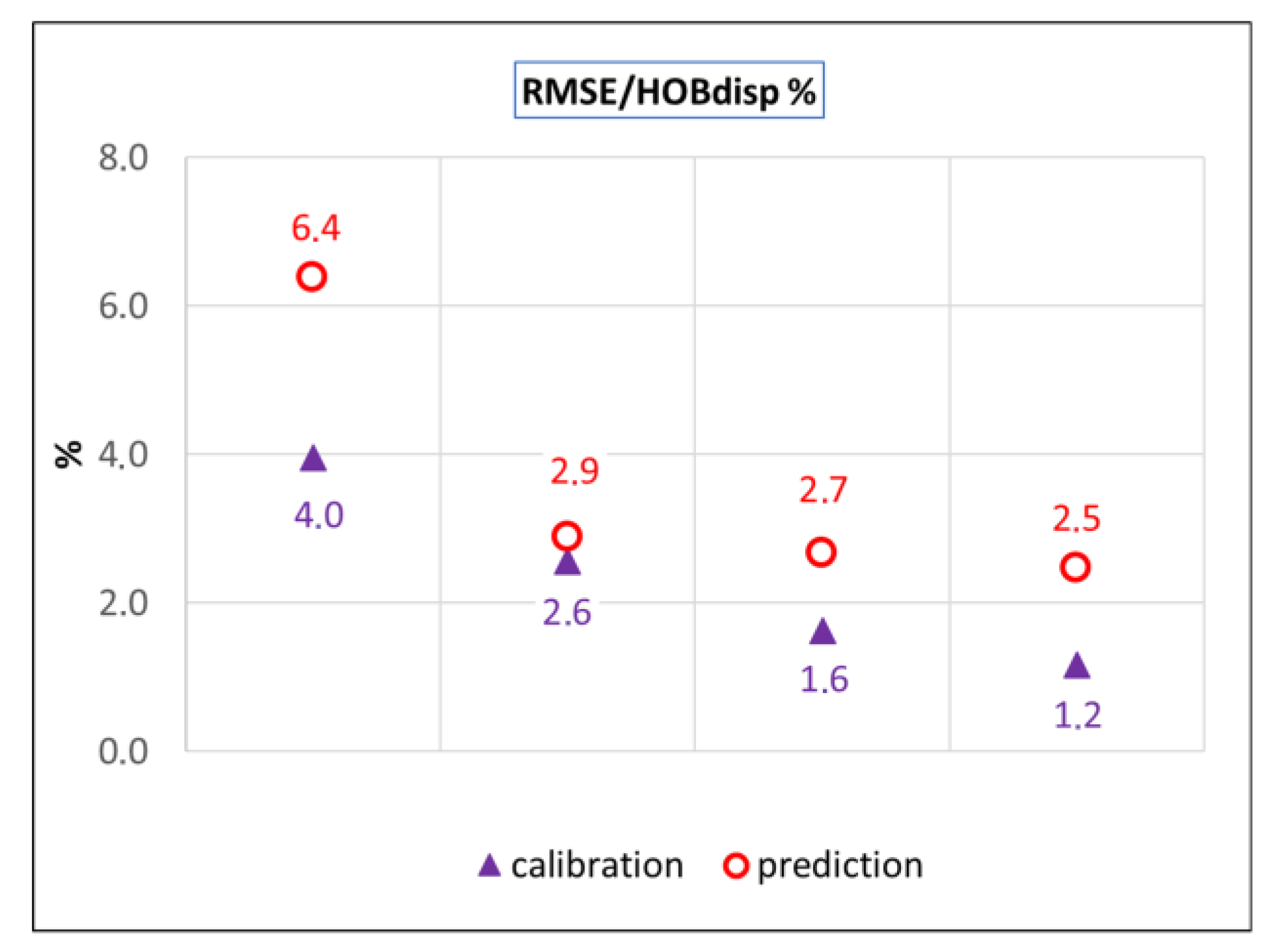
| V1 | 2 | 64.5 | 0.04 | 0.25 | 0.34 | 69 | 69 | 77 | 4.0 |
| V2 | 43 | 26.5 | −0.05 | 0.14 | 0.22 | 113 | 121 | 298 | 2.6 |
| V3 | 139 | 11.0 | 0.05 | 0.11 | 0.14 | 289 | 389 | 885 | 1.6 |
| V4 | 255 | 5.8 | −0.01 | 0.07 | 0.1 | 516 | 977 | 1611 | 1.2 |
| Model Variant | OF | AVG RES (m) | AVG ABS RES (m) | RMSE (m) | RMSE and OBS Dispersion Ratio (%) |
|---|---|---|---|---|---|
| V1_2019 | 205.7 | −0.29 | 0.45 | 0.62 | 6.4 |
| V2_2019 | 44.2 | −0.05 | 0.20 | 0.28 | 2.9 |
| V3_2019 | 35.7 | 0.03 | 0.17 | 0.26 | 2.7 |
| V4_2019 | 31.4 | −0.06 | 0.17 | 0.24 | 2.5 |
Disclaimer/Publisher’s Note: The statements, opinions and data contained in all publications are solely those of the individual author(s) and contributor(s) and not of MDPI and/or the editor(s). MDPI and/or the editor(s) disclaim responsibility for any injury to people or property resulting from any ideas, methods, instructions or products referred to in the content. |
© 2023 by the authors. Licensee MDPI, Basel, Switzerland. This article is an open access article distributed under the terms and conditions of the Creative Commons Attribution (CC BY) license (https://creativecommons.org/licenses/by/4.0/).
Share and Cite
Zatlakovič, M.; Krčmář, D.; Hodasová, K.; Sracek, O.; Marenčák, Š.; Durdiaková, Ľ.; Bugár, A. The Impact of Groundwater Model Parametrization on Calibration Fit and Prediction Accuracy—Assessment in the Form of a Post-Audit at the SLOVNAFT Oil Refinery Site, in Slovakia. Water 2023, 15, 839. https://doi.org/10.3390/w15050839
Zatlakovič M, Krčmář D, Hodasová K, Sracek O, Marenčák Š, Durdiaková Ľ, Bugár A. The Impact of Groundwater Model Parametrization on Calibration Fit and Prediction Accuracy—Assessment in the Form of a Post-Audit at the SLOVNAFT Oil Refinery Site, in Slovakia. Water. 2023; 15(5):839. https://doi.org/10.3390/w15050839
Chicago/Turabian StyleZatlakovič, Martin, Dávid Krčmář, Kamila Hodasová, Ondra Sracek, Štefan Marenčák, Ľubica Durdiaková, and Alexander Bugár. 2023. "The Impact of Groundwater Model Parametrization on Calibration Fit and Prediction Accuracy—Assessment in the Form of a Post-Audit at the SLOVNAFT Oil Refinery Site, in Slovakia" Water 15, no. 5: 839. https://doi.org/10.3390/w15050839
APA StyleZatlakovič, M., Krčmář, D., Hodasová, K., Sracek, O., Marenčák, Š., Durdiaková, Ľ., & Bugár, A. (2023). The Impact of Groundwater Model Parametrization on Calibration Fit and Prediction Accuracy—Assessment in the Form of a Post-Audit at the SLOVNAFT Oil Refinery Site, in Slovakia. Water, 15(5), 839. https://doi.org/10.3390/w15050839