Algorithm for Appropriate Design of Hydroelectric Turbines as Replacements for Pressure Reduction Valves in Water Distribution Systems

Abstract

Gravity flow water distribution systems (WDSs) are used to permit water flow from an input point of highest elevation (source) to the terminal points of a system (consumers). In such WDSs, typically, there is no need for external power to maintain the flow due to the typical high gradients that exist. However, those gradients cause high water velocity and pressure to some network areas that could potentially lead to pipes bursting. Currently, the only means to regulate pressure within allowable range are Pressure Reduction Valves (PRVs). They are installed at various locations, but they cannot utilize the existing hydropower potential in terms of electrical energy production. This paper provides a methodology for hydro-turbines dimensioning, so that they mimic PRV operation in terms of pressure regulation while producing power efficiently. This includes an algorithmic process within which the proper turbine design and performance prediction are initially determined, and then, via an interconnection between EPANET and MATLAB, the hydraulic behavior of their operation within the water network is modeled and simulated. The methodology has been tested with simulations of a typical urban WDS. The results indicate that the produced turbine geometries mimic PRV action at the respective locations with more than 1% accuracy during 70% of the time (2% maximum error), while producing electric energy with hydraulic efficiency over 60%.

1. Introduction

Since ancient times, water has constituted a unique source of energy that was used systematically in favor of man’s interests. It is practically inexhaustible and considered among the clean forms of energy which, if exploited, could lead to the production of substantial amounts of low-cost electrical energy. All contemporary Water Distribution Systems (WDSs) contain a significant amount of such energy. In gravity systems the input point of the main tank is higher than all the withdrawal points, so there is no need for a pumping system for water flow circulation [1]. Consequently, due to this significant elevation difference, within the lower parts of the network a high water pressure is witnessed that needs to be reduced for pipeline and consumer safety. Unfortunately, this means that even today we dissipate a significant amount of green energy in order to abide by the hydraulic restrictions of the network and consumer comfort.

At the same time, existing WDSs do not incorporate efficient strategies for achieving water savings through water demand control, while corresponding methods towards this direction still have not been extensively researched [2]. Achieving a significant amount of water savings by introducing technical methods for preventing consumer prodigality is not only considered valuable from an environmental standpoint (i.e., water conservation), but also from an economic one. Furthermore, the restriction of end-side demand to a lower, but sufficient, value reduces water leakages and losses as they are both proportional to pipe water flow. Poor WDS infrastructure and restricted budgets lead to water supply inefficiency [3] and significant annual water losses that bear a significant cost for water utilities, which is eventually rolled over to consumers. One of the most common and efficient techniques to minimize water losses and leakages is water pressure reduction [4,5].

In practice, pressure regulation is usually achieved by common hydraulic structures and devices like Brake-Pressure Tanks (BPTs), where the excess hydrostatic pressure and kinetic energy of water is dissipated to the atmospheric pressure and Pressure Reduction Valves (PRVs) [6,7,8] that can regulate the downstream water pressure to the desired (set) value. These mechanisms keep water pressure within reasonable range, and thus, minimize the risk of pipeline bursts and service inconvenience. Despite their simple construction and operation, PRVs are especially prone to failures due to the mechanical elements that they consist of and require frequent maintenance to ensure that they work efficiently. At the same time, both BPTs and PRVs are considered as passive devices that achieve pressure adjustment only in one direction, i.e., at their outlet, while not having the ability to utilize any of the water energy at their inlet. Recent research recommends the use of Pumps As Turbines (PATs) as the standard energy recovery machines [9,10,11,12]. They combine simple and cost-effective operation when optimally selected and located in a WDS [9,11]. Many correlation methods, empirical expressions and approach equations have been proposed to assess the Best Efficiency Point (BEP) of the PAT and to improve its performance during variable operation strategies [10,12,13,14,15]. Unfortunately, their employment is accompanied by uncertainty in performance prediction, lower efficiency and inflexibility in ranging operational conditions [12,13,16]. Therefore, this work is part of ongoing research that investigates the alternative solution in WDSs of the more expensive, but well-documented and efficient, turbines [17,18]. The installation of a hydro-turbine that converts the excess energy of PRVs in terms of pressure head into useful energy in the form of electricity appears as a promising alternative in many research papers [19,20,21,22,23]. In particular, the techno-economic feasibility and environmental benefits that derive from this renewable energy production are outlined in [19,20,21], while the assessment of the energy potential in such systems is demonstrated in [19,20,21,22]. An analytical study for optimal location selection of PRVs and hydro-turbines in WDSs can be found in [23,24], while the economic viability of turbines placed in municipal water networks is highlighted in [25].

Hydro-generation from WDSs constitutes a unique case of Renewable Energy Source (RES) that sets it apart from all the typical RESs, especially photovoltaics and wind turbines, in four notable ways: Firstly, there is no overreliance between the weather conditions and the water demand. This in turn translates into two beneficiary outcomes. Initially, the expected hydro-turbine power generation can be estimated with high accuracy because the water discharge is dependent on the consumption [19], unlike the solar and wind power generation that are associated with uncertainty and relative unpredictability. Secondly, power generation from water can be produced non-stop. On the contrary, photovoltaic generation is insignificant during extreme cloud cover conditions or even zero at night, while wind turbines cannot produce power during low wind speeds. Furthermore, the hydro-turbine installation in a WDS is practically invisible, as it employs network infrastructure and components that are already in use [20], does not occupy land, and therefore does not have an aesthetic impact or constitute a public nuisance, unlike the wind and solar projects that can, at times, cause unreasonable discomfort or annoyance to neighboring landowners and the general public. More specifically, wind turbines produce noise at short distances and demand significant supportive construction, while residential solar panels, due to their low kWp/m² ratio, occupy large surfaces on rooftops to achieve a respectable amount of power output. Finally, the energy provided by hydro-turbine installations in WDSs is produced and mostly consumed locally as it is reasonable to assume that population density, water consumption and electricity demand are correlated [26,27].

Many researchers investigate the economic benefit of replacing PRVs with recovery machines, but their perspective is limited to dissipated energy. To the best of our knowledge, there is currently no published work on proper dimensioning and design of recovery machines that achieve identical downstream pressure as PRVs. This work aims to provide a step-by-step methodology for dimensioning turbines planned to replace the existing PRVs in a typical WDS. The implementation of the suggested algorithmic process allows minimum deviation between the PRV and turbine operation in terms of achieved downstream pressure through the proper sizing and performance prediction of hydro-turbine units. Considering that the current methodology targets at precisely mimicking PRV operation, water losses achieved by turbine operation are expected to be the same as the PRVs. In addition, the hydro-turbine’s ability for pressure regulation is assessed and its performance in producing clean electric energy is evaluated. In this paper, a WDS obtained from the Kentucky Infrastructure Utility (KIA) is used as a case study [28]. Its hydraulic behavior is simulated with the use of EPANET, the industry standard software. To investigate the accuracy and credibility of the results, the default demand-driven method is adopted in order to solve the existent network model. The target is to test the ability of the suggested hydro-turbine designs to achieve pressure regulation similar to PRVs and power generation.

The structure of this paper is as follows: The required background is presented in Section 2, divided into three parts. First, the basic hydro-turbine design and performance principles are introduced. Later, the features and differences in the standard simulation models that are used in contemporary WDS are presented. Lastly, the simulation tools EPANET and EPANET-MATLAB Toolkit are presented.

In the third section, after describing the general WDS layout, the dimensioning process for a hydro-turbine located at a specific network point is discussed and the methodology that is used during hydro-turbine simulation within the robust model of EPANET is explained.

In the fourth section, the results derived from the proper turbine dimensioning on several locations of a typical WDS are presented and discussed, followed by the evaluation of hydro-turbine’s performance in both pressure regulation and energy production.

In the concluding section, the total impact of properly sized hydro-turbines installed in a WDS is summarized. The prospect that emerges in water pressure management and alternative power generation is also discussed, and finally, future research possibilities are being suggested.

2. Background

2.1. Hydro-Turbine Performance-Characteristic H–Q Curves

The aim of this work is to provide the guidelines for proper dimensioning of hydro-turbines installed in a WDS, and the estimation of their performance. At the start of every preliminary hydro-turbine design process and performance prediction it is mandatory to calculate the specific speed, i.e., a rating for hydro-turbine performance. In this paper, the dimensional specific speed formula is adopted. It involves all operating conditions: volumetric flow rate (Q), turbine working head (H) and runner rotational speed (N), i.e.:

$$n_q=\frac{N·\sqrt{Q}}{H^{0.75}}$$

(1)

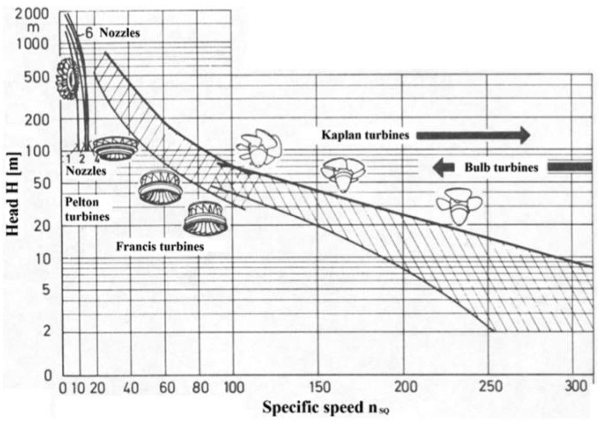
The calculation of specific speed enables us to make use of various correlation diagrams derived from published experimental data that indicate the optimal hydraulic profile of a turbine. Important design and operating parameters, like turbine type and main dimensioning, hub-to-tip diameter ratio, number of blades, work coefficients and even an estimation of hydraulic efficiency, result from their correlation with specific speed. This allows us to have a good first estimation of turbine sizing and performance without the need for in-depth analysis. A typical correlation diagram that involves specific speed, head and turbine type selection is shown in Figure 1.

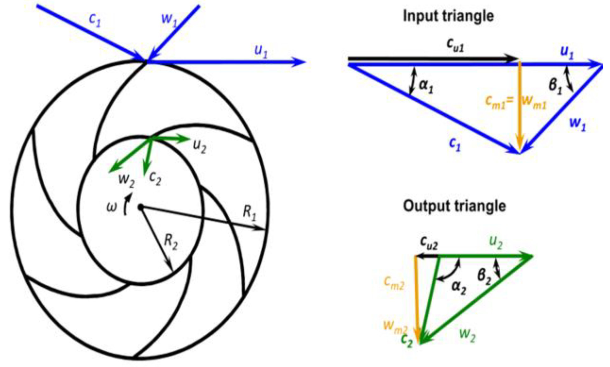
A combination of specific values for Q (m³/s), N (rpm) and H (m) determines the so-called “design point” or Best Efficiency Point (BEP) of the hydro-turbine, i.e., the point where the hydro-turbine is designed to operate at its highest efficiency. Euler’s fundamental equation for turbines relates the power absorbed from the water flow with the geometry and the velocities of the runner. Its general formulation is presented in Equation (2a). By rearranging Equation (2a) by means of introducing the geometrical properties of the runner, its mathematical formula shapes into Equation (2b). Equation (2b) applies to all reaction type turbines and becomes more accurate when blade thickness can be assumed negligible when compared with the annulus passage area over the entire blade zone [30]. The schematic representation of the velocity triangles at turbine inlet and outlet, along with the notation of the various velocity components and angles that are employed in Equation (2) are depicted in Figure 2.

$$H_{Euler}=H_{des}=\frac{(C_{u1}·u_1-C_{u2}·u_2)}{g}$$

(2a)

$$H_{des}=f\left(Q_{des}\right)=\frac{u_2·Q_{des}}{g}\left(\frac{1}{\pi D_2{b}_1 }·\frac{1}{tg{\alpha }_1 }+\frac{1}{\pi D_2{b}_2 }·\frac{1}{tg{\beta }_2 }\right)-\frac{u_2^2}{g}$$

(2b)

where: g is the gravitational acceleration (m/s²);

c_u1, c_u2 is the tangential component of the absolute blade velocity at turbine inlet and outlet velocity triangles (m/s);

Q_des is the design flow rate (m³/s);

u₁, u₂ are the peripheral blade velocity at turbine inlet and outlet velocity triangles (m/s);

D₂ is the outlet runner diameter (m);

b₁, b₂ are the inlet and outlet blade width (m);

α₁ is the guide vane’s pre-swirl angle (in degrees);

β₂ is the blade outlet angle (in degrees).

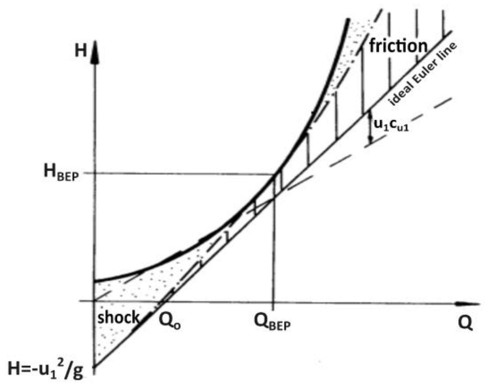
In many cases, hydro-turbines are required to operate in conditions and scenarios away from their design point: different flow rate, head and power output. In practice, to handle efficiently different operating conditions (e.g., suboptimal water flow rates), reaction turbines like Francis or Kaplan are always equipped with guide vanes. In the case of Kaplan an adjustable runner blade angle mechanism is also added. Guide vanes, specifically, consist of several blades that can be adjusted to guide the water flow through the runner blades in an optimal angle (i.e., shockless entry). For a hydro-turbine to keep working efficiently, either in terms of achieving its power output with maximum efficiency or imposing a specific head drop regardless of the efficiency, as is required by the operation of PRVs, it is necessary to estimate all corresponding working points. This is possible by constructing both the η–Q (efficiency-flow rate) curve and the characteristic H–Q (head-flow rate) curve, which indicate the way that efficiency and head change with varying flow rate, respectively. Normally, the H–Q curve is a strictly increasing function, as it is showcased in Figure 3 [32] and becomes evident from Equation (2b) by calculating H as a function of Q. Such curves can be drawn for a specific rotational speed value and absolute flow angle at inlet, which in turn depends on guide vane opening. From the ideal Euler line it can be observed that for each such curve there is always a critical flow rate (Q_o) below which the hydro-turbine does not work as intended, but enters a mode of operation where it behaves neither as turbine nor as pump [33]. By changing the absolute flow angle at inlet to a bounded range and forming the equivalent η–Q and H–Q curves, the behavior of the same machine for different operating points (flow rates, heads and rotational speeds) can be assessed. Equation (3) suggests that the final characteristic H–Q curve, also known as the actual performance curve, results from the ideal Euler line if all forms of losses (i.e., hydraulic, volumetric, kinetic) are included. In practice, hydraulic losses (i.e., friction and shock losses) are the most consequential, and hence it is essential to introduce their mathematical expressions by Equations (4) and (5). Then, the hydraulic efficiency which accounts for these losses is calculated in Equation (6).

$$H_{actual}=H_{ideal}+H_{losses}$$

(3)

$$\delta h_{shock}={\zeta }_s·\left(1-\frac{Q_i}{Q_{des}}\right)·\frac{u_1^2}{2g}$$

(4)

$$\delta h_{friction}={\zeta }_f·Q^2$$

(5)

$${\eta }_h=\frac{H_{\mathrm{Euler}}}{H_{\mathrm{actual}}}=\frac{H_{\mathrm{des}}}{H_{\mathrm{actual}}}=\frac{(C_{u1}·u_1-C_{u2}·u_2)}{g·H_{\mathrm{actual}}}$$

(6)

where: Q_i is the flow value away from the design point (m³/s);

η_h is the hydraulic efficiency;

ζ_s and ζ_f are the shock and friction loss coefficients; respectively.

Τhe coefficient ζ_s ranges between 0.5 and 0.7 [34] and ζ_f includes the combined effect of both major (friction) and minor losses; their values are calculated in such a way that the actual curve of the estimated efficiency will cross the design point according to turbine and blade shape and structure. In practice, these various losses tend to generate characteristics whose maximum efficiency is reached at water flow values lower than the original design flow.

According to Equations (4) and (5), for constant u₁ and since coefficients ζ_f, and ζ_s are considered constant at the fully turbulent region, hydraulic and shock losses are dependent solely on the flow [33].

2.2. Similarity Laws

According to laws of similarity, during conditions of dynamic similarity of flow it can be proven that between different working points the following set of simplifying equations are satisfied [33,35]:

$$\frac{Q_1}{Q_2}={\left(\frac{D_1}{D_2}\right)}^3·\frac{N_1}{N_2}$$

(7)

$$\frac{H_1}{H_2}={\left(\frac{D_1}{D_2}\right)}^2·{\left(\frac{N_1}{N_2}\right)}^2$$

(8)

$$\frac{P_1}{P_2}={\left(\frac{D_1}{D_2}\right)}^5·{\left(\frac{N_1}{N_2}\right)}^3$$

(9)

where: N₁ and N₂ represent different runner rotational speeds (rpm);

Q₁ and Q₂ are the flow rates at speed N₁ and N₂, respectively (m³/s);

H₁ and H₂ are turbine heads at speed N₁ and N₂, respectively (m);

P₁ and P₂ are the mechanical power outputs at speed N₁ and N₂, respectively (kW);

D₁ and D₂ represent the tip diameters of two different turbines (m).

If the behavior of the same hydro-turbine is to be assessed, i.e., D₁ = D₂ = constant at different operational conditions, then Equations (7)–(9) are grouped together into Εquation (10):

$$\frac{Q_1}{Q_2}=\frac{N_1}{N_2}={\left(\frac{H_1}{H_2}\right)}^{\frac{1}{2}}$$

(10)

By assuming coefficients ζ_h, ζ_s as constant (see Section 2.1), losses in head δh_hydraulic and δh_shock can be computed for different operating conditions (Q₂, N_2, H₂, η₂), with respect to the initial design (Q₁, N_1, H₁, η₁), as follows:

$$\frac{Q_1}{Q_2}=\frac{N_1}{N_2}={\left(\frac{H_1}{H_2}\right)}^{\frac{1}{2}}={\left(\frac{\delta h_1{}^{hydraulic}}{\delta h_2{}^{hydraulic}}\right)}^{\frac{1}{2}}={\left(\frac{\delta h_1{}^{shock}}{\delta h_2{}^{shock}}\right)}^{\frac{1}{2}}$$

(11)

In practice, efficiency is assumed to remain unchanged for speed variations less than 20%, i.e., $\frac{N_1-N_2}{N_2}·100\%$< 20%, while for larger variations a corrective factor is applied [33]:

$${\eta }_2=1-\left(1-{\eta }_1\right)·{\left(\frac{N_1}{N_2}\right)}^{0.1}$$

(12)

where η₂ is the total efficiency for rotational speed N_2, while η₁ represents the total efficiency of the corresponding working point for rotational speed N₁.

By deploying the characteristic H–Q curve and similarity laws it is possible to switch between different H–Q curves (see Section 2.4) and treat the given hydro-turbine in two ways:

• As a power generating machine by focusing on the working points which, according to the current flow rate, maintain the maximum efficiency regardless of the resulting head-pressure drop at the outlet;
• As a water pressure regulator that keeps track of the working points that achieve the requested head-pressure drop at its outlet with the available flow rate, regardless of the resulting efficiency or power output.

Therefore, turbine operation settings (turbine rotational speed, guide vane opening and water pressure) can be used as variables in an optimization process for different objectives that consider water network constraints, such as maximum power generation, precise pressure regulation and minimization of water losses. In the present paper only the hydro-turbine’s performance as water pressure regulator is being investigated. Electric power generation is calculated only as a byproduct of the pressure regulation process.

2.3. Simulation Approach

Hydraulic modeling and simulation software, like EPANET [36], are based on Demand-Driven Analysis (DDA). The DDA approach assumes that nodal water inflow has a fixed and known value. This means that nodal water demand remains constant and is always fully satisfied, irrespective of the available nodal hydraulic head, a condition that can be accurate only when every system location works under normal conditions and the required nodal pressure is satisfied [37]. This means that in a DDA model the consumer will always be supplied, and demands will always be met, even if pressure drops below a physically realistic level, i.e., nodal pressure head becomes lower than required consumer’s head or even negative. It is not uncommon that occasions like high demand for fire-fighting, pipe bursts or failures and demands in excess of design capacity can lead to pressure insufficiency [38]. It is obvious that in such scenarios, employing a DDA model may lead to misleading results concerning network reliability and redundancy, regardless of the iterative algorithm it uses to solve the system equations.

Nevertheless, DDA models simulate system behavior accurately if the system rarely enters an abnormal condition, which is clearly the case with well-designed water networks. Consequently, the majority of modern hydraulic simulation applications are based on DDA. Pressure-Driven Analysis (PDA) is engaged only in “abnormal” conditions scenarios. Then, water demand is not only a function of time, but also a function of pressure [39,40,41]. For a WDS model to be realistic it should be able to accommodate both pressure independent and pressure controlled demand, which is the case with EPANET as it enables the user to run both a DDA and PDA simulation depending on network conditions. In this paper, network behavior during regular operating conditions is being assessed, and hence, the typical DDA model is adopted.

EPANET is considered the industry standard software for extended time period simulations of the hydraulic behavior of water distribution networks. It implements the conventional DDA approach, and the system equations are solved according to the Global Gradient Method [42,43]. The Global Gradient Method’s wide acceptance and success has led to various modifications, extensions and alternative formulations in order to further improve the already good convergence characteristics and robustness [44,45]. However, for the scope of this work EPANET’s default solution method is considered “sufficient”.

In this work, an external algorithm has been created in MATLAB to calculate the turbine’s main geometry followed by its performance prediction. According to these two key aspects, all the characteristic H–Q curves for the different scenarios are created, which in turn are imported on the EPANET network via the EPANET-MATLAB toolkit. EPANET-MATLAB Toolkit [46] operates within the MATLAB environment and provides a programming interface within EPANET, allowing access to all its shared object libraries and executables. This enables MATLAB to directly call EPANET’s dynamic-link library, have access to all network information, as well as to be able to modify and visualize its topology and simulate its hydraulic behavior.

EPANET is able to incorporate and model hydro-turbine operation within its workspace [36,47], which is done with the proper adjustment of the parameters of the General Purpose Valve (GPV) model. It requests as an input the GPV’s diameter, which in the context of this paper matches the turbine’s tip diameter, and as a setting it requests its flow-head relationship. This relationship is expressed by the characteristic H–Q curve that represents the turbine’s performance curve, i.e., the pressure head drop H that it imposes at its outlet with changing volumetric flow rate Q at its inlet. With the use of EPANET-MATLAB-toolkit, the GPV settings can be adjusted “on the fly”, as they are calculated off-line using MATLAB, by importing a new H–Q curve in order to impose a different pressure drop on the turbine’s outlet. Of course, this curve must represent the equivalent performance curve of the same turbine that corresponds to the adapted conditions. In this way, the turbine’s behavior can adapt to the changing operating conditions of the water network with the adjustment of the turbine’s rotational speed, guide vane opening and blade angles in a bounded range. The adaptation provides control over pressure regulation, power generation and efficiency.

2.4. Hydro-Turbine Realistic Design

As was discussed in the previous section, EPANET and EPANET-MATLAB-toolkit, simulate hydro-turbines’ behavior based on a turbine’s outer diameter and its characteristic H–Q performance curve. By modifying any of these fields the turbine’s operation will change as well. If the installation of a certain turbine of given diameter is decided, the only parameters that can be modified in a bounded range are its rotational speed, the guide vane opening and runner blade angles. Adjusting solely the rotational speed leads to a much simpler control mechanism, but restricts the range of head loss that can be achieved. Therefore, it restrains the turbine’s ability to replace an existing PRV that naturally handles a wide range of pressure-head values. In contrast, by being able to adjust both rotational speed and the angle at which the water impacts the fixed runner blades, the range of the attainable head loss is widely expanded but at the cost of a more complicated geometry and the need of additional moving parts. Depending on the hydro-turbine machine type, those moving parts can include moving guide vanes and fixed runner blades (single-regulated) in the case of a radial flow hydro-turbine (Francis type), or moving guide vanes and adjustable runner blades (double-regulated) in the cases of mixed and axial flow turbines (Deriaz and Kaplan types) (see Figure 1).

The hydro-turbine type that will be finally chosen will be determined mainly by its capability to provide PRV services during fluctuant flow rate and head. However, it is essential that the final hydro-turbine geometry is as simple, robust and cheap as possible. In this work, a radial flow hydro-turbine, a Francis type specifically, is always assumed to be the case due to the following facts:

• Traditionally, impulse turbines like Pelton or Turgo are inadequate for PRV replacement because their runner is not submerged in water, and they provide atmospheric pressure outflow (not controllable). Crossflow turbines can reduce water velocity, but they have extremely limited capability to reduce head [48];
• The expected water intake Q is rather limited in the case of WDSs. Radial turbines tend to work more efficiently than Kaplan turbines in such flows;
• In practice, PRVs installed in WDSs reduce the pressure by 1–10 bars (≈10–100 m of Head), which ranges within the Francis region as it is depicted in Figure 1;
• Francis hydro-turbines, among all other types, have the ability to cover the widest range of heads and volumetric flows;
• Francis turbines are single-regulated, and thus, compared to double-regulated axial type turbines like Kaplan, present a robust, economical and less complicated alternative in terms of runner and generator construction.

The combinations of relatively small water flows Q and high heads H result in small n_q values and thus lead towards the radial flow hydro-turbine region, which typically ranges between 20 and 80 (see Figure 1). The selection of Francis turbines among turbine types based on the specific speeds between 20 and 80 is a straightforward process, and is justified by classic hydropower analysis. All experimental results and Computational Fluid Dynamic (CFD) simulations indicate that turbine type selection and design based on n_q leads to the best performance-highest efficiency.

However, recent research that focuses on energy harvesting methods in WDSs has recommended the alternative of employing PAT systems. Comparing Francis turbines with PATs is not as simple as comparing different turbine types, and thus additional practical, economical and performance aspects need to be considered. The considerable performance, its mass availability and reduced cost indicate that a PAT system is a promising option for cheap and efficient energy recovery in micro-scale models [13]. However, its employment presents two major disadvantages. Firstly, since PATs do not possess an adjustable guide vane mechanism their adaptability in fluctuating flow rates and head is rather limited, and thus the combined employment of hydraulic and electrical regulation is always required [9]. However, even then they are not able to cover a wide operating range, as the Francis turbines do [12], and ultimately, they cannot be considered appropriate devices for PRV replacement. Secondly, since PAT technology is not as well documented as turbines, the determination of their BEP when operating as turbines still presents a major challenge [14]. Furthermore, their overall performance prediction contains significant uncertainty [16]. PATs are effective mainly when used in locations with low water demand variation [11], which are difficult to pinpoint a priori and are unlikely to be encountered in PRV sites [49]; thus, the location alternatives under which their installation can be economically justified is rather limited.

Flow rate and head continually fluctuate in WDSs and PRVs upstream. Furthermore, in a WDS the impact of each interfering action needs to be well supported by both experimental and CFD results beforehand. Therefore, the employment of Francis turbines leads to a more flexible, efficient and well-founded solution for ultimately matching the PRV operation. Particularly in transient flow cases, there are strong indications that micro-turbines have the potential to offer an even better pressure regulation than PRVs [50]. In fact, in WDS locations with the great energy potential (>10 kW) that appears in large pipes (>200 mm), the cost of installing turbines instead of PATs [51] or even PRVs [52] becomes comparable. For all the above reasons a Francis type hydro-turbine is selected.

3. Methodology, Turbine Installation and Network Simulation

3.1. General Methodology

The hydro-turbine’s performance is being assessed by replacing the PRVs with their equivalent GPVs acting as turbines and the corresponding H–Q curves as settings. Hence, at first, it is vital to determine the PRVs operating modes at each period of time. In general, PRVs present two operating modes:

• Active, by keeping the downstream pressure to its setting value when the upstream pressure is higher than this setting value;
• Inactive, if the downstream pressure is lower than its setting value.

The exact working periods of the turbines are identical with the time periods that the PRVs are active, since they both aim at regulating pressure at a predetermined threshold.

Next, GPV/turbine’s diameter and its design point need to be assigned. Each GPV/turbine diameter should match the existing pipeline system diameter that the turbine is planned to be installed. The specific speed, and hence the design point determination, for each turbine is based on the average flow rate of each pipe Q, on the corresponding head loss range H that is required in order to fully replicate PRVs impact on downstream water pressure and, finally, on the corresponding runner rotational speed N. This triad of values is selected in such a way that the given tip diameter always correlates to the design point of the actual turbine. In this paper, without limiting the generality of the methodology, the selected upper speed limit is considered 4500 rpm and is assumed to be regulated by the operation of the generator coupled with the turbine. Direct drive synchronous generators that are used for variable speed applications, like the suggested one, require power converters that guarantee that the output power and water pressure are controlled in real time in such a way that the synchronization with the power grid is secured. Therefore, varying speed and speeds up to 4500 rpm can be handled by the converters. For all the above reasons, before determining a turbine’s main dimensioning and design point it is mandatory to collect information concerning the operating conditions and hydraulic properties of the network, such as:

• PRV active periods;
• Head and pressure values of the upstream and downstream nodes of each PRV to determine the working head of GPV (head loss curve) for each time period;
• Data concerning the exact water flow value passing through the corresponding pipe at each time period, in order to select the design flow rate accordingly;
• The range of the minimum and maximum water velocity allowed in the WDS pipelines, according to the regulation of each country or region. The minimum velocity should be high enough to prevent sedimentation and the maximum velocity should not be too high, in order to avoid the erosion of the pipeline and high head losses.

The exact approach leading to the determination of the desirable turbine head drop is explained below. The total water energy expressed in terms of head (H_total) is the sum of elevation (H_e), pressure (H_p) and kinetic (H_k) head, as Equation (13) suggests:

$$H_{total}=H_e+H_p+H_k= z+\frac{p}{\rho g}+\frac{c^2}{2g}\approx \frac{p}{\rho g}=H_p$$

(13)

where: z is the elevation (m) with respect to an arbitrary datum plane;

p is the static water pressure (Pa);

ρ is the water density ($\approx$997 kg/m³),

g is the gravitational acceleration (m/s²);

c is the water velocity (m/s).

However, after the replacement of PRV with the GPV, the former PRV upstream and downstream nodes now correspond to turbine inlet and outlet, and since there is no elevation difference between them the elevation head is considered zero. Moreover, the acceptable range for water velocity in a typical WDS (0.2 m/s and 1.5 m/s) leads to insignificant kinetic head values, and thus it is practical to assume that the total energy head is identical with the pressure head. As a result, the head loss that needs to be imposed by the GPV for each active time period and results from the numerical subtraction of the upstream and downstream total energy head also corresponds to the precise pressure difference between turbine inlet and outlet, expressed in meters of head. Then the real pressure drop (bar) that is imposed by the turbine can be easily calculated, since 1 bar of pressure is approximately equal to 10.12 m of head.

Since the first priority is to secure the requested head loss during all time periods, the turbine will be forced to operate under part load conditions corresponding to lower power output. In order to achieve the desired head loss at each time period with the available water flow, various H–Q characteristic curves with different rotational speeds (N) and Guide Vane Openings (GVOs) should be produced. A change in guide vane opening translates to different absolute flow angle at inlet (α₁), which in turn affects the velocity triangle at turbine’s inlet, as it was shown in Figure 2.

This can be achieved by building the turbine’s ideal H–Q curve for the current design point, adjusting its shape by including the various losses, and then producing the final H–Q curve by applying the similarity law at each such curve (see Section 2.1 and Section 2.2). For each rotational speed there is a group of characteristic curves created by different angles α₁, as Equation (2b) suggests. When the rotational speeds are too far from the design point, the corrective nature of Equation (12) should be employed. In this paper, without affecting the validity of the method, the rotational speed N₂ that appears in Equations (7)–(12) is allowed to vary from 0.5N_des to 2.5N_des. The proper calculation of losses is described in Section 2.1. The previous methodology, by means of a concise algorithmic process that couples both turbine design (MATLAB) and turbine model simulation (EPANET), is summarized in the next section.

3.2. Algorithmic Process

The primary aim of the procedure is to propose a turbine design whose operation can precisely mimic the pressure reduction action of a PRV. Hence, at this point the main goal is to achieve the requested head loss with the use of the suggested turbine geometry, irrespective of the efficiency under which this is accomplished.

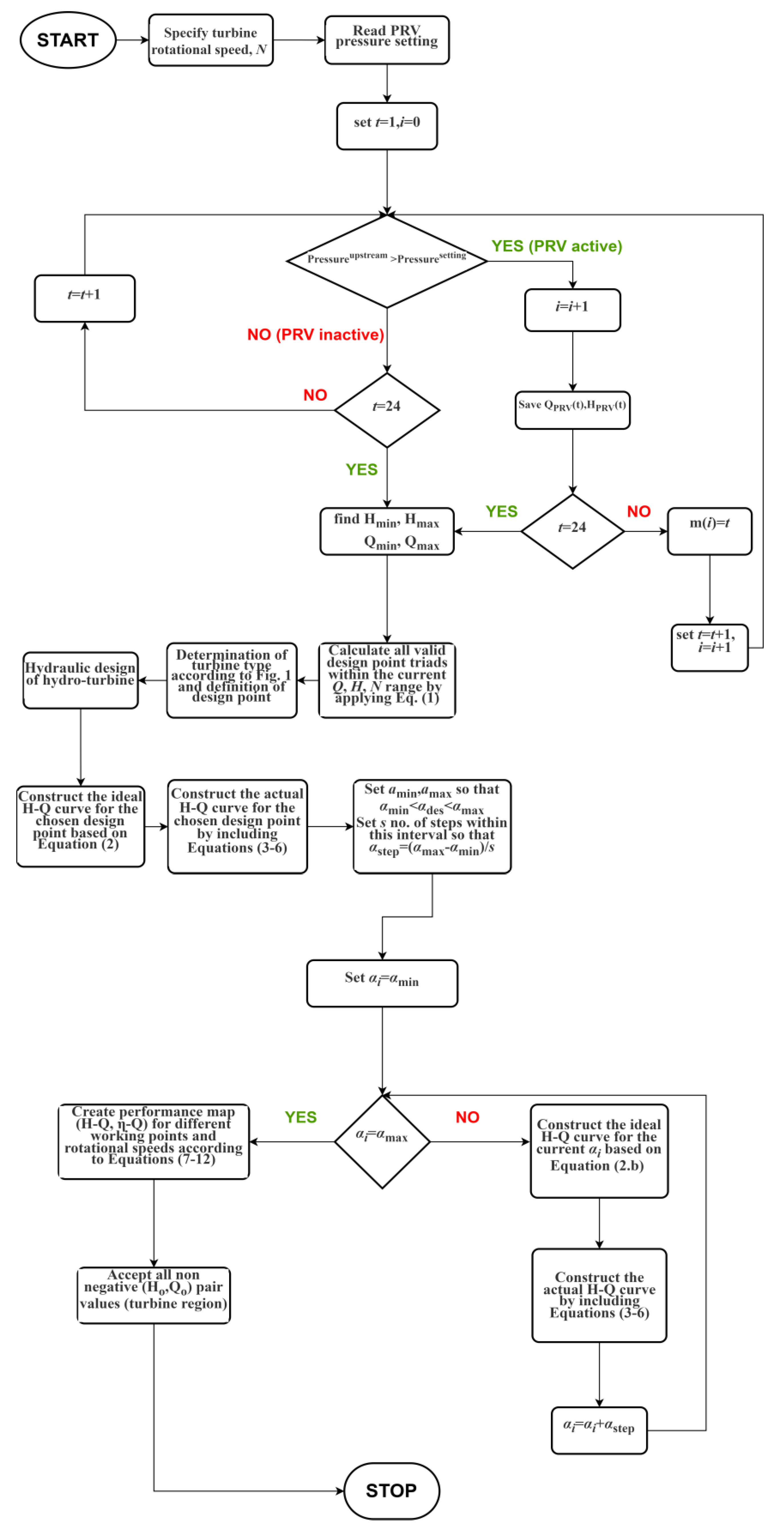
The algorithm is divided into two processes that interact with each other via the EPANET-MATLAB toolkit. The first is dedicated to the hydraulic design and performance prediction of hydro-turbines and is exclusively performed within the MATLAB environment. The second routine, which is performed within EPANET, integrates the turbine model within the WDS and launches the hydraulic simulation of the whole network. The interconnecting link between these procedures is the H–Q curves that are constructed in MATLAB and imported in EPANET, so that the turbine realistic operation via the GPV model is incorporated. The individual details and technicalities regarding each algorithmic process are displayed on the following flow charts (Figure 4 and Figure 5) and are extensively explained below.

3.2.1. Turbine Design and Performance Prediction Algorithmic Process

Initially, the turbine’s rotational speed and the pressure setting of all the PRVs that are scheduled to be replaced by turbines is requested. Then iteratively, for each time period t, the current PRV’s upstream pressure is compared with the pressure setting. If the upstream pressure is greater than the pressure setting then the PRV is active and the corresponding pipe flow along with the actual head drop (H^upstream − H^downstream) is stored. At the same time, the total number of hours i and the exact set of hours within the day m(i) that the PRV is active are stored, before the algorithm proceeds to the next time period t. If the upstream pressure is less than or equal to the pressure setting, then the PRV, and successively the GPV/turbine, is considered as inactive. In this case, the algorithm skips the current time period t and advances to the next one (t + 1). When the final time period is reached (t = 24 h), the process continues with the calculation of the flow rate and head loss profile that is achieved during the PRV’s active periods and is later requested by the GPV/turbine operation. Next, according to the current pipe flow rate and PRV’s head loss range, the methodology explained in Section 2 is applied to determine the proper dimensioning and turbine working point. This eventually leads to the construction of the actual H–Q curve for the suggested design point. This H–Q curve is also constructed for different angle values α₁, which are close to the design point value ${\alpha }_1^{des}$, by applying Equation (2b). By implementing the similarity laws around the design point, by means of Equations (7)–(11), the performance map of the hydro-turbine, i.e., H–Q and η–Q curves for different N and α₁, are created. From these curves, only the non-negative H_o–Q_o pair values are accepted (see “turbine region” in Figure 3). At this final step the process terminates, and its output is stored as a performance map and is ready to be imported to the EPANET environment.

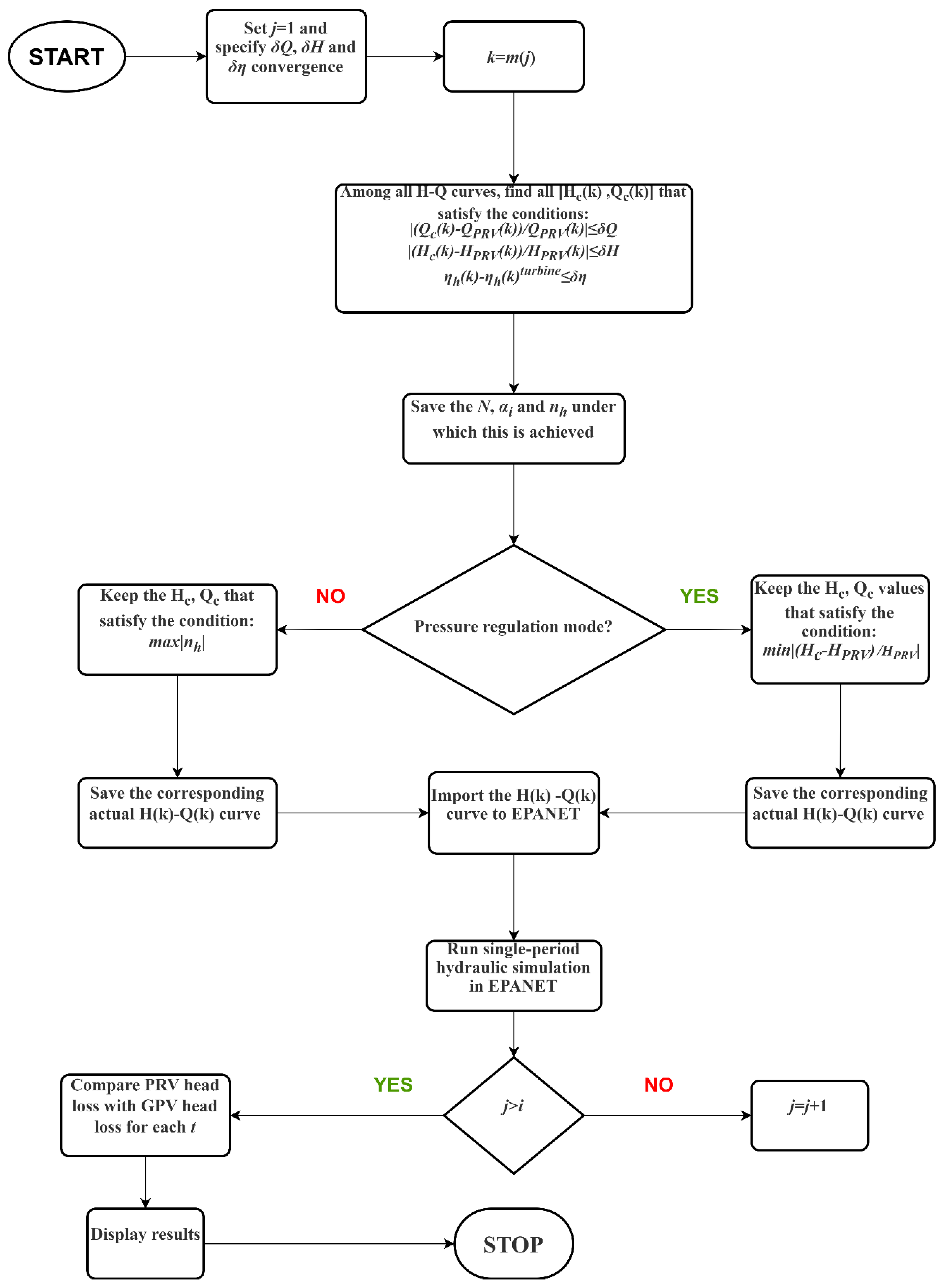
3.2.2. EPANET-MATLAB Interaction Algorithmic Process

Starting from the first active period k (first time period that GPV/turbine is active), the requested convergence of flow, head and efficiency is determined: δQ = |(Q^requested − Q^achieved)/Q^achieved|, δH = |(H^requested − H^achieved)/H^achieved|, δη = |(η^requested − η^achieved)/η^achieved|, respectively. For the given k, each H–Q curve is swept in order to trace the R number of candidate combinations {[H_c(k), Q_c(k)]¹,…, [H_c(k), Q_c(k)]^R−1, [H_c(k), Q_c(k)]^R} that approach the requested H_PRV(k), Q_PRV(k) values, under the given δQ and δH convergence value. In the meantime, the corresponding [N(k), α₁(k), η_h(k)]¹,…, [N(k), α₁(k), η_h(k)]^R−1, [N(k), α₁(k) and η_h(k)]^R values are stored. At the next step, depending on the current operating mode, the hydro-turbine can optimize its performance in two ways. It can be set to either maximize its efficiency, by operating as a power generating machine irrespective of the head loss that is achieved, or to minimize the head loss deviation by operating as a pressure regulating “device” that precisely mimics the PRV action. The δQ and δη are specified only during the “max efficiency mode” and δQ and δH during the “PRV mode”. Results where the minimum head loss deviation is achieved for H_c > H_PRV or Q_c > Q_PRV are accepted only when their percentage difference is lower than 5%. In any case, from the R number of combinations the proper H(k)–Q(k) curve is selected and then imported in EPANET’s GPV model and a single-period simulation is launched. This procedure repeats for all turbine working periods i. Before its termination, the algorithmic process provides access to all important results, e.g., head loss absolute difference between PRV and turbine action, energy produced along with the hydraulic efficiency, rotational speed, and angle α₁ variation (see Section 4).

4. Application Example

In order to demonstrate the practicality and robustness of the algorithmic process, before anything else it is required to use data drawn from a real water network of reasonable scale, that:

• Presents both branched and loop configurations;
• Consists of classic infrastructure and components, such as reservoirs, tanks, pipelines, pumps, etc., with typical sizing;
• Supplies consumers who display representative water demand requirements and demand patterns;
• Experiences high pressure in certain areas;
• Features conventional control pressure mechanisms such as PRVs.

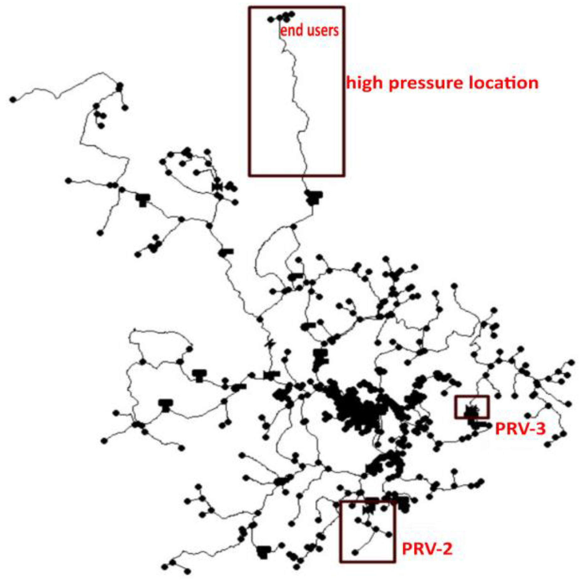
KY10 is a primarily branched network that also displays a looped configuration, as shown in Figure 6 [28]. It consists of many tanks, pumps, nodes and water pipes and provides 2.26 million gallons (8.555 thousand cubic meters) of water to its 9093 consumers daily. Along with its physical attributes there are several PRVs that regulate downstream water pressure to specific setting values. These predetermined values not only preserve the functionality of the nearby parts of the WDS, but also act beneficially for the overall network reliability. The most important characteristics and pipe data for this WDS are summarized in

Table 1. Network characteristics.

Network Characteristics	Value
Number of total pipes	1043
Number of branch pipes	473
Number of junction nodes	917
Number of reservoirs	2
Number of tanks	13
Number of pumps	13
Number of serviceable population	30,681
Ratio (Residential/total costumers)	0.92
Ratio (Residential/total water usage)	0.84
Estimated Annual Water Loss (%)	6
Water cost per 3.78 m3	6–8

and

Table 2. Pipe data.

Pipe Diameter (mm)	Total Length (km)	# of Pipes	Pipe Material for Locations
25.4	0.413	9	x
50.8	17.79	105	x
76.2	26.74	42	x
101.6	104.34	188	GPV-4 (vitrified clay)
152.4	207.49	307	PRV-2 + PRV-3 (PVC)
203.2	49.54	293	x
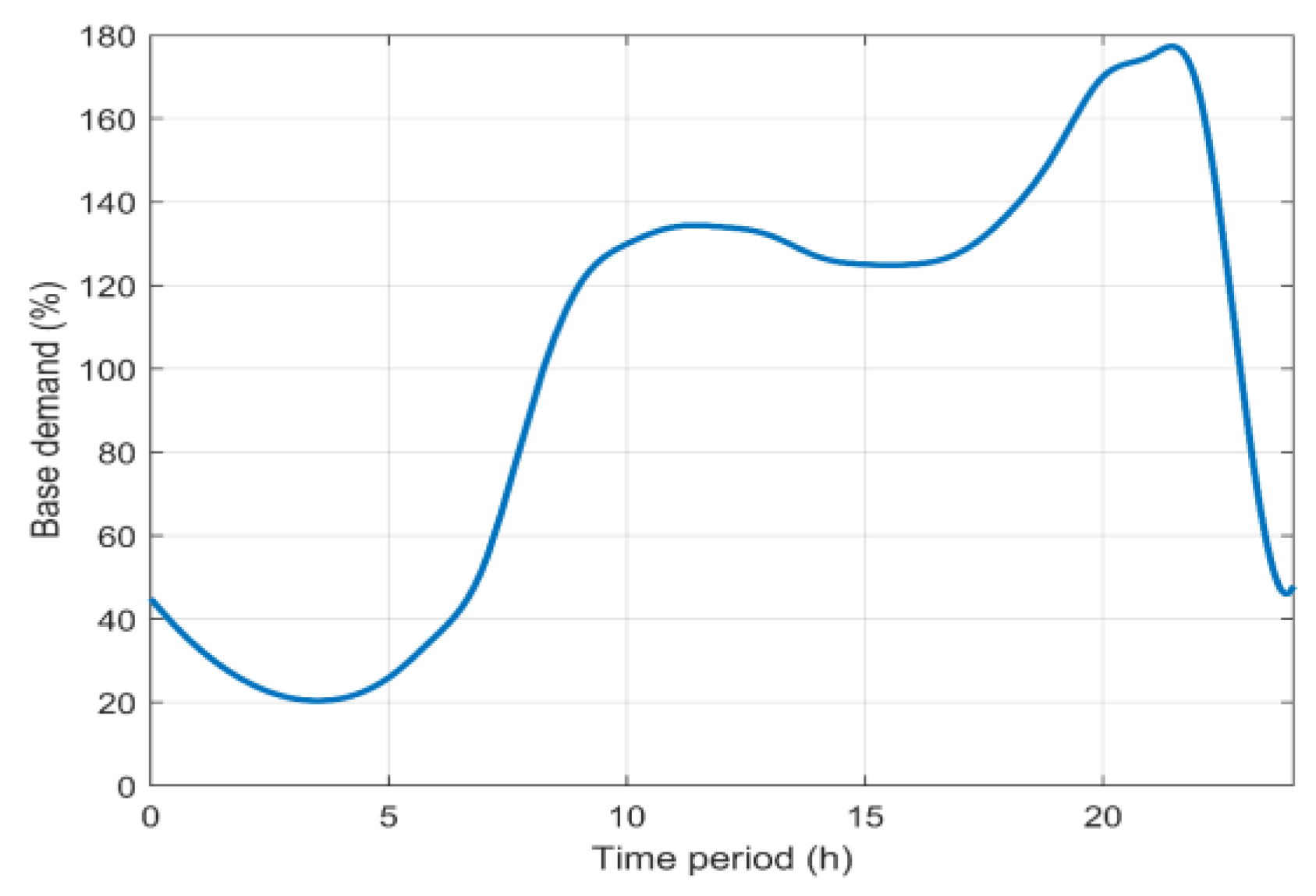
304.8	6.34	53	x

, respectively. Network pipe material is Polyethylene-PE (10%), vitrified clay (37%) and Polyvinyl chloride-PVC (53%), although all materials have been assumed to be in the beginning of their life cycle without harming the generality of the suggested methodology, since they could be adjusted to specific aging data if available. Since the simulated network consists mainly of residential consumers (92% of total users), the hourly water demand follows the pattern of the typical residential consumer, as is depicted in Figure 7.

The optimal location of hydro-turbines and PRVs in a WDS is still a subject of research [19,21,23,24]. However, in this paper we focus on a dimensioning algorithm that designs turbines operating as PRVs. Therefore, obvious network points for installing the hydro-turbines are those network pipes where PRVs are already, or should be, installed. To test the model’s credibility, it is intended to examine three different network points, as presented in Figure 6. The first two points are chosen because there are PRVs (named ‘PRV-2’ and ‘PRV-3’) already installed at these exact locations. The last network point does not currently contain a PRV, but it is chosen solely because the end users at its downstream exhibit unacceptably high water pressure values. Hence, a turbine is suggested to be installed in order to harness the excess energy that exists in the form of pressure, while regulating that pressure at an acceptable level.

4.1. PRV Replacement with Turbines

In this paper, three cases have been examined. The first two cases concern the replacement of PRV-2 and PRV-3, respectively, as shown in Figure 6. As is explained in detail in Section 3.1, before determining the turbine’s main dimensioning and design point it is mandatory to run a preparatory EPANET simulation in order to collect information about PRV operation, water flow and velocity. The Pressure Settings (in bar) of the downstream node of PRV-2 and PRV-3 are 5.51 bar and 2.75 bar, respectively. 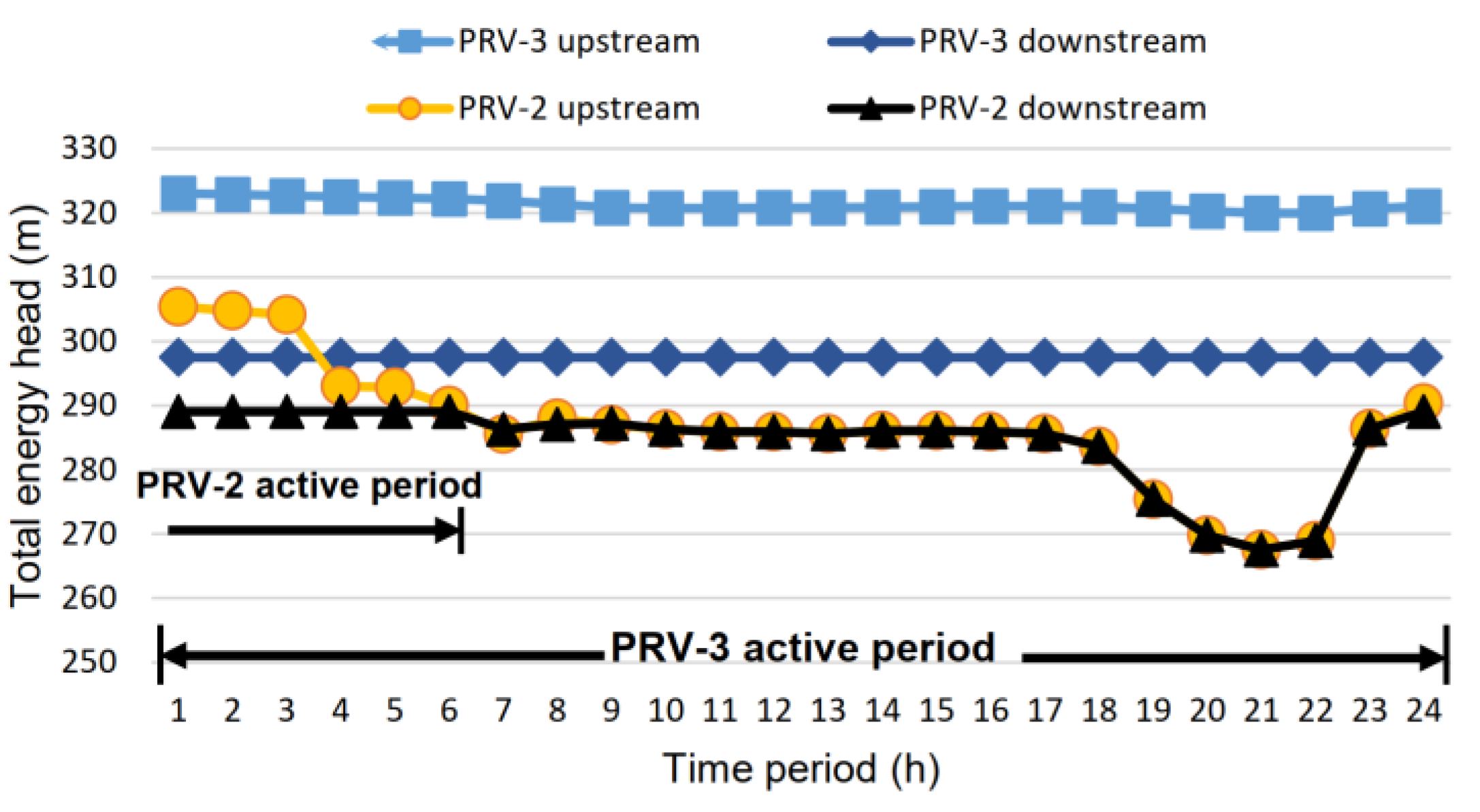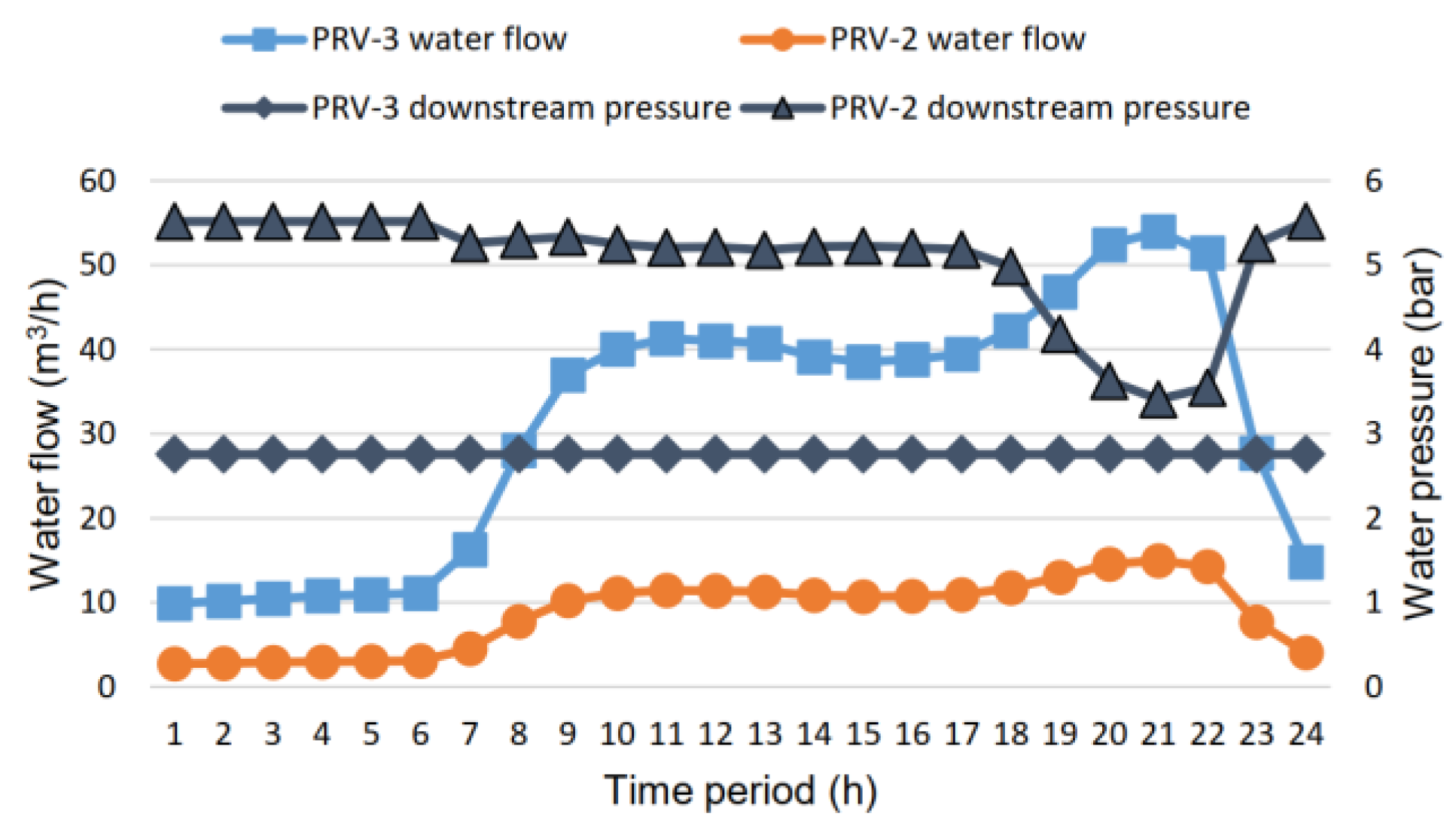Figure 8 presents the PRV-2 and PRV-3 upstream and downstream node head data, while Figure 9 contains their downstream pressure along with the flow values of the corresponding pipelines. Because of their high inlet pressure, PRV-2 is active during the first six hours and PRV-3 is active during the whole 24-h period. This means that the GPV that corresponds to PRV-2 (GPV-2 in terms of EPANET simulation model henceforth) will be designed to operate for the first 6 h, and then its status should be set to inactive while the GPV that relates to PRV-3 (GPV-3 henceforth) will be designed to fully operate during the whole day.

According to Section 3.1, the GPV-2 and GPV-3 diameters should be set to 102 mm and 152 m, respectively, so that they match the corresponding pipeline diameters. For pipelines with diameters lower than 300 mm, the water velocity, from an economical and practical standpoint, ranges near 1 m/s [53]. Hence, the values of 0.5 m/s and 1.5 m/s are being adopted as lower and upper velocity limits, respectively.

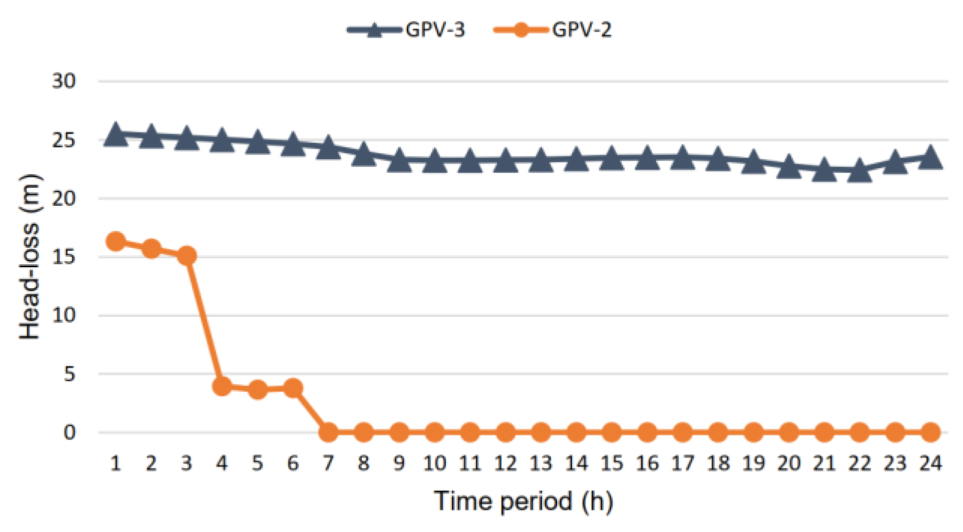
The available water flow for GPV-2 and GPV-3 is displayed in Figure 9. In particular, the flow through the pipe that feeds GPV-2 ranges between 1.48 and 1.68 m³/h, with a head loss ranging between 3 and 16 m. The flow through the pipe that feeds GPV-3 ranges between 9.72 and 54 m³/h, with a head loss ranging between 22 and 26 m. 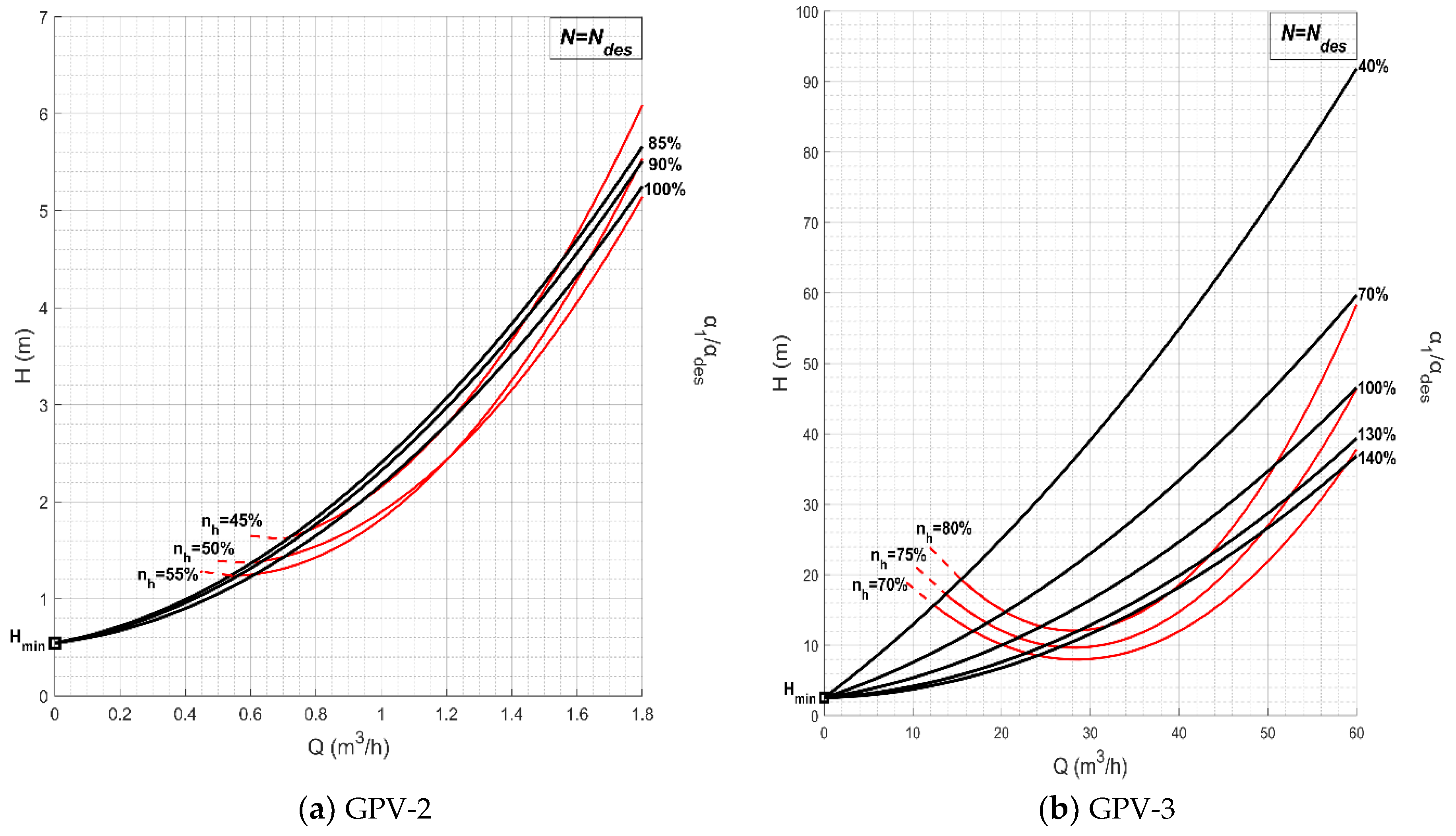The head loss requirements for GPV-2 and GPV-3 are summarized in Figure 10 by subtracting the corresponding upstream and downstream head values of Figure 8. The significant fluctuations in both flow and head indicate that the hydro-turbines are not expected to always work under design point conditions. In Figure 11, a set of characteristic H–Q curves and η–Q curves are presented for the cases of GPV-2 and GPV-3. These curves are constructed for design rotational speed N_des and values α₁ and η_h around their corresponding design point values α_des and ${\eta }_h^{des}$. Under this consideration, the H–Q curves’ starting point is calculated in Equation (14) by setting Q = 0 to Equations (2.b), (4) and (5), respectively, and deploying Equation (3):

$$H_{\min }=H_{Q=0}^{ideal}+H_{Q=0}^{losses}=H_{Q=0}^{ideal}+\delta H_{Q=0}^{friction}+\delta H_{Q=0}^{shock}=-\frac{u_2^2}{g}+{\zeta }_s·\frac{u_1^2}{2g}=\frac{1}{g}\left({\zeta }_s·\frac{u_1^2}{2}-u_2^2\right)$$

(14)

Since each of these curves is calculated for constant rotational speed and ζ_s is considered constant at the fully turbulent region (see Section 2.1), H_min has a fixed, but different, value for each GPV case. In this paper, due to the constant variation in the turbines’ operating conditions, multiple equivalent curves were constructed for different runner rotational speeds.

4.2. Turbine Placement at a Location Suffering from High Pressure without PRV Installed

In order to further demonstrate the method’s effectiveness and showcase the universality of the algorithmic process, a third network point is selected that does not accommodate a PRV. Even in well-designed WDSs there are always certain network areas and nodes that exhibit high pressure head values, e.g., network areas with high topographic gradients that at the same time are not equipped with a PRV [20]. These cases constitute an opportunity to assess the effect of a possible hydro-turbine installation instead of a PRV.

However, not all nodes with excess energy should be considered as candidate points for turbine installation. Depending on network layout and topographic features, the excess pressure that appears in various nodes is often required to ensure a minimum pressure in other nodes or areas and secure a service quality that is imposed at local–national level by the regulators [20]. Especially in networks with dense looping characteristics, it is even harder to determine whether the excess energy in pipes and nodes is “free” to use or mandatory for preserving network stability.

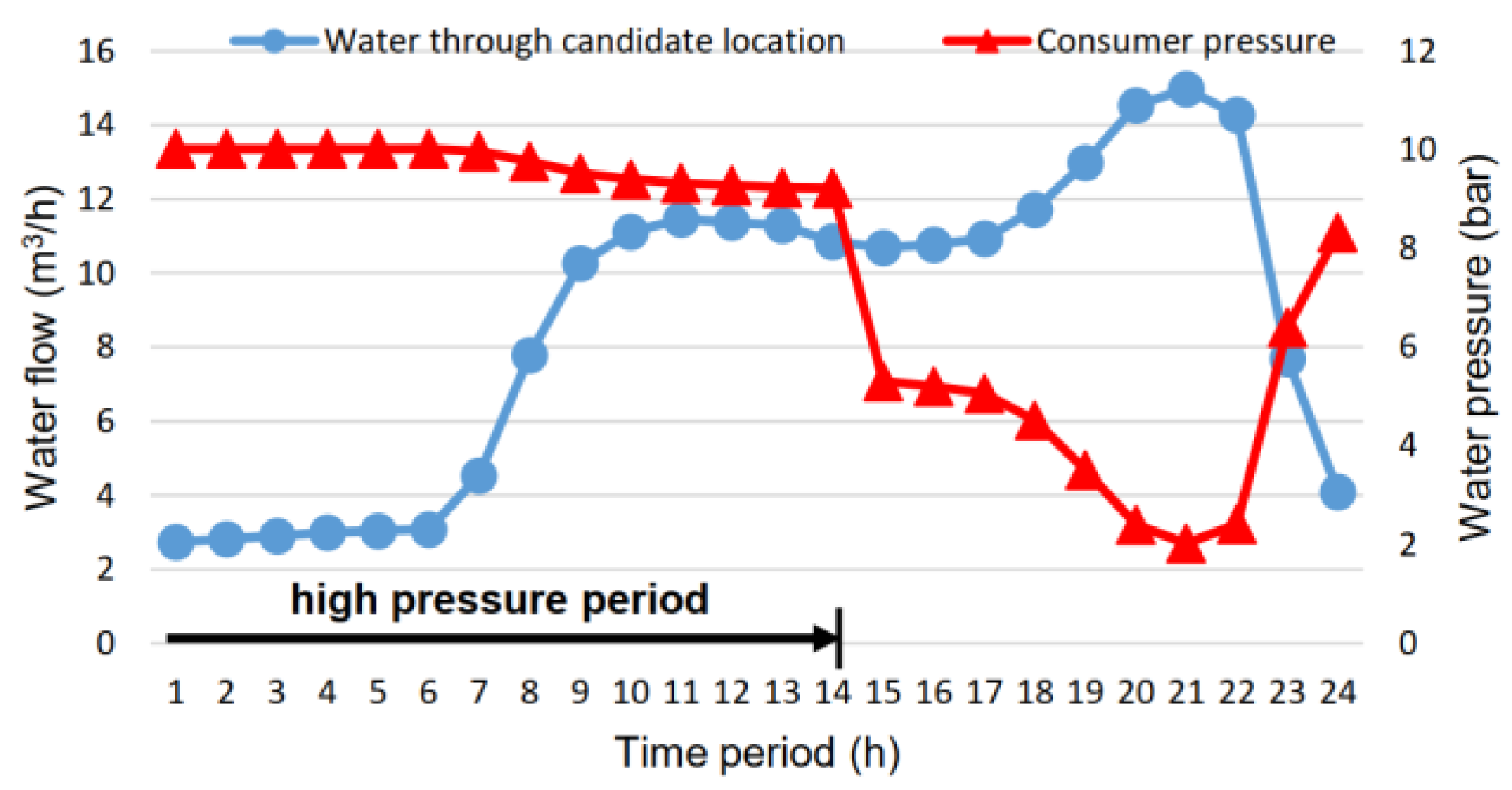
Just like GPV-2 and GPV-3, a preparatory EPANET analysis was executed to pinpoint an appropriate network location that suffers from high water pressure without a PRV currently installed. Taking this into consideration, an end-pipe network node in a branch configuration that exhibits an excessive pressure head is examined. Due to this branched layout, the impact of a GPV can be well assessed beforehand to retain the area’s former functionality. 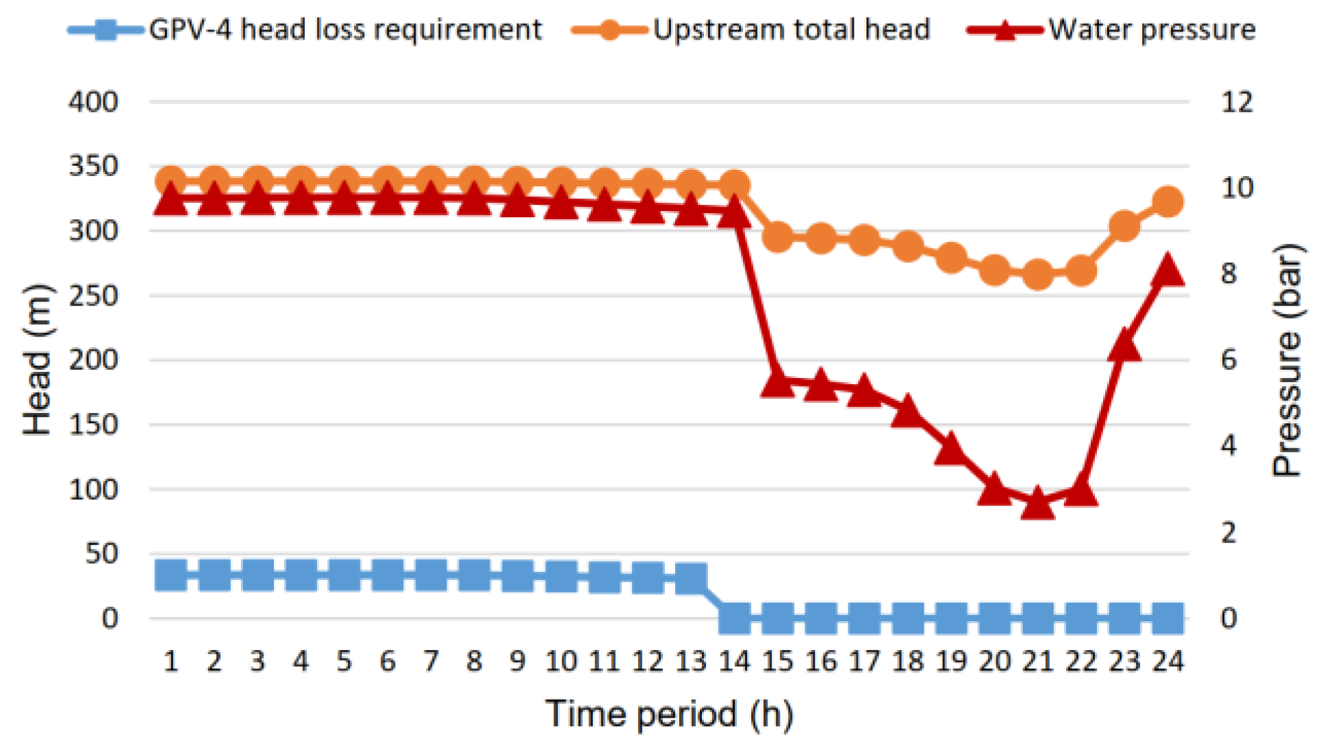This network area is displayed in Figure 6, while the pipe flow and nodal data are presented in Figure 12 and Figure 13, respectively. 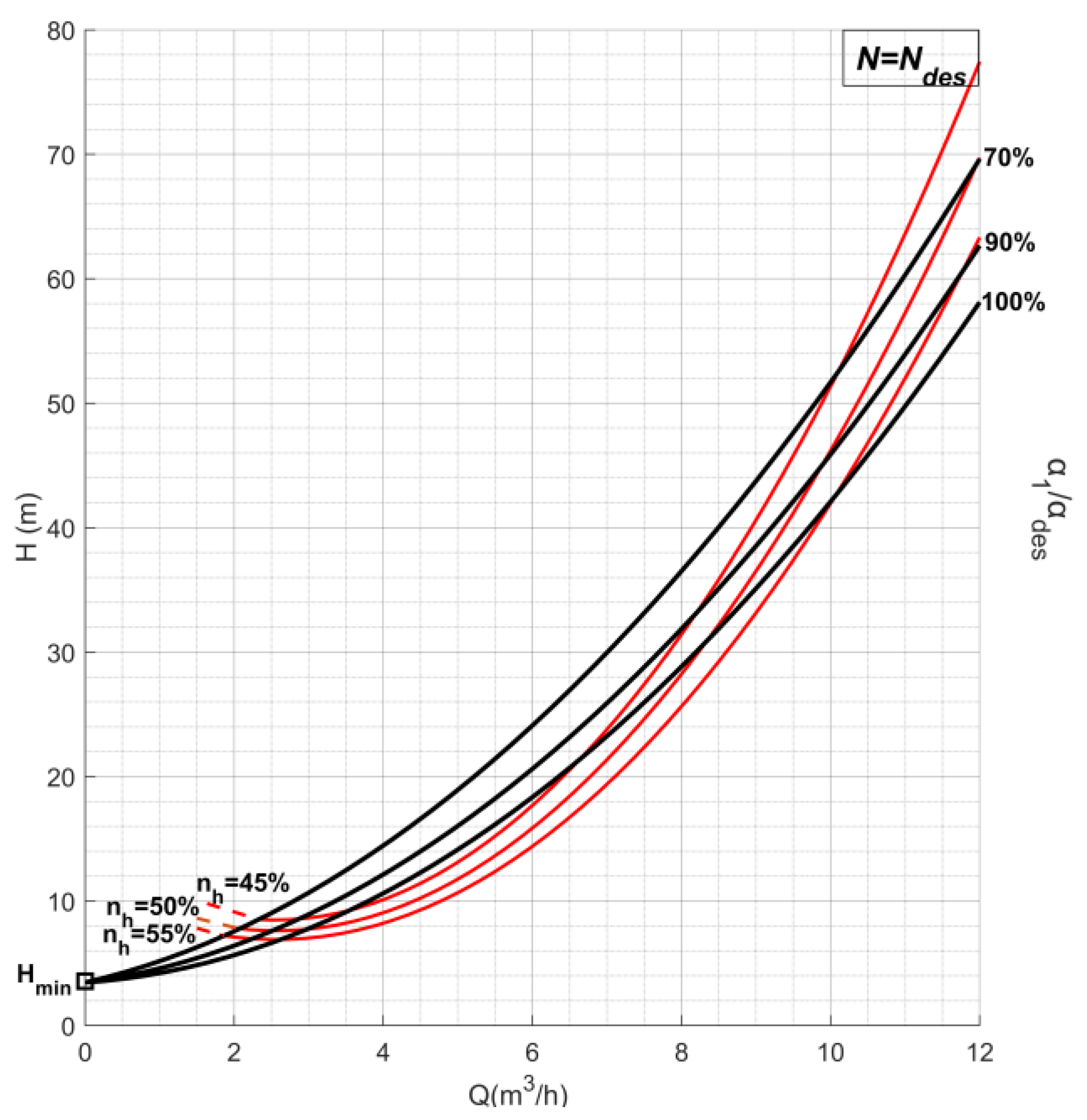The junction water pressure for the first 13 time periods (t = 1–14) ranges from 9.4 to 10 bar, which is considered extreme for the consumer side. At the same time, a minimum pressure threshold needs to be secured and only the excess pressure should be exploited for energy production purposes. In order to ensure that the particular network area is not negatively affected by the proposed hydro-turbine installation, the exact pressure threshold value should be investigated by a separate study, which is considered beyond the scope of this work. To be on the safe side, it is reasonable to assume a pressure threshold of 6 bar at the GPV outlet. By accomplishing a regulation of pressure at a lower level the smooth network operation and service quality is maintained, but also reduced pipe head losses are achieved. For this reason, the installation of a suitable hydro-turbine (GPV-4 henceforth) is considered. The head loss that must be accomplished by GPV-4 for each time period, in order to maintain the pressure threshold, is presented in Figure 13. The corresponding characteristic η–H–Q curve for constant speed N_des and inlet angles α₁ and efficiency values n_h around the design point, is displayed in Figure 14.

4.3. Results and Discussion

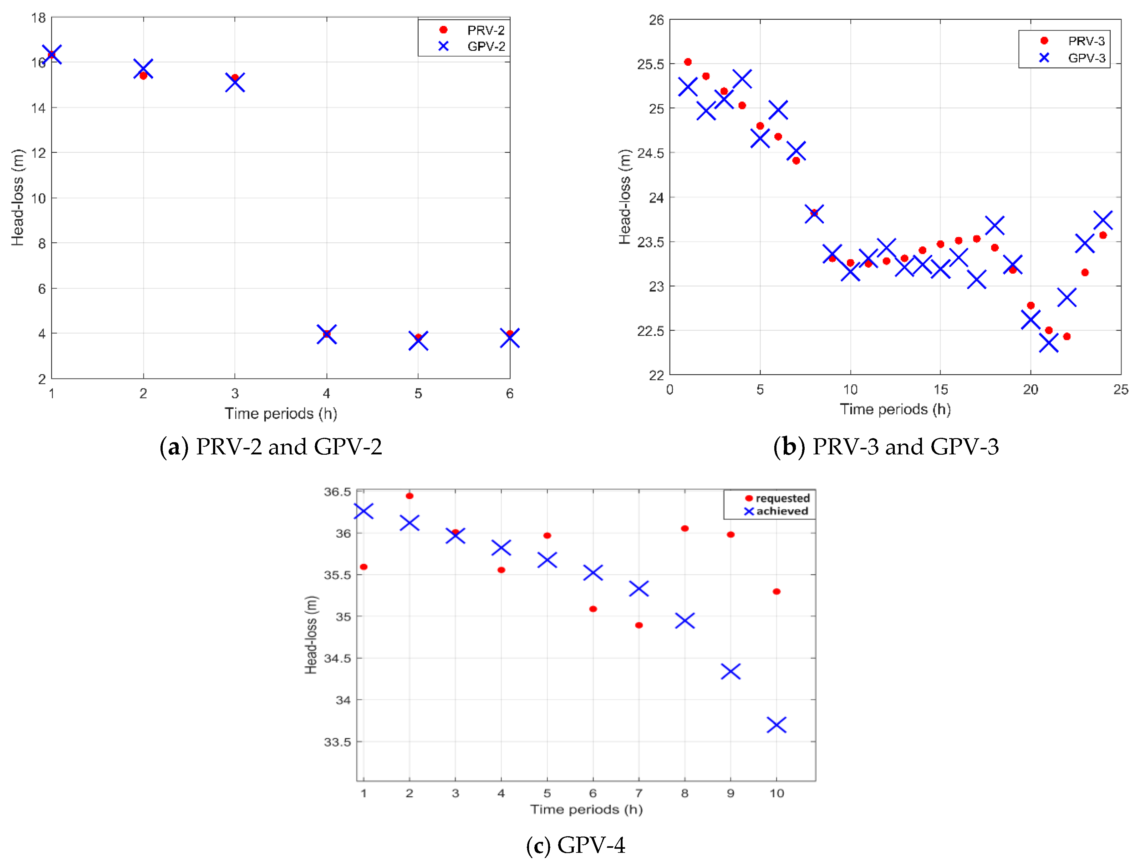
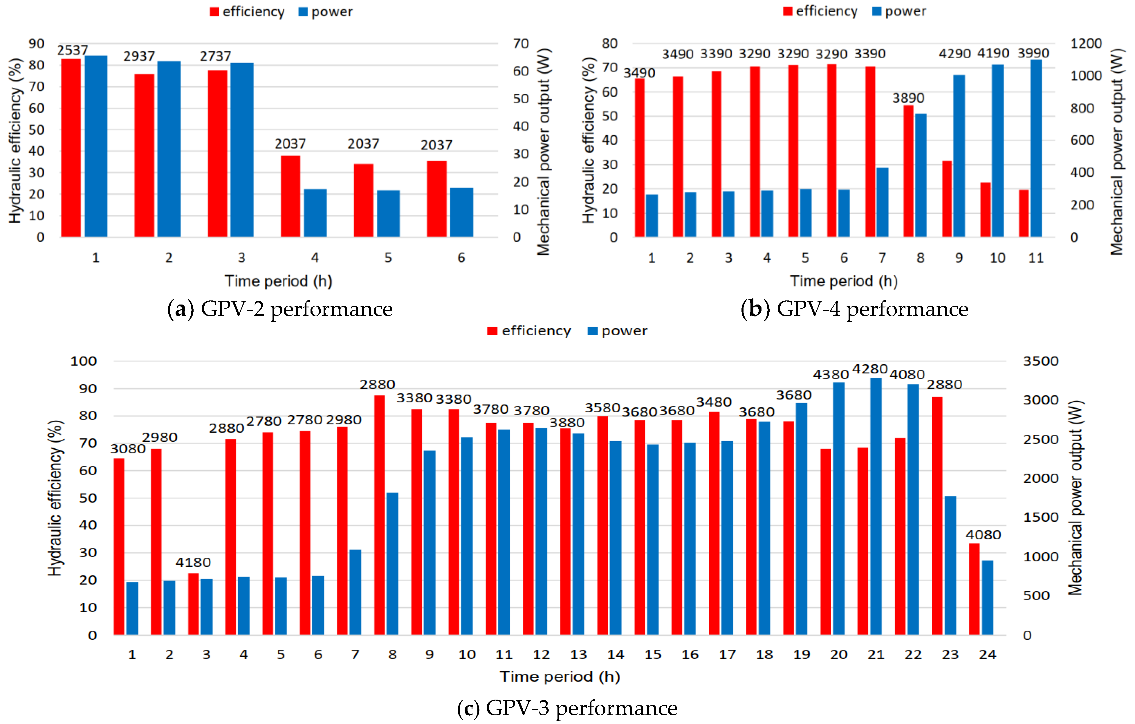
In Figure 15 the localized head loss that was imposed by the PRVs and the one that is achieved by the replacement with hydro-turbines via the GPV model are compared. Figure 16 provides access to the mechanical power output (P), hydraulic efficiency (η_h) and the rotational speed (N) at which the requested head loss values are accomplished by the turbine. Each bar in these graphs corresponds to the time periods during which the PRVs were active (i.e., downstream water pressure is above the defined PRV setting) and therefore the time periods during which the hydro turbine is requested to operate.

According to Figure 15a,b, the absolute pressure deviation between the PRVs and GPVs operation at any instance does not exceed the value of 2%, while for 70% of time periods it is lower than 1%. This small error ultimately allows the utilization of the available head at its totality and signifies a large improvement when compared to other published researches using turbines [17] or PATs [10,54]. It is worth mentioning that when the placement and setting of PRVs within the WDS is optimized with the aim of water leakage minimization through pressure control, such high accuracy in downstream pressure regulation ensures that the substitute turbine also minimizes water losses. 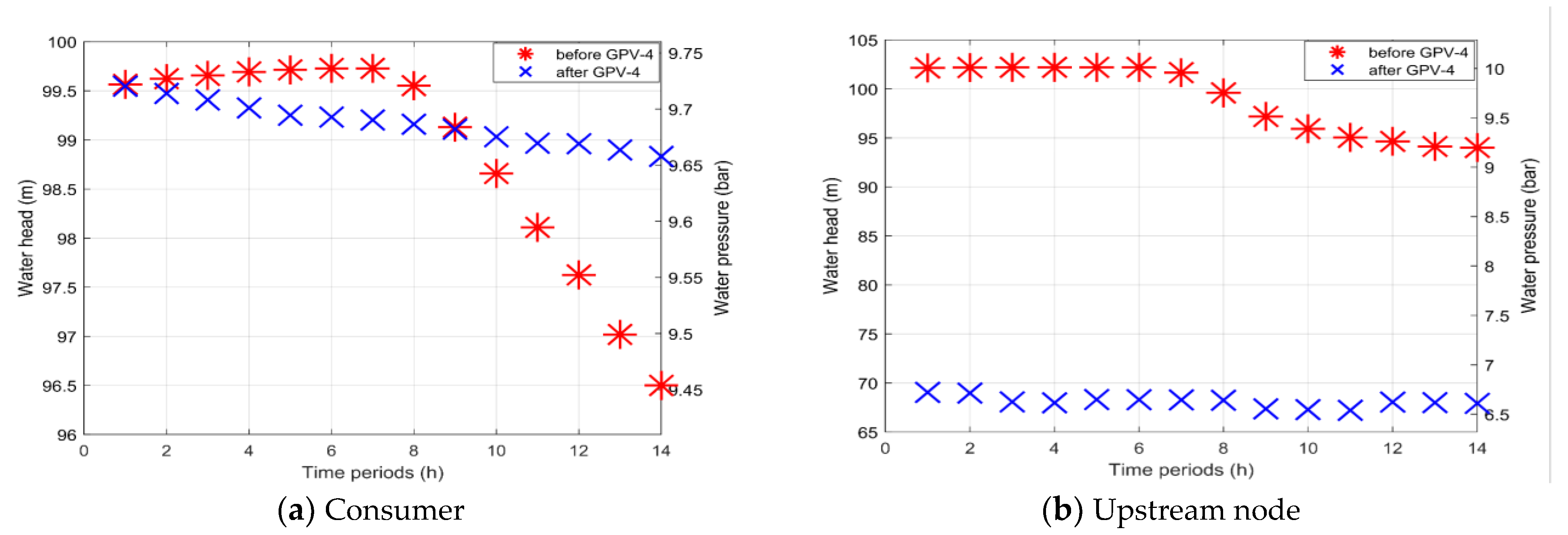At the location suffering from high pressure without PRV currently installed, the hydro-turbine managed to keep a very narrow gap between the required and achieved head loss, as shown in Figure 15c. In this case, the absolute pressure deviation between the target pressure and the one achieved by turbine’s operation ranges between 7% and 11%. At the same time, the turbine operation did not only disrupt or unbalance the upstream node conditions, but also retained the downstream-consumer pressure to reasonable and secure values (Figure 17) while simultaneously producing energy. For each case, all the important design and operational data and properties of the proposed hydro-turbines are presented in

Table 3. Important operational and design parameters.

Design Point Data.	GPV-2	GPV-3	GPV-4
volumetric flow rate, Q (m3/h) head, H (m) rotational speed, N (rpm)	1.58	36	6.84
	2.2	18.5	13.4
	1190	2410	1950
specific speed, nq hydraulic efficiency, ηh (%)	14	27	12
	52	87	55
Number of blades guide vane opening angle, α1 (°) inlet diameter, D1 (mm) outlet diameter, D2 (mm)	6	6	6
	4.85	10.3	3.8
	102	152	152
	34.7	66.4	50
D2/D1 ratio mean efficiency, ηmean (%)	0.34	0.43	0.33
	62	72	50

. It is worth noticing that compared to the nominal design point efficiency η_h that each hydro-turbine was originally designed for, the mean efficiency η_mean that derives from all time periods does not deviate significantly. For both GPV-2 and GPV-3 cases, η_mean is higher than the efficiency values (30–60%) that are typically encountered in micro sites, as is suggested by [18,55]. Especially for the GPV-3 case, the resultant efficiency and power production are considerably greater than PAT systems operating in similar flow rate conditions [10]. For GPV-2 the resultant mean efficiency value is larger than the design efficiency since the corresponding turbine, for the first half of its working period (t = 1–3), operates at flow rate, head and rotational speed values that are far from the selected design point. At these operating conditions the resultant hydraulic efficiency is significantly larger (70–80%) than its design point value (52%), which is approximately achieved during the second half of its working period (t = 4–6).

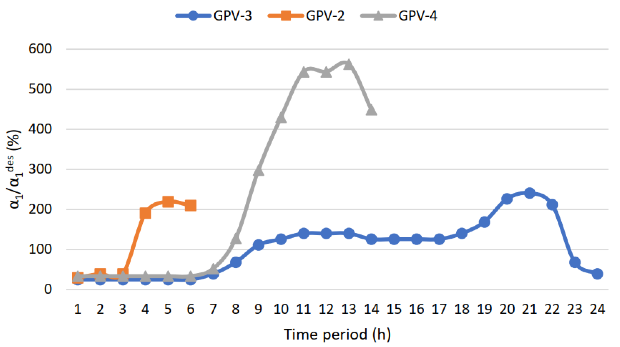
As it can be noticed from Figure 16, GPV-2, GPV-3 and GPV-4 produce an average mechanical output power of 40W, 2kW and 777W, respectively. A considerable amount of “green” energy can be produced that otherwise would be dissipated by the PRVs. In particular, during the 24-h working period approximately 48 kWh were produced by the GPV-3, while 244Wh and 9 kWh were produced by GPV-2 and GPV-4 during their 6- and 14-h working periods, respectively. It is worth noticing that only in a few time periods were the hydro-turbines forced to work under low efficiency in order to achieve their main task, i.e., to deliver a specific pressure to the outlet. The significant variance between the hourly energy production between locations is solely explained by the great difference between volumetric flow rates (see Figure 9 and Figure 12). Radial hydro-turbines tend to work less efficiently in low volumetric flow rates, such as the ones supplied to GPV-2 and GPV-4. Finally, in Figure 18 the variation in angle α₁ with respect to the original design point value α_des is displayed for each time period and GPV. It is clear that for the GPV-3 case the selected design point is considered adequate, since the α₁ variation is most of the time close to the design value, and thus close to BEP. Conversely, for the GPV-2 case, the energy potential is so low that any related improvement in design and performance is considered unprofitable.

The efficiency of typical 4 pole electrical generators is calculated according to the IEC Standard for efficiency classes [56]. Since GPV-2 produces an average mechanical output power of 40 W, it is reasonable to assume an efficiency between 0.5 and 0.6 (IE3 class and above). Therefore, the daily electrical energy output will range between 0.12 and 0.144 kWh. Similarly, for GPV-3 and GPV-4 that produce an average mechanical output power of 2 kW and 777 W, respectively, the final efficiency will range between 0.85–0.9 and 0.82–0.85, thus leading to a total power output range between (40.8–43.2) kWh and (8.28–8.56) kWh, respectively.

5. Conclusions

The paper provided a step-by-step algorithmic methodology for replacing the existing PRVs of a WDS with hydroelectric turbines. Among other energy recovery machines (turbines or PATs), the Francis turbines were selected mainly due to their suitability for PRV replacement, i.e., they accomplish the same downstream pressure under varying operating conditions, with corresponding high efficiency.

More specifically, the proper geometry and suitable design point of a hydro-turbine that manages to achieve the same exit pressure as the downstream pressure output of a PRV were tested in a typical network. For this purpose, an external MATLAB algorithm was developed, and with the use of EPANET-MATLAB-toolkit it was demonstrated that a hydro-turbine’s operation replicates the function of a PRV and converts energy losses to electricity. The algorithm has been tested on three locations of the simulated WDS, each with different hydraulic conditions. It suggested appropriate turbine designs for each location, which managed to maintain a consistent pressure set point at their exit despite the wide range of the required pressure drops and the available water flow at their inlet. The constant shifting to different H–Q and η–Q curves by the accurate adjustment of the incidence angle of the blades at inlet that leads to a corresponding change in the rotational speed, has proven to be a very efficient and reliable technique in terms of achieving the desirable pressure drop at hydro-turbine’s exit.

In this research, a methodology for the design of hydro-turbines is developed so that they can precisely replicate PRV operation with energy production efficiency, despite the big flow rate and head variations in WDSs. Many researchers investigate the economic benefit of replacing PRVs with recovery machines, such as PATs, just from the perspective of dissipated energy. However, for the first time, the actual deviation between PRV and turbine operation in terms of downstream pressure is provided. This research also provides guidelines to create “active” PRV equivalents, which not only effectively contribute to the network’s water management, but also exploit the otherwise dissipated energy with considerable efficiency. Suggested turbine designs manage to maximize the exploitable head (H^achieved) by matching it with the total available head that is requested by the PRV (H^requested) with low errors (2% maximum). At the expense of computational time, these errors could potentially be further improved if a smaller step during consecutive values of α₁ and N is used. This work proves that a Francis turbine in a WDS can handle extreme variations in flow rate and head by fully exploiting the available head, with high efficiency in a wide range of working points and not just close to the BEP. The average efficiency displayed during the PRV replacement scenarios (GPV-2 and GPV-3) is superior to efficiencies presented in relevant research for micro sites.

Thus, the suggested methodology can be applied in real WDS as a preliminary procedure performed by the water network manager for the determination of the appropriate turbine type and size, along with its pressure regulation potential and power output. To this end, it can be used as a reference for developing pipeline hydro-turbines and assess their long term economical and practical viability compared to the retention of PRVs. The proposed method has been tested on a specific network, but provides a general methodology that can be easily adapted and extended to other network configurations with different PRV sizes and settings. The applicability of the proposed methodology, however, is not limited only to Francis turbines. The best turbine type and dimensioning adapts to the pipe flow rate and the head variations demanded by the PRV operation. In other networks with higher flow rates or/and less varying PRV head loss demands, other turbine types, reaction turbines such as Deriaz or Kaplan, may prove to be more suitable.

It was proven that in locations with significant energy potential, i.e., high flow rate and head (e.g., GPV-3 case), the replacement of the existing PRV could be economically justified because the resultant hydropower generation surpasses the investment costs (purchase, installation, maintenance) of the turbine. Conversely, in scenarios with low flow rate (e.g., GPV-2 case), even though the turbine operation accomplishes the same head loss with the PRV, the negligible energy production cannot compensate for the high installation cost. In such extreme cases even the installation of a cheap PAT system would be proven unprofitable, and thus, maintaining the existing PRV represents the most convenient and viable option.

Moreover, a complex WDS contains various promising locations and candidate network points where the installation of a hydro-turbine is not only considered to be a feasible perspective, but also proven extremely valuable for both pressure management and clean energy production. These locations can range from network points where a PRV is already installed (cases 1,2) to “arbitrary” network points whose profile displays appealing features (case 3) such as low elevation, high pressure, high water flow, or ideally, a combination of the former. The economic and environmental benefits that arise from the use of micro hydro-turbines in both pressure management and energy production are summarized below:

In terms of pressure management:

• From a WDS standpoint, the replacement of a PRV with a suitable hydro-turbine does not affect the former network operational conditions, i.e., flow and pressure, or disrupt its functionality; therefore, it does not add any operating challenges to the actual network. The limitation of the excessive pressure head in certain regions can only work beneficially for the network as it leads to the restriction of water hammer occurrences that are often considered as the main pipeline failure cause;
• From a consumer standpoint, the service level is preserved when replacing a PRV with a hydro-turbine, or even upgraded in cases where a PRV is absent and a hydro-turbine is purposefully installed in a certain consumer area, in order to secure that this area will witness normative water pressure values. Ιn this latter case, the resulting pressure drop can also lead to scaled-down pipeline head losses, i.e., less total energy losses and reduced pipeline stress.

In terms of energy production, the implementation of micro-hydropower within the WDS unlocks the possibility of urban and renewable power generation that:

• is fed the electrical grid with predictable and nearly constant amount of power;
• is consumed locally;
• does not create any visual or audible nuisance.

The main limitation of this work is that it utterly relies on the network PRV locations and their current pressure setting point for assessing the hydro-turbine size and performance (GPV-2 and GPV-3 case). In real WDSs, PRVs installation location and pressure setting are usually selected with the objective of securing network operating constrains and preventing extreme pressure in the consumer side. Thus, there exist time periods where the downstream pressure could be potentially reduced for water savings maximization purposes. Consequently, maximum power production or water savings are not always guaranteed unless the PRVs placement within the WDS has been already optimized and selected with the aim of maximizing the available energy at their inlet, or PRVs can change their pressure setting in real time. This is confirmed for the PRV-2 case, as it has minimal energy recovery potential. Its placement was clearly destined for pressure containment and not energy production. Finally, the results of the GPV-4 case have been recorded assuming a “safe” pressure threshold of 6 bar. The actual optimal pressure that achieves maximum power output and ensures sufficient service level to the certain area has not been determined.

It is the target of future work to create a common model for the urban hydraulic and electric systems. Such a model is expected to accommodate the objective of maximizing absorbed power from the WDS, considering the constraints imposed by both the hydraulic system (e.g., minimum acceptable pressure at customer nodes) and the power system (e.g., voltage levels within acceptable range). The link between the two systems will be the micro-hydro turbine model presented here. Finally, the hydro-turbine installation process could be improved by pre-processing the network data as a whole and ending up with an algorithm that pinpoints the optimal network points that represent promising cases in terms of pressure regulation capability and energy generation potential, or a combination of both. This revised algorithm should be able to decide between the optimal choice of hydro-turbines installation position, their type, number and design-working point depending on the current demands of the interconnected electrical and hydraulic network. In any case, along with pressure management a WDS should be envisaged as a renewable, predictable, silent and invisible energy source that can be locally harnessed in urban areas.