Integrated Smart Management in WDN: Methodology and Application

Abstract

Urbanization and population growth have been responsible for a significant increase in consumption of water and energy at a global scale. A careful management of water resource and infrastructures is crucial for Energy Transition, as well as for achieving a sustainable efficiency of these systems. High pressure values along with the ageing of the systems contribute to high leakage levels of Water Distribution Networks (WDN). The simultaneous control of excess pressure and containment of water losses are mainly performed by using Pressure Reducing Valves (PRVs) in WDN, which dissipate the surplus of hydraulic energy. Instead of being dissipated, energy can be recovered by the transformation of the excess pressure into electrical energy with the use of Pump as Turbines (PAT), which results in an increased reliability, reduction of cost and an overall improvement in the efficiency of WDN. The work aims on presenting an integrated efficiency management methodology in terms of Effectiveness (E), capability (${\eta }_p^i$), reliability (${\mu }_p^i$) and sustainability (${\chi }_p^i$) with values between 47 to 98%, also associated with the pressure and leakage management, and energy recovery. This research presents a modelling of a real WDN of a District Metering Areas (DMA) of Beloura endowed with seasonal consumption variability to better show its applicability. Additionally, an economic analysis to assess the solution’s feasibility is presented concluding an annual energy recovered of 9.8 MWh and a saving of about 30% of water leakage, which correspond, in the analyzed case study, to about 3523 m³. The payback period found is around 9 or 12 years, for only one PAT or two different PATs installed, due to the small available energy of the analyzed case study. Acknowledging the synergy between water and energy efficiency and taking advantage of these integrated smart management methodology exemplification, it resulted in more efficient systems to achieve both effectiveness solutions, digital and energy transition in the water sector.

1. Introduction

Water resources have a very crucial role in achieving the economic growth and environmental sustainability at a global scale. However, the management of water has never been a priority for the governments nor of importance in the opinion of public.

Since the beginning of the twentieth century, there has been an exponential rise in the world population. Furthermore, increased human life expectancy has led to intense industrialization and urbanization [1,2]. Such a growth in population and urbanization has been resulting in increasingly high water demand, whose utilization is not efficiently managed and this represents the main cause of water crisis. Moreover, it has expected that the population will increase up to 10 billion in 2050, which will reflect on an intensive use of the water resource [3,4].

Water Supply Systems (WSS) are vital in the livelihood of mankind. Nonetheless, large number of countries do not possess water infrastructures and some have substantial losses [5,6]. Moreover, the Governments do not take measures for WSSs due to economic crisis, hence the fundings are low [7]. In this regard, supplying water at affordable price without affecting the quality represents the challenge in modern WSS [8].

With reference to WSSs in Portugal, until 1990 the water management was very inefficienct, leading to system failures and degradation of infrastructures [9]. Nonetheless, nowadays there is a division in water supply and wastewater, and it is considered as a public service, of structural character, which is essential for human well-being.

In water sector, there have been continuous efforts in the promotion of water policies, by endorsing efficiency and green growth, inclining towards the improvement of the environment. Nowadays it is estimated that 99% of public water is safe, which is a significant achievement considering that this value amounted to 50% in 1993. However, water leakages in WDNs still represent a crucial issue, amounting to more than 30% on average. The PENSAAR 2020 report presents the issues related to WSS and awareness of the government which needs to be followed by all water authorities and municipalities [10].

Even though there is sufficient water to fulfil people’s needs, it is imperative to bring a change in the way the water resource is used, shared and managed [1]. Drinking water supply aggregates catchment, treatment, elevation, transportation, storage, distribution and consumption of the water resource. A great advantage of hydraulic potential can be seized in storage and distribution, which, hence, become very crucial processes. In this regard, water management authorities use energy efficiency and sustainability as performance indicators. The assessment of these parameters are performed in order to quantify the risk associated with water distribution [11]. The boundaries in water pipe systems are established by District Metering Areas (DMA) to monitor and decrease the water leakage. The DMA size is dependent on several factors, such as the topography and pipe density in networks, as well as the financial capacity of the water authorities. DMA implementation allows for a contraction of intricacy in WDN management, based on the evaluation of water consumption patterns, water and pressure monitoring, valve and tank control along with the billing information of client. This is the major action developed by authorities in the scope of water systems [11].

The main challenge for the water authorities and stakeholders is represented by the reduction of water losses, since these represent a waste of money and resource. It is reported that, rather than in larger distribution pipes, real water losses often occur in high-density pipe networks, in particular within the small end-user branches [12]. However, according to [13], most of water volume is lost in distribution pipes. In this regard, reduction of pressure is crucial to contain the amount of leaked water [14]. Efficient devices for leakage control are pressure reducing valves (PRVs), which dissipate the excess energy, keeping the pressure at desirable value [15,16,17]. However, recent studies focused on the replacement of PRVs with pumps as turbines (PATs). Microscale level energy can be, indeed, generated by PATs, which convert the surplus pressure in electrical energy [18]. However, PRVs and PATs have similar behavior in steady-state conditions, even though a difference in the peaks and wave propagation can be seen in their dynamic response in transient conditions [16,17,18], PATs being dynamically better. Compared to traditional turbines, PATs result in many advantages, such as low maintenance, repairing and acquisition costs, as well as very low environmental impact. However, a careful selection is required in order to get the best outcome in terms of system efficiency [18]. Indeed, in WDNs the strong fluctuations of flow and head patterns may lead to a decreased energy production, thus, resulting in negative economic impacts. Moreover, due to the rigid geometric configuration of volute case and impeller, PATs do not offer possibility for flow regulation, forbidding the operation at the best efficiency whenever there is a change of flow [4,19]. In spite of its disadvantages, PATs contribute to a sustainable development of water systems as they reduce the dependency on external sources of power and increase the energy efficiency of these systems [17,20].

This research paper aims to propose an integrated smart management methodology, as a reliable tool for water sector managers to improve the energy efficiency of water networks. The next sections are organized as follows:

-

Section 2 presents the fundamentals, the methodological approach and the model development;

-

Section 3 presents the description of the case study and the characterization of the analyzed system in terms of water consumption. Moreover, different hydropower solutions are considered and compared in terms of leakage reduction and energy recovery. Finally, an economic analysis is carried out in order to assess the viability of the proposed solutions;

-

Section 4 presents the conclusive remarks of the proposed work.

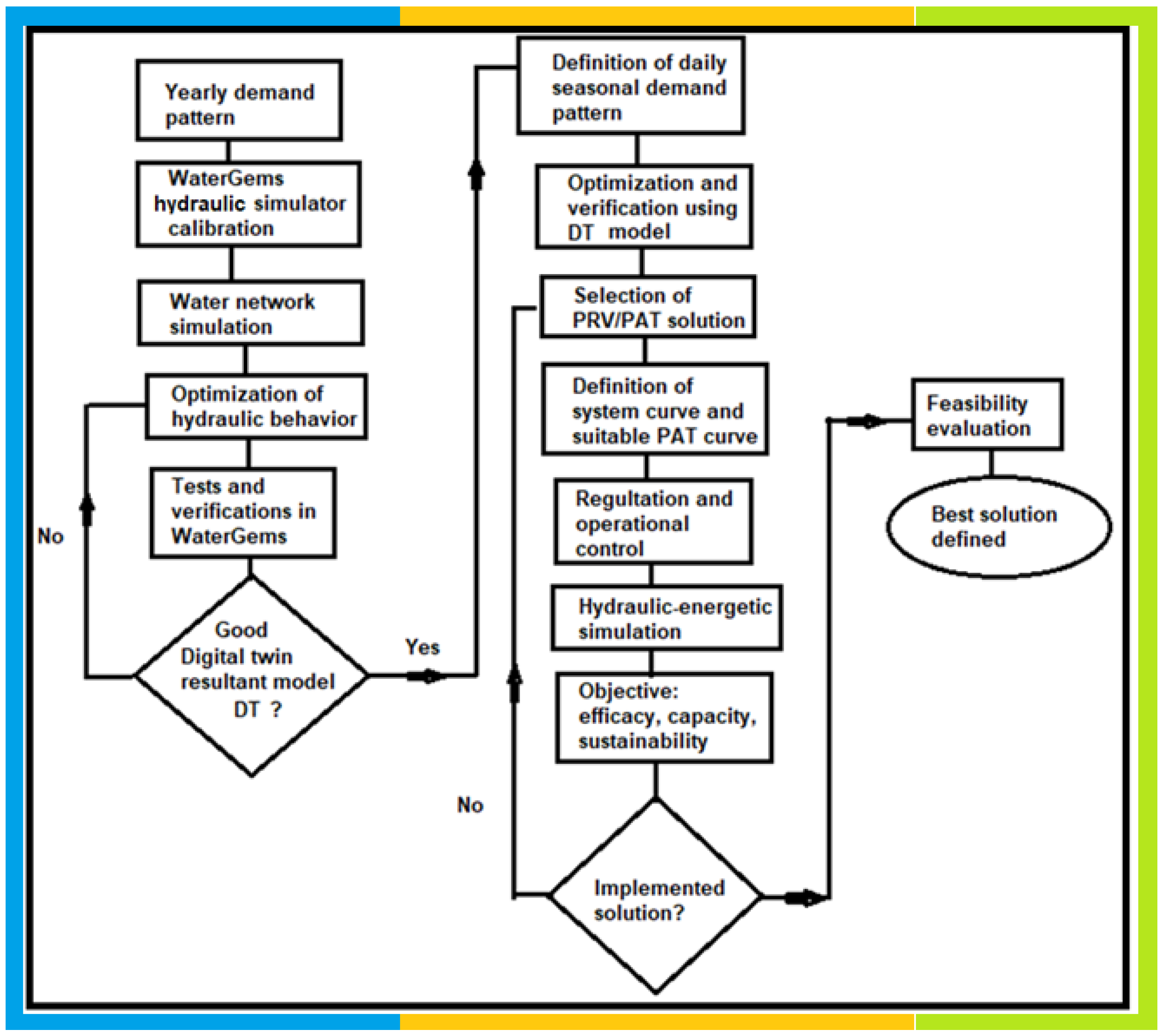
2. Materials and Methods

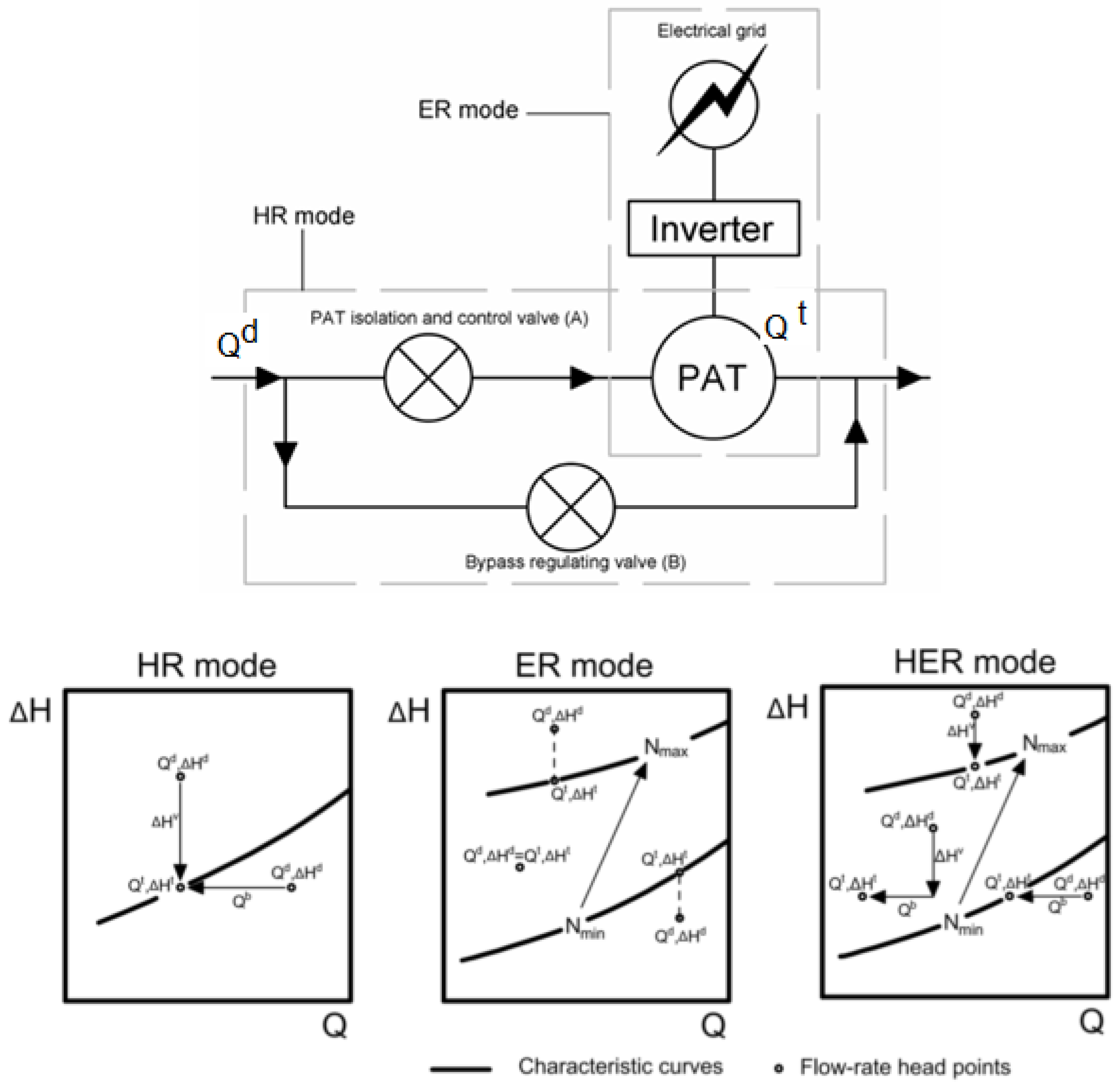
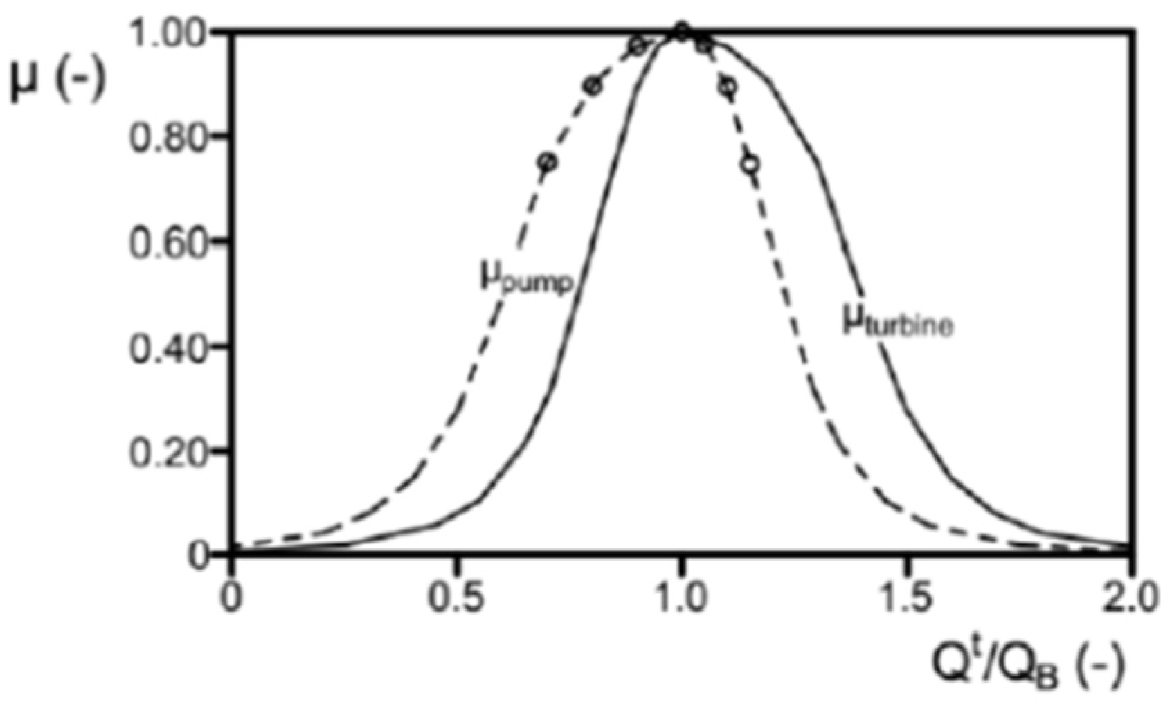
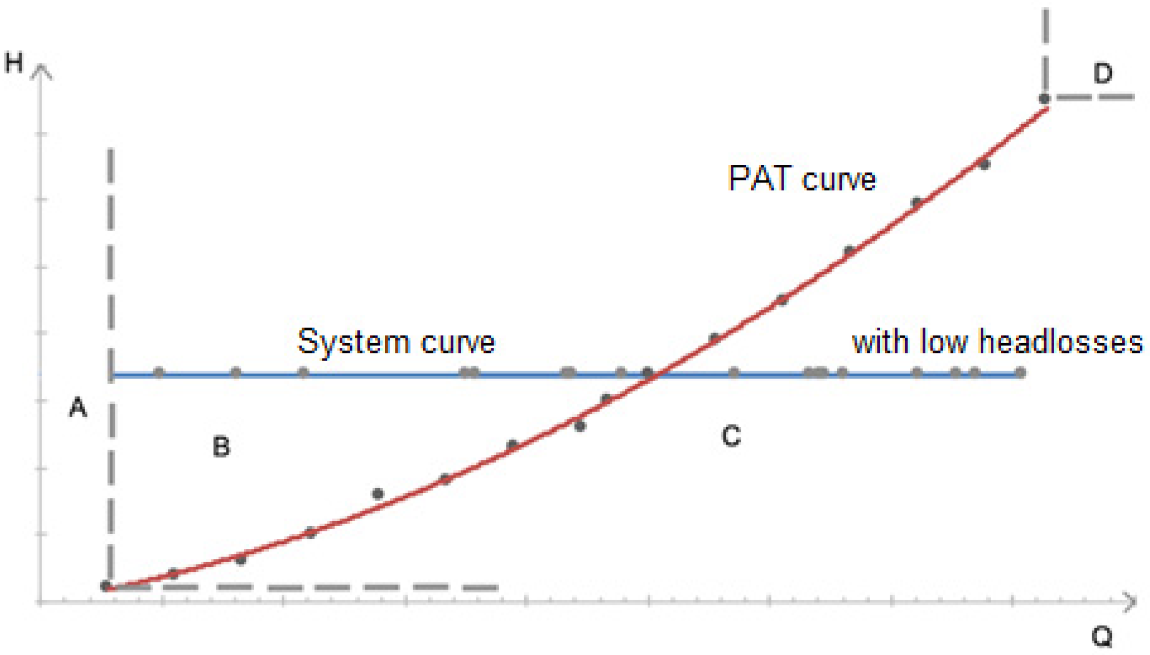
2.1. Fundamentals

In the water transmission and distribution pipes of WDN, a relatively large hydraulic power in Water Supply Systems (WSS) can be found. A notable number of economic benefits could be gained if a careful assessment of the energy potential available in the system is carried out [21].

A recent methodology proposed in literature is the Variable Operating Strategy (VOS). Given a flow-head distribution and a network backpressure, this procedure allows for the geometry selection of any energy production devices (EPDs) ensuring highest values of plant efficiency [22].

In order to guarantee a desirable head despite of the variable conditions, the hydropower plant can be modulated by an hydraulic regulation (HR) or electrical regulation (ER). HR consists of two branches in parallel: one branch has a control valve in series with the PAT, while the other branch works as a bypass line and is equipped with a regulation valve, as shown in Figure 1.

According to HR regulation in Figure 1, when the available head ($H^d$) is greater than the head deliberable by PAT ($H^t$), i.e., the operating point is above the characteristic curve, the excess pressure is dissipated by the control valve (A), which is in series with the PAT. Alternatively, if the flow rate within the system ($Q^d$) is greater than the one deliverable by the PAT ($Q^t$), i.e., the operating point is below the characteristic curve, the excess discharge is bypassed. Conversely, with reference to ER operation, the PAT is equipped with an inverter, which adapts the rotational speed according to the variable flow rate and head values. Moreover, there exists a further operation model, that is, HER mode (see Figure 1), which is the combination of HR and ER modes [22,23,24]. This research focuses only on the HR mode.

Nowadays, water industry is affected by strong management issues. Combined efforts from governance, municipalities, and water sector companies have been made as a consequence of detriments caused by climate change, population growth, and urbanization, in order to find adaptive solutions in moving towards sustainability.

To increase the efficiency and lower the cost in WDN, the current interest leans towards the Smart Water Technologies (SWT), such as Smart Water Grids. Advanced technologies in SWGs, such as smart water pipes and sensors, GIS and/or SCADA platforms, are very effective to assess the quality of water supply service, as well as to monitor and identify any cruciality in WDNs [7,25,26]. The major drawbacks of SWG implementation come with its investment and financing, as well as with political and institutional issues [2,7]. Since the relationship between water and energy is emphasized by the water-energy nexus [27], an integrated sustainably efficient management network can be achieved by the combination of the water-energy nexus and a deep knowledge in SWG.

2.2. Methods

Equation (1) shows the network effectiveness (E), which is a crucial measure to assess the viability of a given strategy. According to Equation (1), the effectiveness of a strategy depends on its capability (${\eta }_p^i$), reliability (${\mu }_p^i$) and sustainability (${\chi }_p$). The ratio of the produced electric energy to the available hydraulic energy, for a given demand pattern, is the system capability and it is given by Equation (2).

$$E={\eta }_p^i{\chi }_p{\mu }_p^i$$

(1)

$${\eta }_p^i=\frac{{{\displaystyle \sum }}_{i=1}^n{H}_i^t{Q}_i^t{\eta }_i^t∆t_i}{{{\displaystyle \sum }}_{i=1}^n{H}_i{Q}_i∆t_i};Q_i^t\le Q_i,H_i^t\le H_i$$

(2)

With reference to Equation (2), $n$ is the number of points in the operating zone, $Q_i^t$ is the PAT discharge $({\mathrm{m}}^3/\mathrm{s})$, $Q_i$ is the discharge within the pipe $({\mathrm{m}}^3/\mathrm{s})$, $H_i^t$ is the head drop through the PAT (m), $H_i$ is the head needed for regulation $\left(\mathrm{m}\right)$, $∆t_i$ is the time interval with constant hydraulic values $\left(\mathrm{h}\right)$ and ${\eta }_i^t$ is the PAT efficiency.

The probability of the functioning of a network component without failure for a given period of time is expressed represents the reliability. Equation (3) provides a general expression of reliability ($R$) using an exponential probability distribution.

$$R\left(t\right)=e^{-\lambda t}$$

(3)

In Equation (3), λ is the failure rate and it is given by the inverse of the Mean Failure Time (i.e., 1/MFT).

With reference to the PAT system, the reliability can be expressed according to Equation (4), as a function of the flow rate of the PAT at the best efficiency point (BEP).

$${\mu }_p^i=\frac{MFT\left(\raisebox{1ex}{$Q$}\!\left/ \!\raisebox{-1ex}{$Q_{BEP}$}\right.\right)}{MFT\left(Q_{BEP}\right)}$$

(4)

According to Equation (4), the more the PAT operating point being closer to its BEP, the higher the reliability value [4,24].

A standard curve for the reliability is given in Figure 2.

Equation (5) [23] provides the expression for sustainability $\left({\chi }_p^i\right)$, which accounts for the reduction in effectiveness when the deliverable head and available head are different from each other.

$${\chi }_p^i={\left(1+10\frac{\left|H^t-∆H^d\right|}{BP}\right)}^{-1}$$

(5)

In Equation (5), $BP$ is the backpressure $\left(\mathrm{m}\right)$, $∆H^d$ the available head in the system $\left(\mathrm{m}\right)$ and $H^t$ the head delivered by the PAT $\left(\mathrm{m}\right)$ [23].

In this study, a methodology for increasing the effectiveness of water distribution networks is proposed. Figure 3 shows a flow-chart of the proposed methodology.

The methodology adopted, which encompasses the implementation, calibration and optimization processes, is crucial in obtaining reliable results. The proposed methodology relies on three main stages: (i) Data collection and calibration of the digital model; (ii) Use of the calibrated model to assess the benefits resulting from the installation of PRVs and PATs, in terms of energy efficiency and leakage reduction; (iii) assessment of the feasibility of the proposed solution based on technical and economic analyses.

Data referring to the spatial layout (length and elevation) and physical characteristics (type of material, diameter, state of conservation, among others) of conduits, connection nodes, final consumption nodes, as well as all hydraulic equipment, which include the reservoir and valves essential for the materialization of the network in computer support, are acquired in GIS format from the Water Management Entity. The data was imported directly into the WG using the ModelBuilder tool, where the parameters required for its complete definition are matched to each type of network infrastructure. For the tuning and calibration study, the consumption pattern represents the flows recorded in 1 h plots during 365 days; for the evaluation of the energy use solution, three patterns of average daily consumption are created. The results of the Digital Twin model are thus evaluated, using the comparison of pressure values at monitoring points with the values obtained by the Management Entity, based on the stated assumptions for estimating consumption. The aim is to make benchmark analysis for periods of different consumption. Data analysis and calibration allow drawing the first conclusions of the study in terms of pressure and flow distribution. In order to be able to quantify the residual recoverable energy of the system, carrying out its energy balance, it is still necessary to optimize it, in order to find solutions that can be studied. The optimization consisted of the following steps:

• Opening of closed PRVs;
• Setting the minimum pressure downstream of the existing PRVs, with the criterion of verifying the minimum regulatory pressure at the critical points of the network.
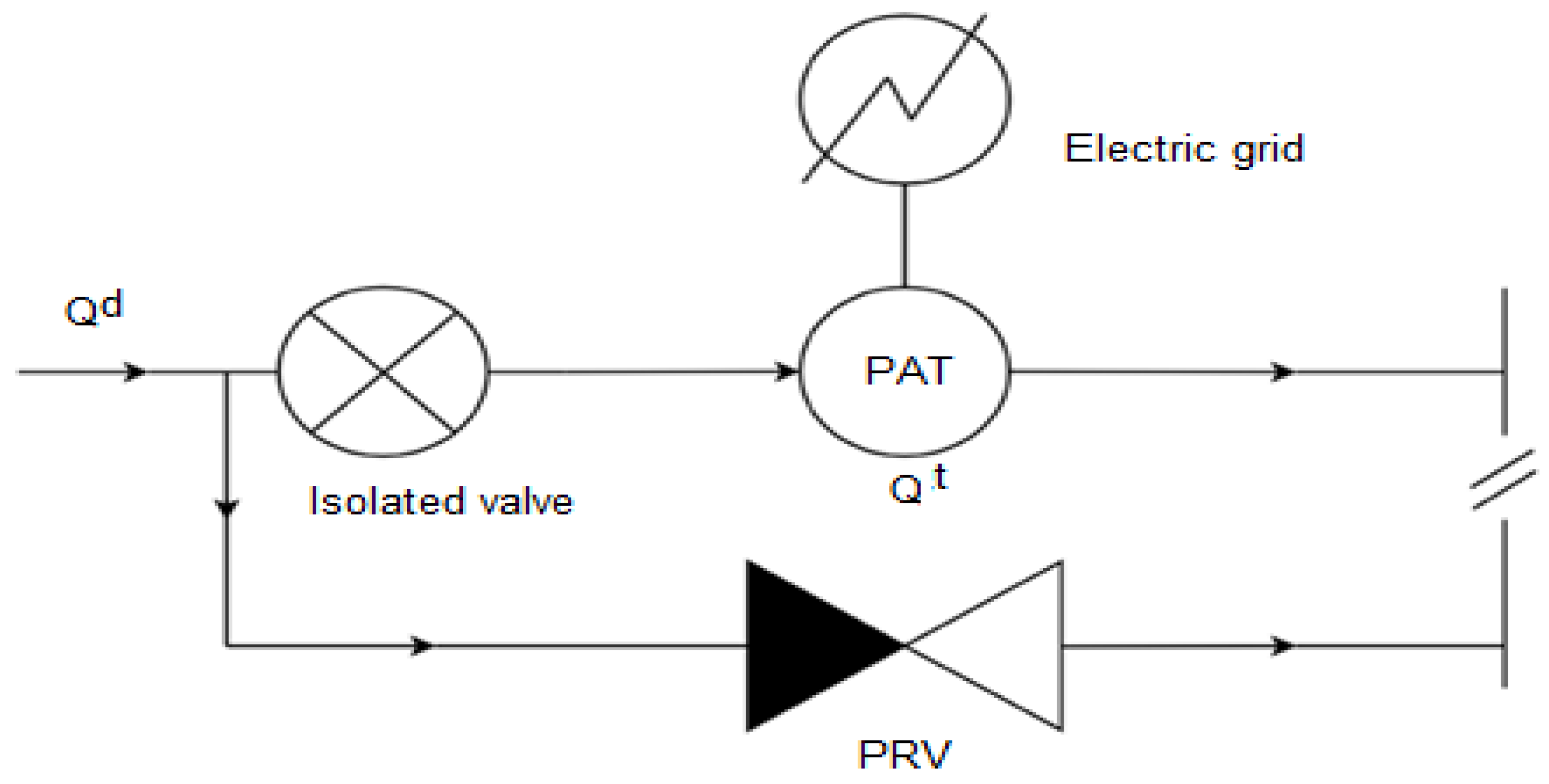
• Implementation of two new PRVs, in a strategic location, in order to control pressure on the network and simultaneously study their possible energy use.
• Evaluation of the network leakage simulation.

The strategic vision of the Management Entity includes an effort to measure and control flow data, a system having recently been incorporated, Waternet, which returns various network performance indicators, which are mainly used in the immediate detection of leaks and real losses, improving the efficiency of systems and the costs associated with water loss. Once an adequate level of guarantee has been achieved in the modelling, and in accordance with the existing hydraulic constraints, namely the regulations and ranges of flow values and operating head of the pumps in turbine mode, the construction of scenarios and alternatives to be taken into account in the energy assessment, for each period of existing consumption. For each scenario, the best PAT curve is evaluated in order to better adapts to the hydraulic conditions of the network, i.e., installed flow and pressure. An analysis of the efficiency of the system is carried out, as well as the Effectiveness (E), capability (${\eta }_p^i$), reliability (${\mu }_p^i$) and sustainability (${\chi }_p^i$), as well as an energy and economic analysis, which leads to the most reliable solution.

2.2.1. Model Restrictions

WDNs are required to fulfill both velocity and pressure criteria.

The maximum flow velocity ($V_{max}$) within a pipe is defined in Equation (6).

$$V_{max}=0.127D^{0.4}$$

(6)

where $D$ is the internal diameter of the pipe $\left(\mathrm{mm}\right)$. Moreover, the velocity is required not to assume value less than 0.3 m/s. In case such minimum requirement is not met, discharge valves are required.

Besides velocity, pressure conditions should be also verified. The maximum service pressure must not exceed 600 $\mathrm{kPa}$ while the maximum pressure fluctuation must not exceed 300 $\mathrm{kPa}$. Moreover, the minimum service pressure is defined in Equation (7):

$$p_{min}=100+40n$$

(7)

where $p_{min}$ is the minimum pressure $\left(\mathrm{kPa}\right)$ and $n$ is the number of floors above ground level, including the ground level $\left(-\right)$ [28,29,30].

In hydraulic regulation mode, when the head upstream of the PAT is higher than the deliverable value, a regulating valve dissipates the excess pressure. Conversely, if the flow rate is too high, the regulating valve dissipates the excess flow. In this mode of operation, the PAT rotation speed is assumed as fixed. The hydraulic regulation modelling is presented in Equation (8):

$$\left\{\begin{array}{c}{H}^d=H^t\left(Q^t\right)+H_{valve}\\ Q^d=Q^t+Q_{bypass}\\ \begin{array}{c}{H}_{valve}>0,Q_{bypass}=0 if H^t\left(Q^t\right)<H_d\\ H_{valve}=0,Q_{bypass}>0 if H^t\left(Q^t\right)>H_d\end{array}\end{array}\right.$$

(8)

where $H^d$ is the available head drop (m), $H^t$ is the head drop within the PAT (m), $H_{valve}$ is the head drop within the regulation valve (m), $Q^d$ is the flow rate within the system (L/s), $Q^t$ is the turbined flow (L/s) and $Q_{bypass}$ is the flow through the regulation valve (L/s).

The energy produced in the hydraulic regulation mode is dependent on the characteristics of the system and the selected PATs. Figure 4 presents the four operating regions of a system based on PAT technology.

According to Figure 4, there exist four operating zones:

$$\begin{gathered} \mathrm{Zone}\mathrm{A}—Q^d<Q_{min}^{t}or{H}^d<H_{min}^t:E_p=0 \\ \mathrm{Zone}\mathrm{B}—Q_{min}^t<Q^d<Q_{max}^{t}and{H}^d>H^t\left(Q^d\right):E_p=P\left(Q^d\right)∆t_i \\ \mathrm{Zone}\mathrm{C}—Q_{min}^t<Q^d<Q_{max}^{t}and{H}_{min}^t<H^d<H_{max}^t:E_p=P\left(Q^d\left(H^d\right)\right)∆t_i \\ \mathrm{Zone}\mathrm{D}—Q^d>Q_{max}^{t}and{H}^d>H_{max}^t:E_p=P\left(Q_{max}^t\right)∆t_i \end{gathered}$$

(9)

According to Equation (9), $Q_{min}^t$ is the minimum flow turbined by the PAT (L/s), $Q_{max}^t$ is the maximum turbined flow within the PAT (L/s), whereas $H_{min}^t$ and $H_{max}^t$ are, respectively, the minimum and maximum head drops within the PAT (m). Moreover,$P$ is the power (W) and $∆t_i$ is the operating time interval (h).

The characteristics of the selected PAT, assuming the engine rotation speed fixed at 1520 rpm, are presented in

Table 1. Selected PAT characteristics.

PAT	${\mathit{Q}}_{\mathit{m}\mathit{i}\mathit{n}}^{\mathit{t}}\left(\mathit{l}/\mathit{s}\right)$	${\mathit{Q}}_{\mathit{m}\mathit{a}\mathit{x}}^{\mathit{t}} \left(\mathit{l}/\mathit{s}\right)$	${\mathit{H}}_{\mathit{m}\mathit{i}\mathit{n}}^{\mathit{t}} \left(\mathit{m}\right)$	${\mathit{H}}_{\mathit{m}\mathit{a}\mathit{x}}^{\mathit{t}}\left(\mathit{m}\right)$	${\mathit{Q}}_{\mathit{B}\mathit{E}\mathit{P}}\left(\mathit{l}/\mathit{s}\right)$	${\mathit{H}}_{\mathit{B}\mathit{E}\mathit{P}} \left(\mathit{m}\right)$	${\mathit{\eta }}_{\mathit{i}}^{\mathit{t}} \left(-\right)$
Etanorm 32–160	3.33	7.31	11	34	5.55	21	0.6
Etanorm 40–200	5.56	13.4	16	52.5	10	32	0.57

.

With reference to Table 1, $Q_{BEP}$ and $H_{BEP}$ represent, respectively, the flow rate and the head drop of the PAT at the best efficiency point.

2.2.2. Hydraulic-Energy Simulator Model

Hydraulic simulation enables a deep analysis of pressure for leakage control and energy recovery. In this study, WaterGEMS (WG) software has been used to carry out the hydraulic simulations and investigate the behavior of the system. This software was developed by Haestad Methods and distributed by Bentley Systems [31].

WaterGEMS relies on the principles of Conservation of Mass and Conservation of Energy to solve the hydraulic equilibrium of a water system. Based on the Gradient Algorithm, this solver allows to solve the network, whether in steady-state conditions or in Extended Period Simulation (EPS).

Conservation of Mass is applied by the software in network nodes, according to Equation (10):

$$\sum Q_{IN}∆t=\sum Q_{OUT}∆t+∆V_S$$

(10)

where $Q_{IN}$ is the total inflow at the node $\left({\mathrm{m}}^3/\mathrm{s}\right)$, $Q_{OUT}$ is the total demand at the node $\left({\mathrm{m}}^3/\mathrm{s}\right)$, $∆t$ is the time interval $\left(h\right)$ e $∆V_S$ is the change in storage volume $\left({\mathrm{m}}^3\right)$.

Given two nodes of the system, the energy equation can be formulated as:

$$\frac{p1}{\gamma }+z_1+\frac{U_1^2}{2g}=\frac{p2}{\gamma }+z_2+\frac{U_2^2}{2g}+h_l$$

(11)

where $p$ is the pressure $\left(\mathrm{N}/{\mathrm{mm}}^2\right)$, $\gamma$ is the water specific weight $\left(\mathrm{N}/{\mathrm{m}}^3\right)$, $z$ is the pipe elevation $\left(\mathrm{m}\right)$, $U_i$ is the velocity $\left(\mathrm{m}/\mathrm{s}\right)$, $g$ is the gravitational acceleration $\left(\mathrm{m}/{\mathrm{s}}^2\right)$ and $h_l$ the total losses $\left(\mathrm{m}\right)$.

2.2.3. Potential Energy Model

PAT and PRV implementation are both taken into account within the strategy proposed in this study.

PAT efficiency (${\eta }_i^t$) is defined by the ratio between mechanical power ($P_m$) and hydraulic power $(P_h$), as shown in Equation (12) [32]:

$${\eta }_i^t=\frac{P_m}{P_h}=\frac{\mathsf{\omega }\mathsf{\Gamma }}{\mathsf{\gamma }{Q}^t{H}_u}$$

(12)

where $\gamma$ is the water specific fluid $\left(\mathrm{N}/{\mathrm{m}}^3\right)$, $Q^t$ is the PAT discharge $\left({\mathrm{m}}^3/\mathrm{s}\right)$, $H_u$ is the available head $\left(\mathrm{m}\right)$, $\omega$ is the angular velocity $\left(\mathrm{rad}/\mathrm{s}\right)$ and $\Gamma$ is the torque $\left(Nm\right)$.

In this study, PAT characteristic curves were obtained using catalogues provided by KSB manufacturer (Figure 5a). As a complement to PATs, the pressure control strategy will be performed in this study by means of PRVs as well. (Figure 5b).

Given a demand pattern, the energy production can be expressed as:

$$E_p=\sum \eta \gamma Q^t{H}_u∆t=\sum P_u∆t$$

(13)

where $E_p$ is the produced energy $\left(\mathrm{kWh}\right)$, $P_u$ is the produced power $\left(\mathrm{kW}\right)$ and ${∆}_t$ is the time interval $\left(h\right)$.

2.2.4. Economic Model

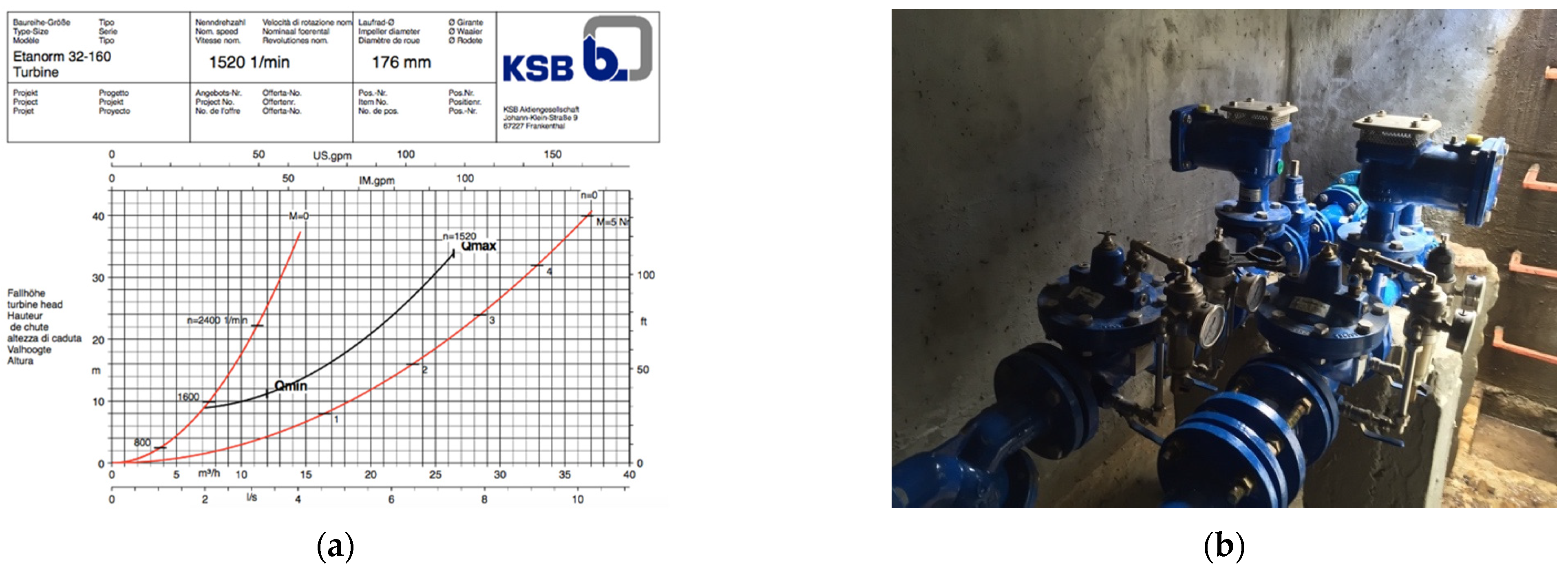
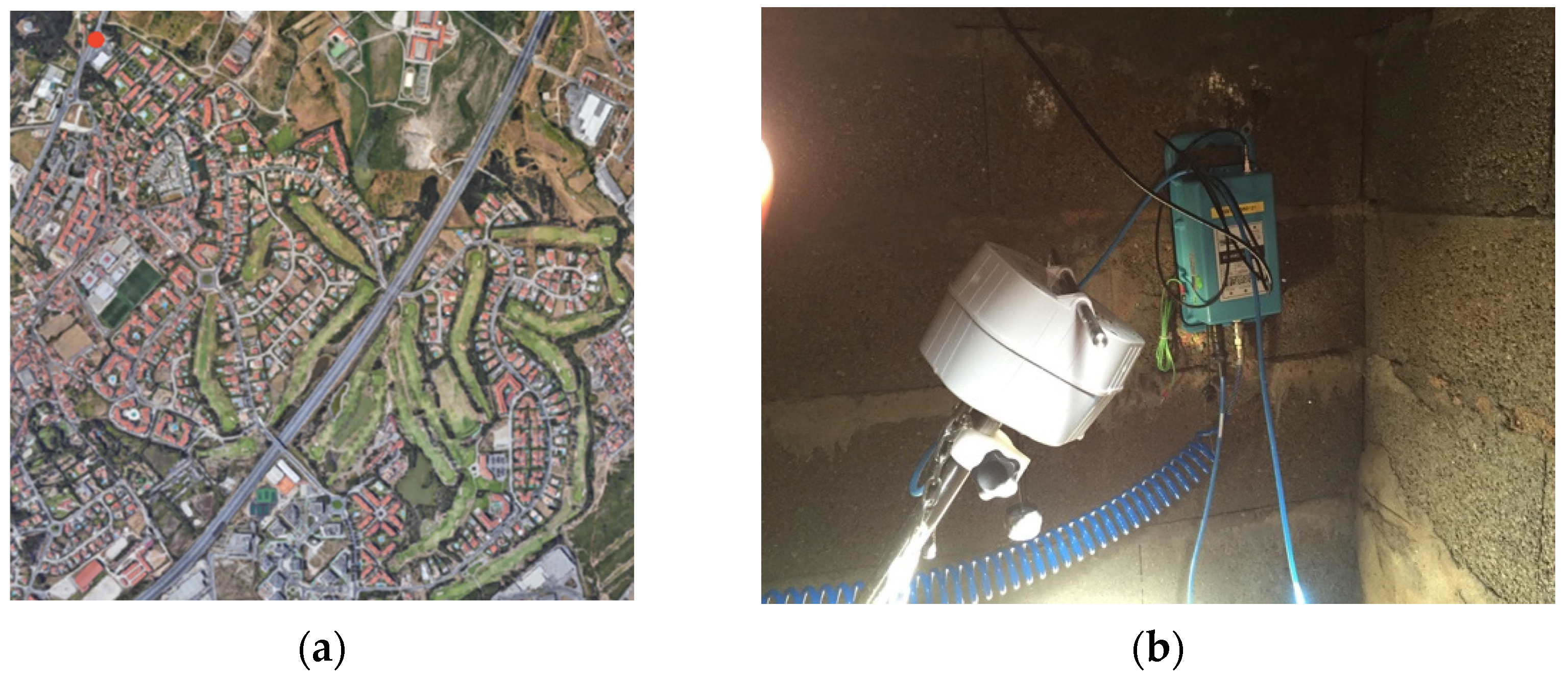
An economic analysis has been carried out in order to assess the viability of the proposed strategy. The criteria for selecting a strategy cannot be merely the maximization of the energy revenue. As a matter of fact, the solution that leads to greater economic benefit may not be the solution that optimizes cost-effectiveness. Thus, the most viable solution should be carefully investigated, based on a comparative analysis between different economic criteria.

The assessment is carried out using and comparing several economic functions, such as the Net Present Value $\left(NPV\right)$, benefit-cost ratio ($B/C)$, internal rate of return $\left(IRR\right)$ and payback period $\left(PBT\right)$.

$NPV$ formulation is presented in Equation (14), where it is expressed as the cumulative sum of revenue minus costs during the lifetime of the project.

$$NPV=R-C-O-P$$

(14)

With reference to Equation (14),  $R$ is the revenue, $C$ is the capital cost, $O$ is the operation cost and $P$ is the reposition cost. The greater the $NPV$, the more attractive the solution.

The $B/C$ function represents the ratio between present value of benefits and total costs, as shown in Equation (15):

$$B/C=\frac{R-O}{C+P}$$

(15)

The greater the ratio, the more attractive the solution. For $B/C$ ratio values smaller than 1, projects are considered unviable.

The internal rate of return, $IRR$, represents instead the discount rate that makes $NPV$ equal to zero. The greater the $IRR$, the better the solution. Finally, the payback period, $PB$, represents the number of years until the cumulative cash-flows turn positive, that is, the number of years until revenue surpasses the costs [33].

3. Case Study

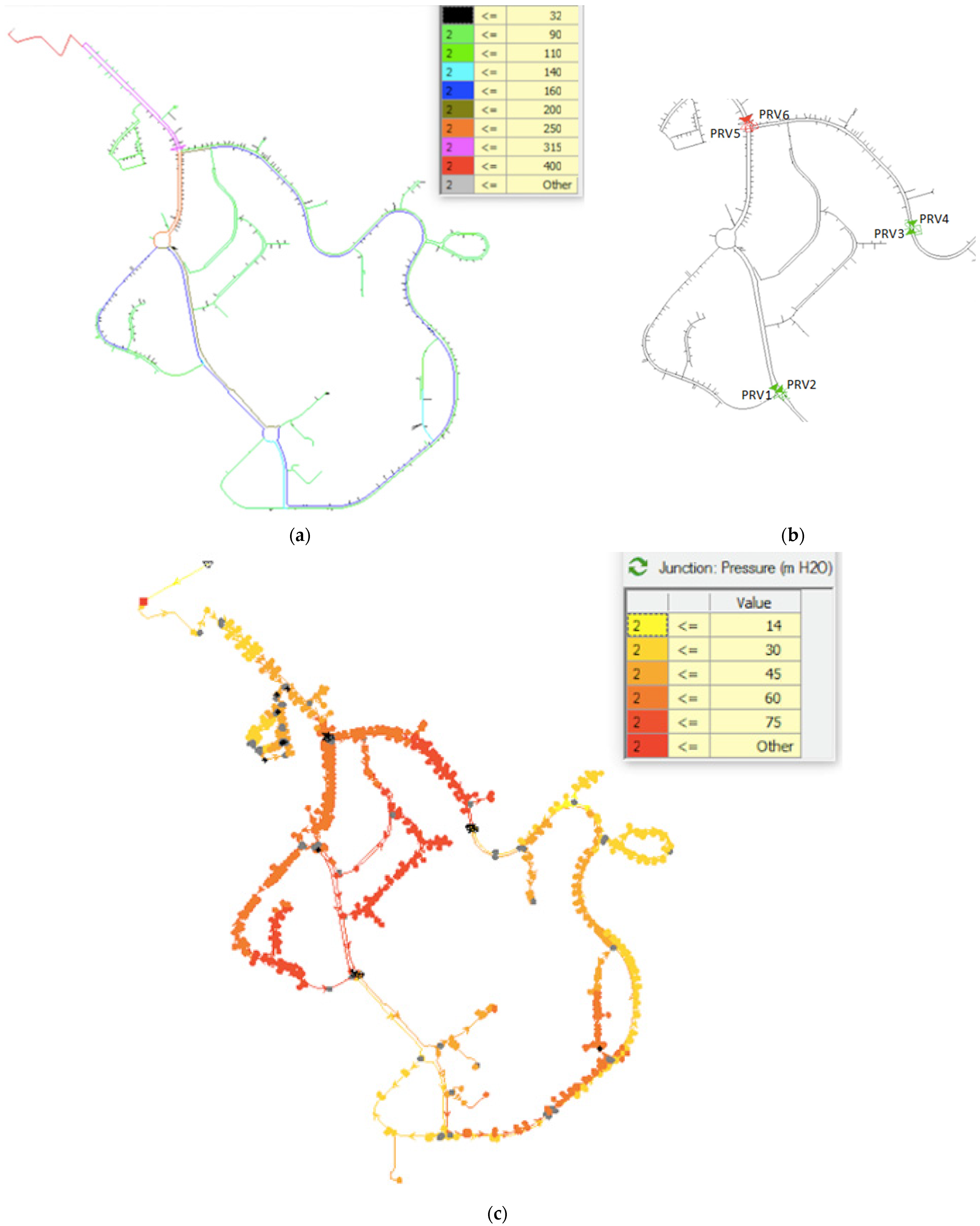
3.1. Brief Description

The Sintra Municipal Water and Sanitation Services (SMAS) is one of the largest water distribution authority in the country, with around 182,000 customers spread over 320 km². The SMAS is responsible for managing water in the municipality of Sintra, with a distribution network that extends over 1784 km of water pipes, divided into 52 DMAs, including Quinta da Beloura, in the Parish of Sintra. Beloura’s DMA, built in the early 2000s, includes 15.4 km of water pipes and serves a population estimated at around 4000 inhabitants, corresponding to 1335 customers. The Management Entity proposed to verify the diameter of pipes, in order to assess their correct dimensioning, as well as a study of the level of pressures and flow velocities in the network and possible improvements to be implemented. On the other hand, it was proposed to evaluate the capacity of the network to produce electricity, through the use of the available hydraulic potential. This study does not take into account water quality assessment, as well as the system behavior in fire situation.

Beloura DMA is equipped with Hydrins flow meter (with an error of +/−1%), which is installed upstream of the water distribution network (Figure 6a) and is used by the Management Authority to register the flow every one-hour intervals. Data are recorded and sent via GSM to a computer system by means of a Multilog data-logger (Figure 6b). This study relies on the values recorded by this measure system and, in particular, focuses on an average one-year period.

With regard to the reference period, the average annual recorded flow is 12.12 L/s, which corresponds to an average capitation of around 260 l/day. It is worth noting that this high value stems from the specific use of the analyzed DMA, which is not merely residential, due to the presence of many services. The annual hourly consumption pattern, which expresses the ratio between the recorded hourly flow rate, $Qi$, and the average annual flow rate, $Qma$, is presented in Figure 7.

According to the recorded data, the hourly consumption ranges between 1.5 and 43 L/s, due to the high seasonal variability of water consumption. Figure 8a shows the frequency of occurrence of the recorded data for the reference period, as well as the cumulative percentage of the total water volume for each level of consumption. By analyzing the data at monthly intervals., three large groups of consumption have been identified: (1) normal, (2) high and (3) very high. The consumption defined as normal aggregates the water utilization registered in the months from November until April (Figure 8b); high consumption refers to months of May and October (Figure 8c); finally, very high consumption refers to the consumption recorded in the months from June until September (Figure 8d).

Once these three scenarios of annual consumption have been defined, a weekly analysis is carried out, in order to obtain different consumption patterns. Figure 9 shows the average hourly data during one-week period, with reference to normal (a), high (b) and very high (c) consumptions.

The network is supplied entirely by gravity from Linhó reservoir, which in turn is supplied from the Ranholas pumping station. The reservoir has a capacity of 4000 m³ and its water level is assumed constant in this study. More specifically, the distribution network consists of two main large pipeline sections—external and internal circular—where 587 branches are connected.

The nominal diameters of the pipes are represented in the network diagram, with values expressed in millimeters. The diameters of the final connection branches vary between 32 and 90 mm (Figure 10a)

According to Figure 10c, most of the network exhibits pressures higher than the maximum allowed, which is between 65 and 70 m w.c. (see red zone in Figure 10c), and much higher than the minimum pressure fixed at 15 m w.c. Indeed, according to the real configuration shown in Figure 10b, the network consists of six PRVs, of which only two work properly, in constant load mode. With reference to PRV1, the valve type is Flucon200.02.03 (DN 100), installed in a 200 mm pipe diameter and set with a downstream pressure value equal to 34 m w.c. Instead, PRV2 is a Flucon200.02.03 (DN65) and it is installed in a 140 mm pipe diameter, with a pressure set equal to 15 m w.c. According to the current configuration, all the other PRVs (Flucon200.02.03 DN65) are closed. In this study, the pressure values are adjusted, assuming constant load regulation mode. In particular, PRV1 and PRV2 are set with a downstream pressure value of 15 m w.c., PRV3 and PRV4 are set with a downstream pressure value of 17 m w.c., while PRV5 and PRV6 are assumed to work with downstream pressure equal to 15 m w.c. According to this setting, the minimum pressure of 14 m w.c. is respected in all network nodes.

3.2. Results

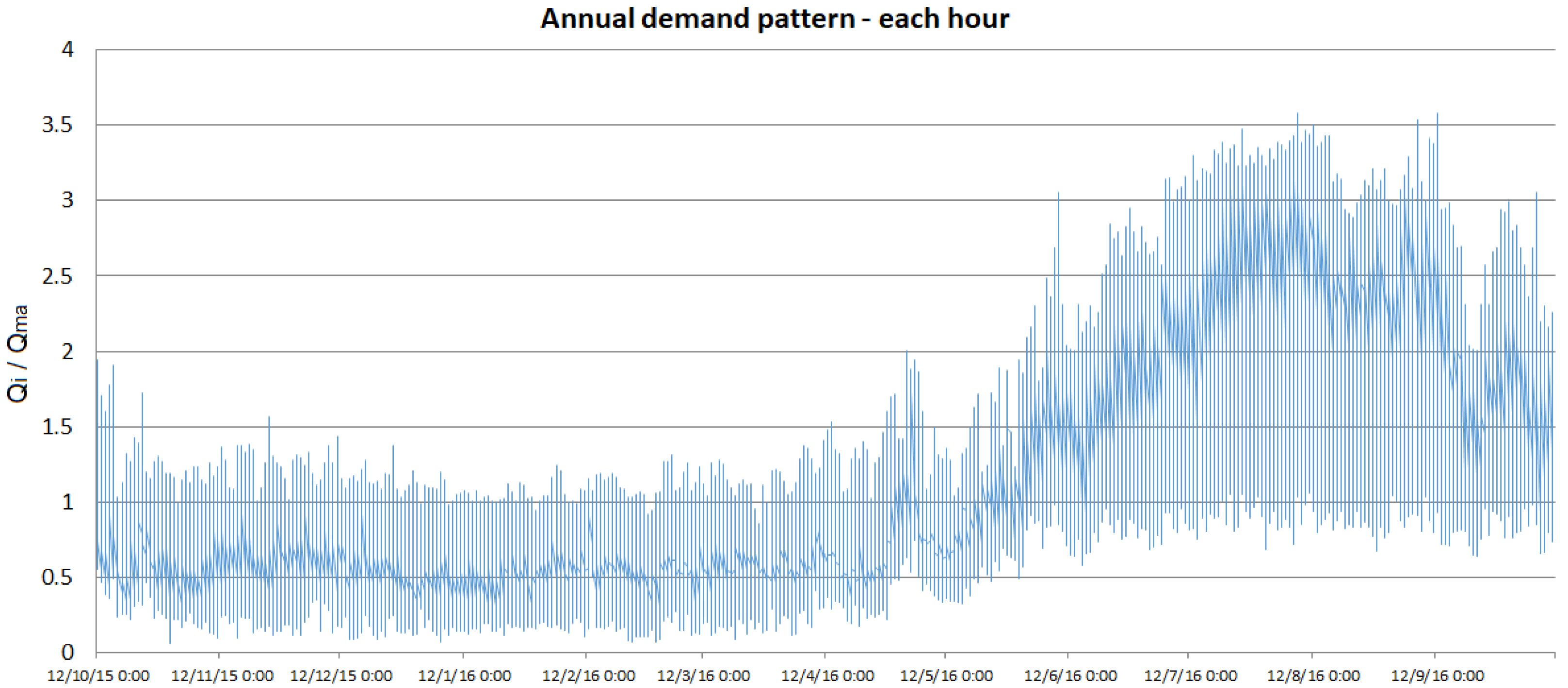
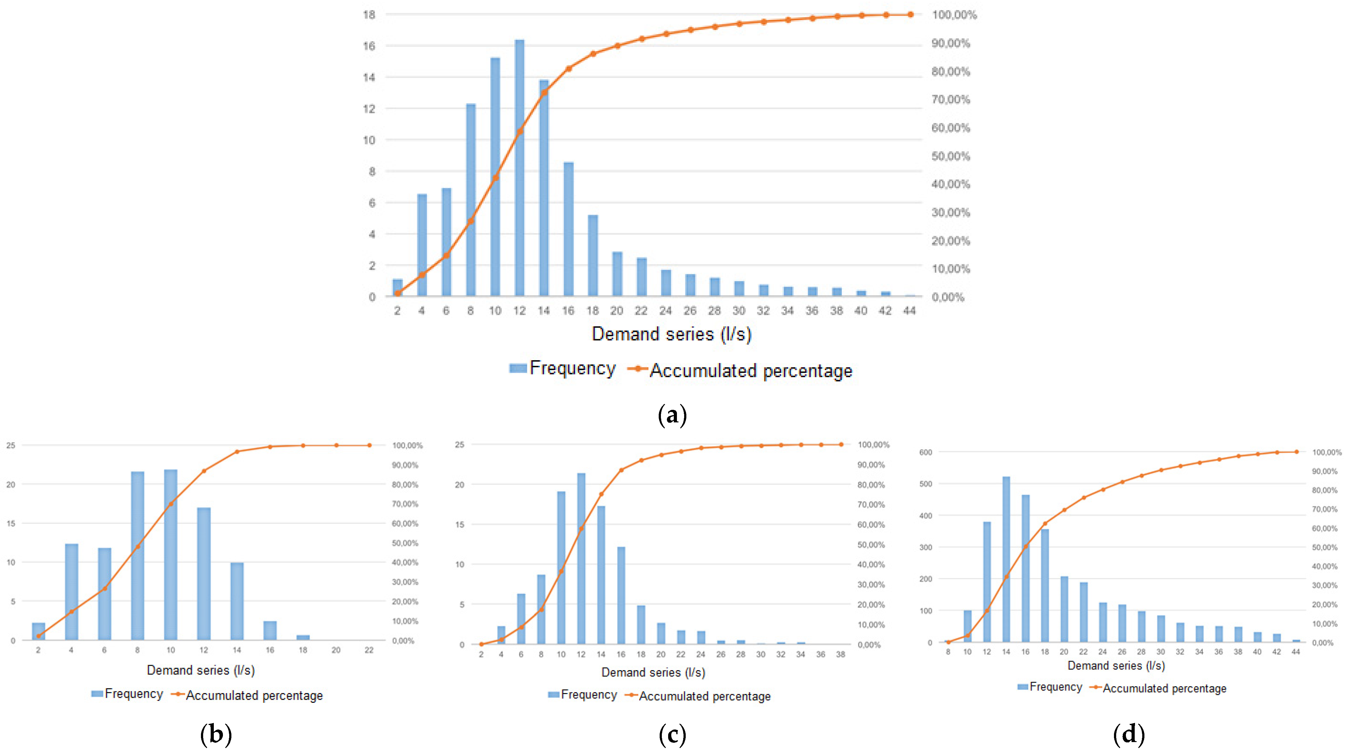
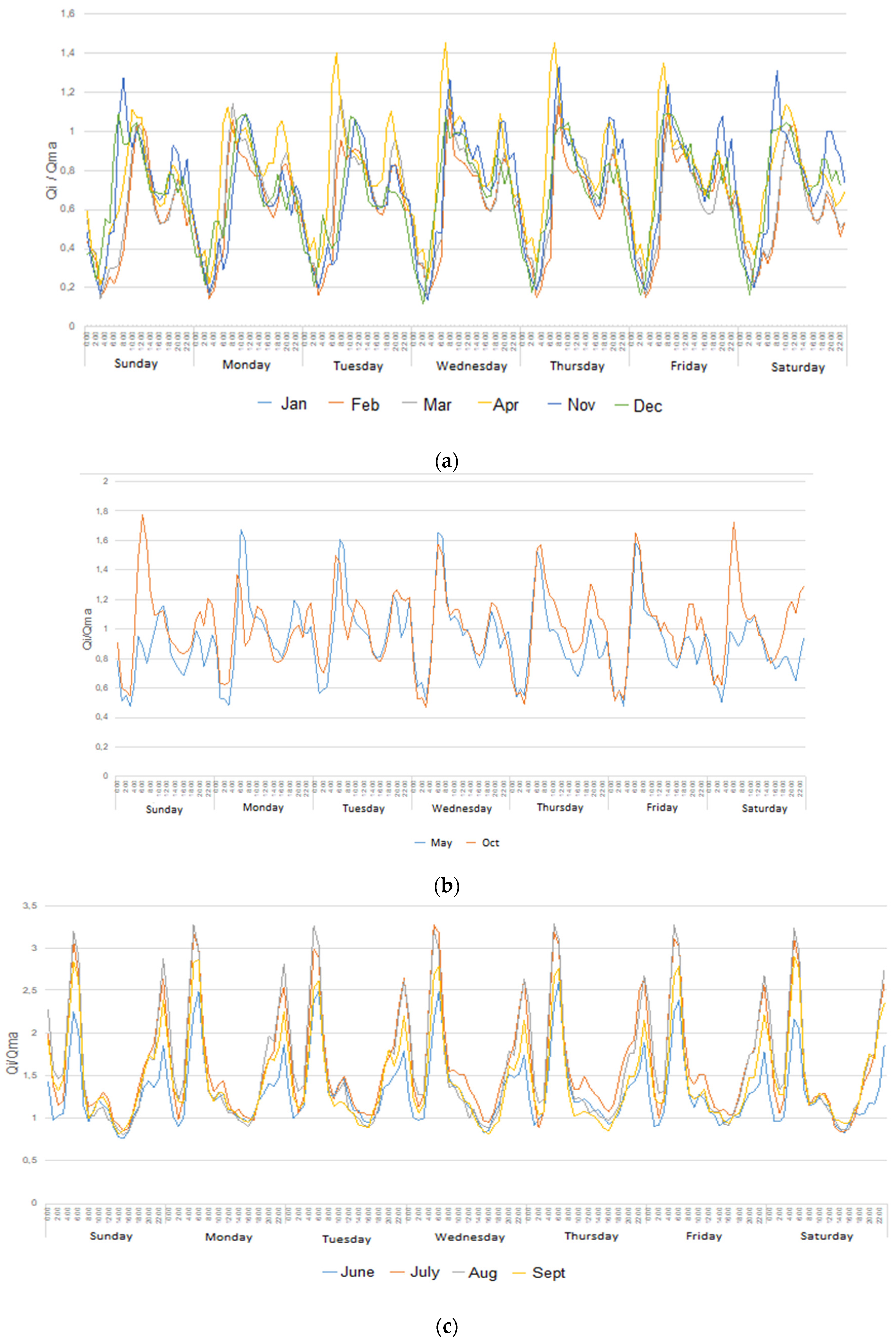
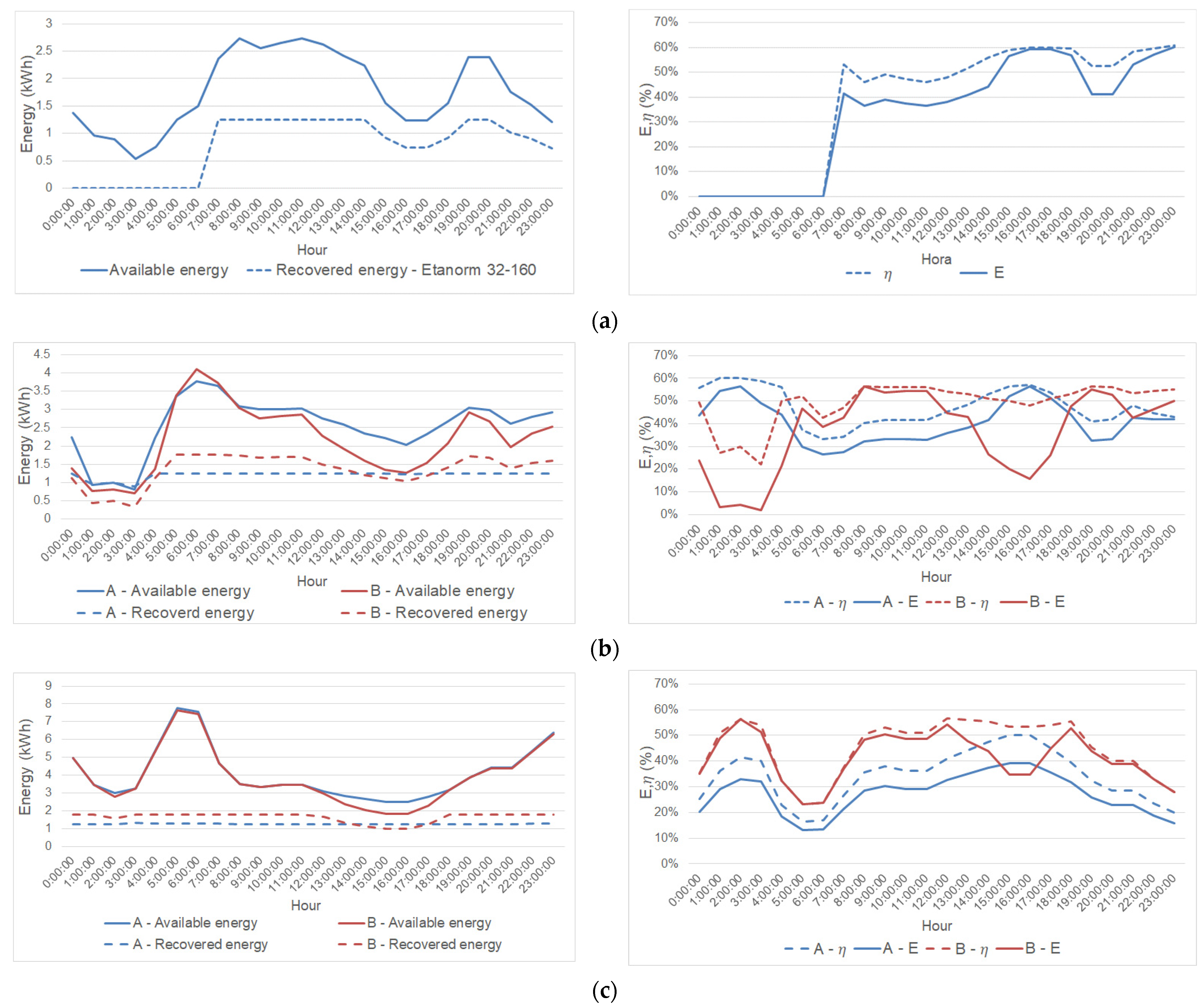
3.2.1. Different Types of Demand Pattern

The results of the hydraulic simulations are presented in Figure 11, with reference to normal (a), high (b) and very high (c) consumption. According to the performed analyses, the value of the flow within PRV3 is null. Moreover, since the flows within the other PRV1, PRV2, PRV4 and PRV5 are very low, these locations are not suitable for PAT installation. Conversely, due to the larger value of flow rate within PRV6, it may be replaced with a PAT.

3.2.2. Water Losses Evaluation

The water network has been recently equipped with Waternet system, which is a useful tool enabling water managers to detect any leaks and losses in the network. According to the measured data, in Beloura’s DMA losses are accounted as around 2.6%, which is low due to the recent age of the system and the good conditions of the pipes.

To perform the hydraulic simulation, the Hazen-Williams roughness coefficient, has been set equal to 140, which is a suitable value for HDPE (High Density Polyethylene) pipelines in good conditions. The simulation has been performed using the “Pressure Dependent Demands” (PDD) function, according which leakage flows are concentrated at the nodes and depend on the pressure values

According to PDD function, there exists an exponential relationship between the leakage flow and the pressure at nodes:

$$Q^l=K\times P_{mo}^n$$

(16)

where $Q^l$ is the leaked flow rate, $K$ and $n$ are, respectively, leakage coefficient and exponent, which depend on the material, the age of the pipes and the shape of the orifice. Finally, $P_{mo}$ is the pressure upstream of the orifice [18]. In this study, $n$ has been assumed as 0.5, which provide realistic values of water leakage within the system.

In this study, for each daily average consumption pattern, the water use has been assumed as distributed equally across the entire network, hence each node is assigned the same probability of occurrence of a leak. This hypothesis offers the most realistic leakage distribution in the network.

For the definition of the individual nodal reference pressure, since the maximum pressure value for which the leakage flow does not depend on the pressure is not known, the daily average values of the pressure in each node was considered corresponding to its network simulation in steady-state mode.

Table 2. Measured flow rates and simulated leakage values for different consumption scenarios.

Types Demand	Average Flow Distributed in the Period  ($\mathrm{L}/\mathrm{s}$)	Daily Leakage Volume (${\mathrm{m}}^3$)	Total Leakage Volume in the Analyzed Period (${\mathrm{m}}^3$)	Yearly Total Leakage Volume (${\mathrm{m}}^3$)
Normal	8.12	30.64	5576	11,623
High	11.74	30.99	1921
Very high	18.28	33.82	4126

presents the average flow values measured by the flow meter system, as well as the leakage values resulting from the performed simulation.

According to Table 2, the simulated leakage amounts on average to around 3.03% of the total flow distributed in the reference year, being therefore in line with expected value. According to this result, the digital model under investigation is properly calibrated and its output values are coherent with the real conditions of the analyzed network. Therefore, the proposed model can be used as a reliable tool to make a realistic assessment of the energy potential and investigate the feasibility of possible energy recovery strategies.

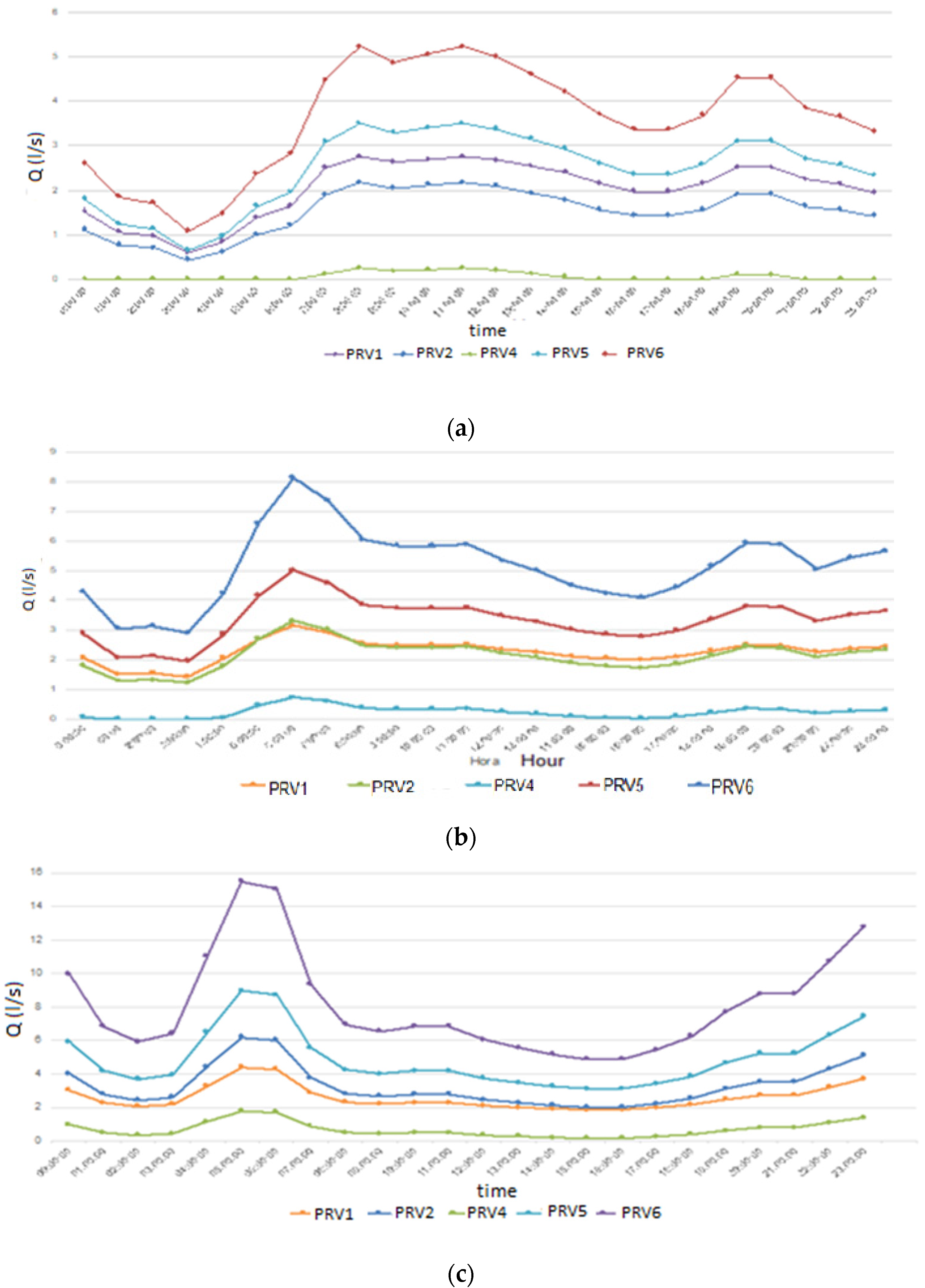
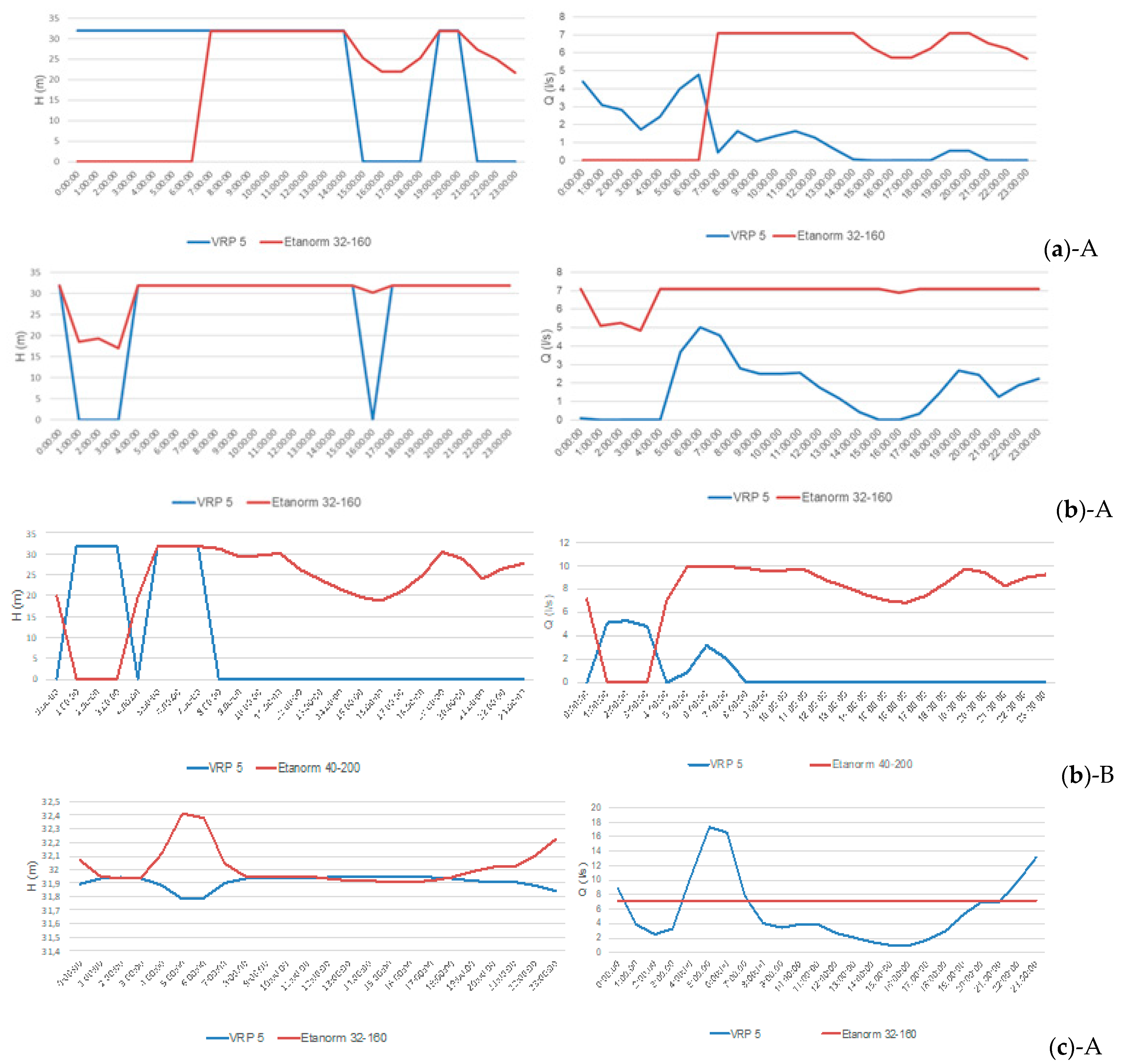
3.2.3. Operating Conditions

In the proposed application, PRV5 is used as a flow control device, instead of a pressure reducing valve. Moreover, a PAT is installed in place of PRV6. Whether the flow is lower or higher than, respectively, the minimum and maximum flow turbined by the PAT, the PRV5 is active and operates in constant load mode. Otherwise, the PRV5 is closed and the flow is entirely turbined by the PAT. The new implementation scheme is then illustrated in Figure 12.

For each different consumption patterns (i.e., normal, high and very high), the behavior of both Etanorm 32–160 and Etanorm 40–200 has been alternatively investigated, as shown in Figure 13.

In Figure 13a (normal consumption), considering Etanorm 32–160 as reference PAT (i.e., alternative A), the maximum useful head drop within the PAT is equal to 31.92 m and the maximum turbine flow assumes value of 7.1 L/s. According to the trend, there is not energy production during night period (i.e., 0–6 am). The maximum pressure resulting from this regulation is equal to 55.3 m w.c. In Figure 13b (high consumption) considering Etanorm 32–160 as reference PAT (i.e., alternative A), the maximum useful turbined head is equal to 31.91 m and the maximum turbined flow is equal to 7.1 L/s. The maximum network pressure is instead equal to 53.1 m w.c. Conversely, assuming Etanorm 40–200 as reference PAT (alternative B) in same consumption scenario, the maximum useful turbined head is equal to 31.91 m and the maximum turbined flow equals to 10 L/s. With regard to the maximum network pressure, this is equal to 55.4 m w.c. In Figure 13c, assuming Etanorm 32–160 as reference PAT (alternative A), the maximum useful turbined head is equal to 32.06 m and the maximum turbine flow is 7.1 L/s, while the maximum network pressure is equal to 46.8 m w.c.. In the same consumption scenario (very high), assuming Etanorm 40–200 as reference machine, the maximum useful turbined head is equal to 31.97 m and the maximum turbine flow takes the value of 10 L/s. The maximum network pressure is, instead, equal to 46.7 m w.c. In all the analyzed scenarios, the reference PATs work closely to BEP values.

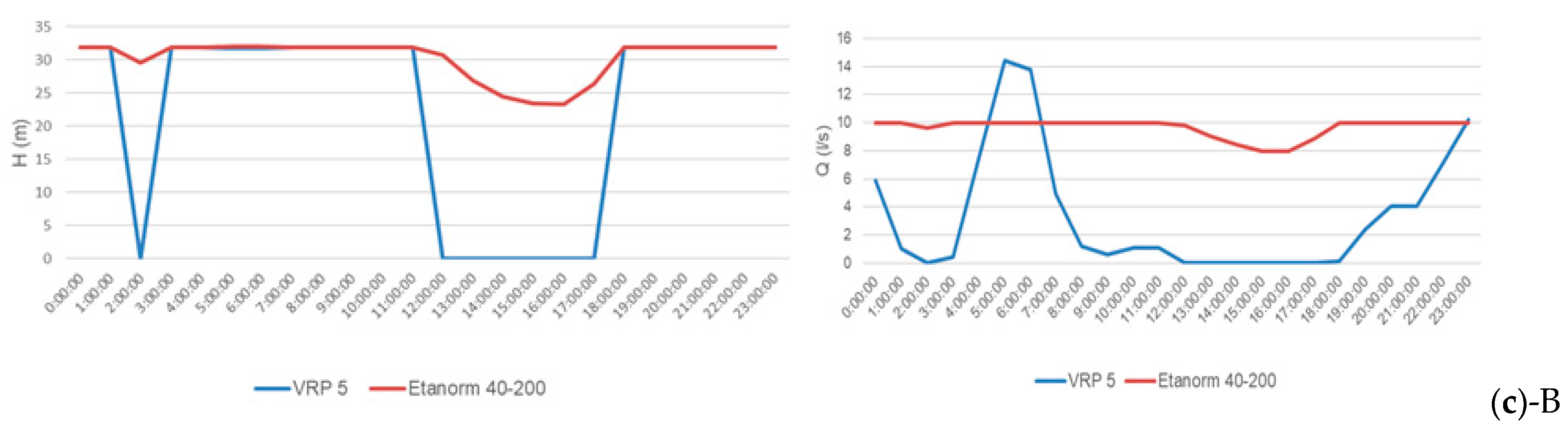
3.2.4. Average Weekly Recovery Energy and System Efficiency

Figure 14 presents the recovered and available energy, as well as effectiveness and capability values, for all the analyzed consumption scenarios. With reference to the normal consumption scenario (see Figure 14a), the maximum value of both effectiveness and capability reaches a values of 59.3%. With regard to the high consumption scenario (Figure 14b), the maximum effectiveness equals to 52.1% and 55.2% for alternatives A and B, respectively. According to the reliability values in alternative B, these are quite low in the intervals 1–3 am and 1–6 pm, as a result of the PAT operating far from its BEP, compared to the remaining time intervals. Moreover, alternative A produces a slightly higher daily energy use (27.8 kWh) compared to alternative B (26.8 kWh). For the very high consumption period, the considered alternatives return maximum capacity values of 52.7% and 56.2% for A and B, respectively. In alternative A, the reduced effectiveness value translates into the poor use of PAT (Etanorm 32–160), which exhausts its production capacity, wasting a lot of energy.

Table 3. Effectiveness ($E$), Capacity (${\eta }_p^i$), Reliability (${\mu }_p^i$) and Sustainability (${\chi }_p^i$) for different consumption scenarios.

Type of Demand	$\overline{\mathit{E}}$   $\left(\%\right)$	${\mathit{E}}_{\mathit{m}\mathit{a}\mathit{x}}$   $\left(\%\right)$	${\mathit{\eta }}_{\mathit{p}}^{\mathit{i}}$   $\left(\%\right)$	$\overline{{\mathit{\mu }}_{\mathit{p}}^{\mathit{i}}}$   $\left(\%\right)$	${\mathit{\mu }}_{\mathit{p}}^{\mathit{i}}{}_{\mathit{m}\mathit{a}\mathit{x}}$   $\left(\%\right)$	$\overline{{\mathit{\chi }}_{\mathit{p}}^{\mathit{i}}}$   $\left(\%\right)$	${\mathit{\chi }}_{\mathit{p}}^{\mathit{i}}{}_{\mathit{m}\mathit{a}\mathit{x}}$   $\left(\%\right)$
Normal	46.9	59.6	53.4	87.4	99.3	98.6	100
High	40.6	56.6	47.5	86.6	99.3	98.2	100
Very high	27.3	39.2	34.3	80	80	99.6	100

presents the average and maximum values of effectiveness ($E$), the capacity (${\eta }_p^i$), reliability (${\mu }_p^i$) and sustainability (${\chi }_p^i$). According to the figures in Table 2, the sustainability reaches the maximum value (100%) in each consumption scenario. With regard to the reliability, it achieves the maximum value in both normal and high consumption scenario, while it decreases to 86.6% for very high consumption scenario.

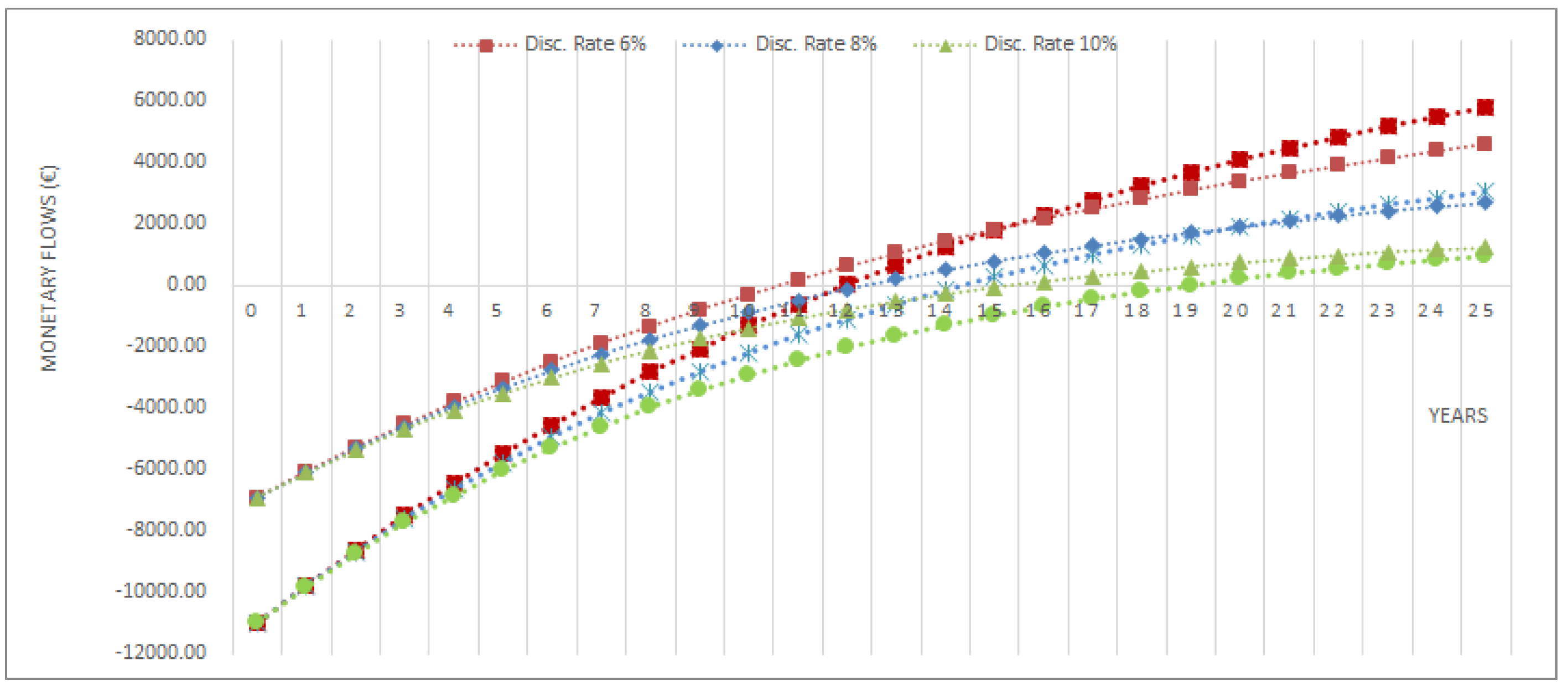
3.2.5. Energetic and Economic Evaluation

According to the obtained results, in the period characterized by normal consumption (i.e., from November to April), the solution consists of a daily production of 18.5 kWh (i.e., 44% of the available energy). In the period of high consumption (May and October), alternative A determines a daily production of 27.8 kWh (45% of available energy) whereas alternative B results in 26.7 kWh (51% of available energy). In the period of very high consumption (from June to September), alternative A ensures a daily production of 30 kWh (30% of available energy) while alternative B guarantees a daily production of 38.8 kWh (41% of available energy). Moreover, if the two PATs (i.e., both Etanorm 32–160 and Etanorm 40–200) are assumed to work in parallel, the energy production results to increase. According to this configuration, Etanorm 32–160 would work for periods of normal and high consumption while Etanorm 40–200 would cover periods of very high consumption, where it has been demonstrated to perform by far better than alternative A. The total efficiency of the system resulting from this configuration would be equal to 37%.

Figure 15 shows the average daily production values resulting from all different consumption scenarios.

In addition, the annual energy production has been also evaluated. In the period of normal demand, the total production reaches 3367 kWh, whereas in the high and very high periods this production amounts to 1725 kWh and 4738 kWh, respectively. Therefore, the total annual production results equal to 9.8 MWh.

The economic analysis has been carried out considering a period of 25 years and assuming an energy selling price equal to 0.1 €/kWh. According to KSB catalogue, the cost of Etanorm 32–160 is equal to 3215 € whereas the Etanorm 40–200 costs 4087 €. With regard to the PRV cost, it has been assessed equal to 2100 €. Moreover, maintenance costs vary significantly, depending on the infrastructure, amounting to 0.5% for civil construction, 2.5% for electrical equipment and 1.5% for hydraulic equipment. Equipment replacement has not been considered within the evaluation, since this cost is expected after 25 years of operation.

Figure 16 shows the monetary flows for different discount rates (i.e., 6%, 8% and 10%), assuming the installation of either one PAT (i.e., Etanorm 32–160) or two PATs (i.e., Etanorm 32–160 and Etanorm 40–200) in parallel. According to this figure, the solution with two PATs result in higher payback period (12 against 9 years) but also in higher NPV value at the end of the simulation period. Moreover, the energy recovery results in lower pressure values, which means leakage reduction. As a result, there is an annual saving of water due to the reduction of leakage amounting to 30%, which correspond to about 3523 m³.

4. Conclusions

Smart water grids (SWG), relying on these digital technologies, allows for a real time monitoring of water networks, with benefits in terms of control of the system, decrease of time response to failures, increase of system sustainability and efficiency.

PRVs are very common solutions used in water networks with the aim of reducing pressure, which is the main cause of water leakage. Moreover, the introduction of a PAT, to replace or supplement PRVs, allows for the transformation of available hydraulic energy into electricity. PATs are becoming increasingly relevant in microscale power production, since its implementation allows to reduce both operational and energy costs, having positive impacts in the systems sustainability.

This research aims at presenting an integrated efficiency management methodology to assess the benefits associated with leakage control and energy recovery, based on the evaluation of system effectiveness ($E$), capability (${\eta }_p^i$), reliability (${\mu }_p^i$) and sustainability (${\chi }_p^i$). Properly calibrated, the developed model allows for a realistic representation of the system conditions in a real water network. The methodology has been tested on Beloura’s DMA (PT), assuming differing consumption scenarios (i.e., normal, high and very high). The behavior of two PATs was investigated, each one representing an alternative for energy recovery in the system. The alternative A, i.e., Etanorm 32–160, was demonstrated to work close to BEP values for normal and high consumption scenarios, whereas the alternative B, i.e., Etanorm 40–200, exhibits its best performance in very high consumption scenario. Moreover, alternative A was demonstrated to ensure a daily production equal to 44%, 45% and 30% of the available energy, for normal, high and very high consumption scenarios, respectively. Conversely, alternative B was proven to save 51% and 41% of the available energy, with reference to high and very high consumption scenarios, respectively. Moreover, assuming the two PATs working in parallel, the annual energy recovered results equal to 9.8 MWh and the reduction of water leakage amounts to 30%, with a payback period of 12 years. On the whole, this solution was demonstrated to be efficient and sustainable, with values of effectiveness ($E$) and capacity (${\eta }_p^i$) up to 50% and 53%, respectively. Moreover, also reliability (${\mu }_p^i$) and sustainability (${\chi }_p^i$) resulted to be promising values, assuming average values up to 87% and 98%, respectively.

This methodology is a useful tool which can find application in a realistic and reliable assessment of the energy efficiency and leakage reduction in any DMAs. It also allows for possible benchmark analysis between different water management entities towards digital transition and sustainable development goals.

References

1. United Nations World Water Assessment Programme (WWAP). The United Nations World Water Development Report 2019: Water for a Sustainable World; UNESCO: Paris, France, 2019. [Google Scholar]
2. Ramos, H.M.; Morani, M.C.; Carravetta, A.; Fecarrotta, O.; Adeyeye, K.; López-Jiménez, P.A.; Pérez-Sánchez, M. New Challenges towards Smart Systems’ Efficiency by Digital Twin in Water Distribution Networks. Water 2022, 14, 1304. [Google Scholar] [CrossRef]
3. Pérez-Sénchez, M.; Sénchez-Romero, F.J.; Ramos, H.M.; López-Jiménez, P.A. Energy Recovery in Existing Water Networks: Towards Greater Sustainability. Water 2017, 9, 97. [Google Scholar] [CrossRef] [Green Version]
4. Carravetta, A.; Giudice, G.D.; Fecarotta, O.; Ramos, H.M. Pump as turbine (PAT) design in water distribution network by system effectiveness. Water 2013, 5, 1211–1225. [Google Scholar] [CrossRef] [Green Version]
5. Thornton, J.; Sturm, R.; Kunkel, G. Water Loss Control; McGraw-Hill Companies: New York, NY, USA, 2008. [Google Scholar]
6. Arregui, F.J.; Cobacho, R.; Soriano, J.; Jimenez-Redal, R. Calculation Proposal for the Economic Level of Apparent Losses (ELAL) in a Water Supply System. Water 2018, 10, 1809. [Google Scholar] [CrossRef] [Green Version]
7. Martyusheva, O. Smart Water Grid; Department of Civil and Enviromental Engineering, Colorado State University: Fort Collins, CO, USA, 2014. [Google Scholar]
8. Đurin, B.; Margeta, J. Analysis of the possible use of solar photovoltaic energy in urban water supply systems. Water 2014, 6, 1546–1561. [Google Scholar] [CrossRef] [Green Version]
9. Walski, T. Committee Report: Defining model calibration. J. Am. Water Works Assoc. 2013, 105, 60–63. [Google Scholar]
10. PENSAAR. Uma Nova Estratégia Para o Setor de Abastecimento de águas e Saneamento de águas Residuais. 2020. Available online: https://apambiente.pt/agua/plano-estrategico-de-abastecimento-de-agua-e-saneamento-de-aguas-residuais (accessed on 10 April 2015).
11. Fabbiano, L.; Vacca, G.; Dinardo, G. Smart water grid: A smart methodology to detect leaks in water distribution networks. Measurement 2020, 151, 107260. [Google Scholar] [CrossRef]
12. Ramos, H.M.; McNabola, A.; López-Jiménez, P.A.; Pérez-Sánchez, M. Smart Water Management towards Future Water Sustainable Networks. Water 2020, 12, 58. [Google Scholar] [CrossRef] [Green Version]
13. Galdiero, E.; De Paola, F.; Fontana, N.; Giugni, M.; Savic, D. Decision support system for the optimal design of district metered areas. J. Hydroinform. 2015, 18, 49–61. [Google Scholar] [CrossRef] [Green Version]
14. Parra, S.; Krause, S.; Krönlein, F.; Günthert, F.W.; Klunke, T. Intelligent pressure management by pumps as turbines in water distribution systems: Results of experimentation. Water Sci. Technol. Water Supply 2018, 18, 778–789. [Google Scholar] [CrossRef] [Green Version]
15. Conejos Fuertes, P.; Martínez Alzamora, F.; Hervás Carot, M.; Alonso Campos, J.C. Building and exploiting a Digital Twin for the management of drinking water distribution networks. Urban Water J. 2020, 17, 704–713. [Google Scholar] [CrossRef]
16. Ulanicki, B.; Bounds, P.; Rance, J.; Reynolds, L. Open and closed loop pressure control for leakage reduction. Urban Water 2000, 2, 105–114. [Google Scholar] [CrossRef]
17. Pastor, A.V.; Palazzo, A.; Havlik, P.; Biemans, H.; Wada, Y.; Obersteiner, M.; Kabat, P.; Ludwig, F. The global nexus of food–trade–water sustaining environmental flows by 2050. Nat. Sustain. 2019, 2, 499–507. [Google Scholar] [CrossRef] [Green Version]
18. Fontana, N.; Giugni, M.; Portolano, D. Losses Reduction and Energy Production in Water-Distribution Networks. J. Water Resour. Plan. Manag. 2012, 138, 237–244. [Google Scholar] [CrossRef]
19. Wu, H.; Jin, R.; Liu, A.; Jiang, S.; Chai, L. Savings and Losses of Scarce Virtual Water in the International Trade of Wheat, Maize, and Rice. Int. J. Environ. Res. Public Health 2022, 19, 4119. [Google Scholar] [CrossRef] [PubMed]
20. Vilanova, M.R.N.; Balestieri, J.A.P. Energy and hydraulic efficiency in conventional water supply systems. Renew. Sustain. Energy Rev. 2014, 30, 701–714. [Google Scholar] [CrossRef]
21. Carravetta, A.; Del Giudice, G.; Fecarotta, O.; Ramos, H.M. Energy production in water distribution networks: A PAT design strategy. Water Resour. Manag. 2012, 26, 3947–3959. [Google Scholar] [CrossRef]
22. Fecarotta, O.; Aricó, C.; Carravetta, A.; Martino, R.; Ramos, H. Hydropower Potential in Water Distribution Networks: Pressure Control by PATs. Water Resour. Manag. 2014, 29, 699–714. [Google Scholar] [CrossRef]
23. Carravetta, A.; Giudice, G.D.; Fecarotta, O.; Ramos, H.M. PAT design strategy for energy recovery in water distribution networks by electrical regulation. Energies 2013, 6, 411–424. [Google Scholar] [CrossRef] [Green Version]
24. Carravetta, A.; Ferracotta, O.; Ramos, H. Energy production by PAT in small residential areas. Renew. Energy, 2016; 1–16, Submitted. [Google Scholar]
25. Boyle, T.; Giurco, D.; Mukheibir, P.; Liu, A.; Moy, C.; White, S.; Stewart, R. Intelligent Metering for Urban Water: A Review. Water 2013, 5, 1052–1081. [Google Scholar] [CrossRef] [Green Version]
26. Byeon, S.; Choi, G.; Maen, S.; Gourbesville, P. Sustainable water distribution strategy with smart water grid. Sustainability 2015, 7, 4240–4259. [Google Scholar] [CrossRef] [Green Version]
27. Kenway, S.J.; Lant, P.A.; Priestley, A.; Daniels, P. The connection between water and energy in cities: A review. Water Sci. Technol. 2011, 63, 1983–1990. [Google Scholar] [CrossRef] [PubMed]
28. Ministério das Obras Pêblicas, Transportes e Comunicações. Decreto Regulamentar nº 23/95, de 23 de Agosto, 36. 1995. Available online: https://dre.pt/dre/detalhe/decreto-regulamentar/23-1995-431873 (accessed on 10 April 2015).
29. Wagner, J.M.; Shamir, U.; Marks, D.H. Water distribution reliability: Simulation metods. J. Water Resour. Plan. Manag. 1988, 114, 253–275. [Google Scholar] [CrossRef] [Green Version]
30. Morosini, A.F.; Caruso, O.; Veltri, P. Management of water distribution systems in PDA conditions using isolation valves: Case studies of real networks. J. Hydroinform. 2020, 22, 681–690. [Google Scholar] [CrossRef] [Green Version]
31. Bentley Systems. WaterGEMS User’s Guide; Bentley Systems: Exton, PA, USA, 2016. [Google Scholar]
32. Du, J.; Yang, H.; Shen, Z.; Chen, J. Micro hydro power generation from water supply system in high rise buildings using pump as turbines. Energy 2017, 137, 431–440. [Google Scholar] [CrossRef]
33. Ramos, H. (Ed.) Guidelines for Design of Small Hydropower Plants; WREAN (Western Regional Energy Agency and Network) and DED (Department of Economic Development—Energy Division): Belfast, North Ireland, 2000; ISBN 972-96346-4-5.
Figure 1. Hydraulic regulation (HR), Electrical regulation (ER) and (Hydraulic-Electrical regulation (HER) modes.
Water 15 01217 g001
Figure 2. Standard reliability curves, pump and turbine modes [24].
Water 15 01217 g002
Figure 3. Flow-chart of the proposed integrated efficiency management methodology.
Water 15 01217 g003
Figure 4. Possible operating zones when a PAT is installed within the system.
Water 15 01217 g004
Figure 5. Field conditions: (a) PAT Etanorm 32–160 characteristic curve; (b) Pressure reducing valve.
Water 15 01217 g005
Figure 6. Aerial view of the Beloura DMA (a); flowmeter and data-logger (b).
Water 15 01217 g006
Figure 7. Annual flow pattern in Beloura DMA.
Water 15 01217 g007
Figure 8. Demand distribution; (a) yearly; (b) normal; (c) high; (d) very high.
Water 15 01217 g008
Figure 9. Weekly average hourly demand pattern: (a) normal; (b) high; (c) very high.
Water 15 01217 g009
Figure 10. Diameter range of the water network under study (a); Localization of PRVs (b); pressure distribution in the WDN of Beloura (c).
Water 15 01217 g010
Figure 11. Flow rates within PRVs for different demand consumptions: (a) normal consumption; (b) high; (c) very high.
Water 15 01217 g011
Figure 12. PAT installation scheme.
Water 15 01217 g012
Figure 13. Hourly head and flow for: (a) normal; (b) high (with alternatives A-PAT1 and B-PAT1+2) and (c) very high (with alternatives A-PAT1 and B-PAT2) demand periods.
Water 15 01217 g013aWater 15 01217 g013b
Figure 14. Available and recovered energy for different demand patterns type (left) and effectiveness (E) and capability ( η )   r i g h t : (a) normal; (b) high; (c) very high consumption scenarios.
Water 15 01217 g014
Figure 15. Average daily energy production for several consumption scenarios.
Water 15 01217 g015
Figure 16. Monetary flows with different discount rates for only Etanorm 32–160 installed (top lines) and for both PATs installed (bottom lines).
Water 15 01217 g016