
Insight from a Physical-Based Model for the Triggering Mechanism of Loess Landslides Induced by the 2013 Tianshui Heavy Rainfall Event

Abstract
:1. Introduction
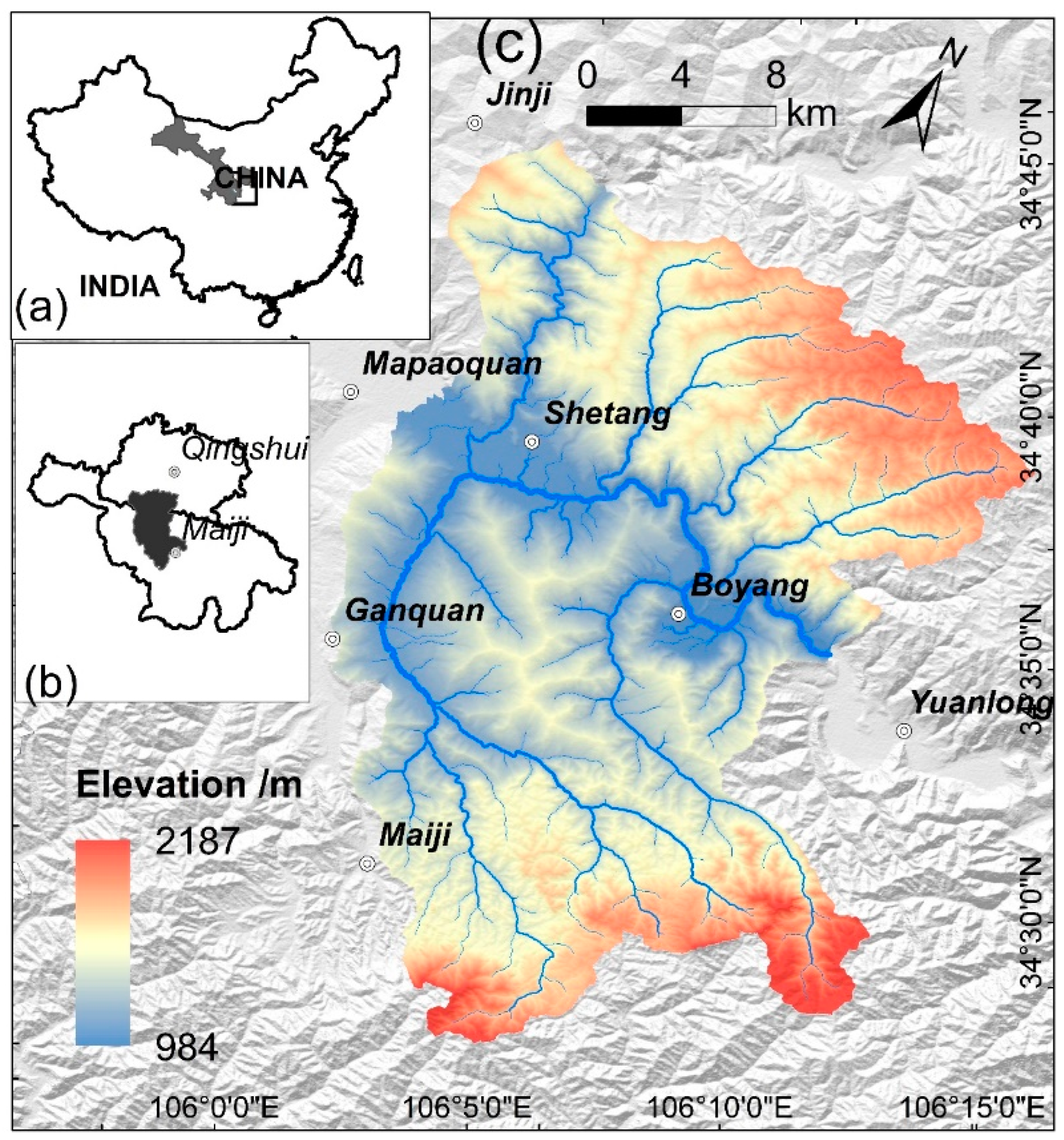
2. Study Area
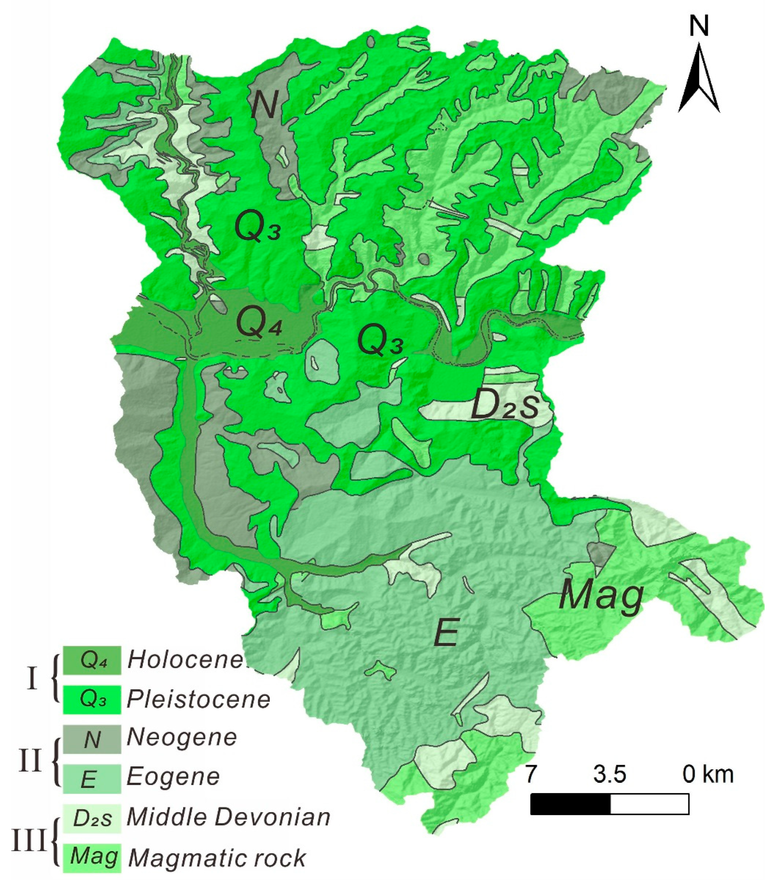
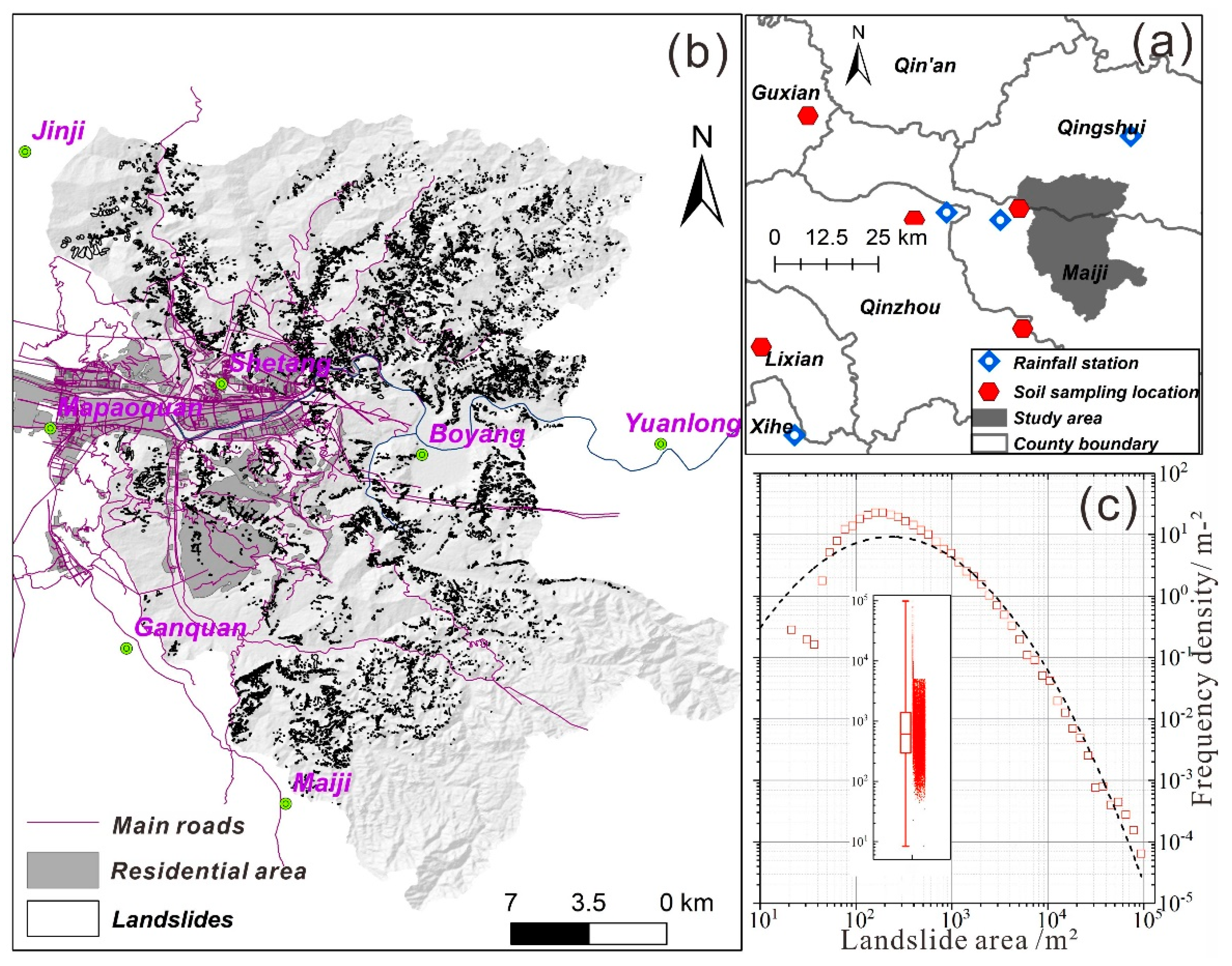
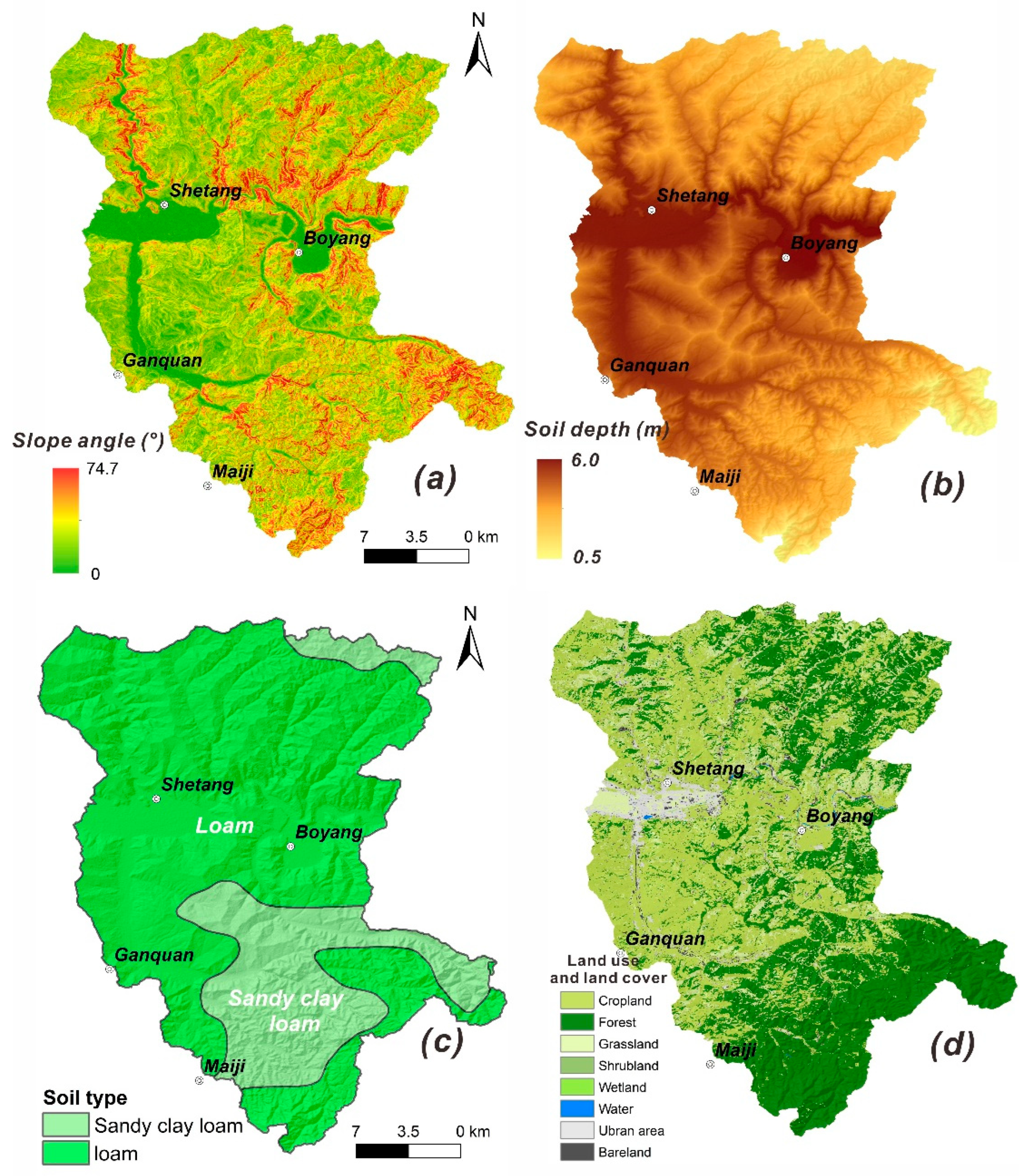
2.1. General Settings
2.2. The Landslide Inventory
3. Data and Methods
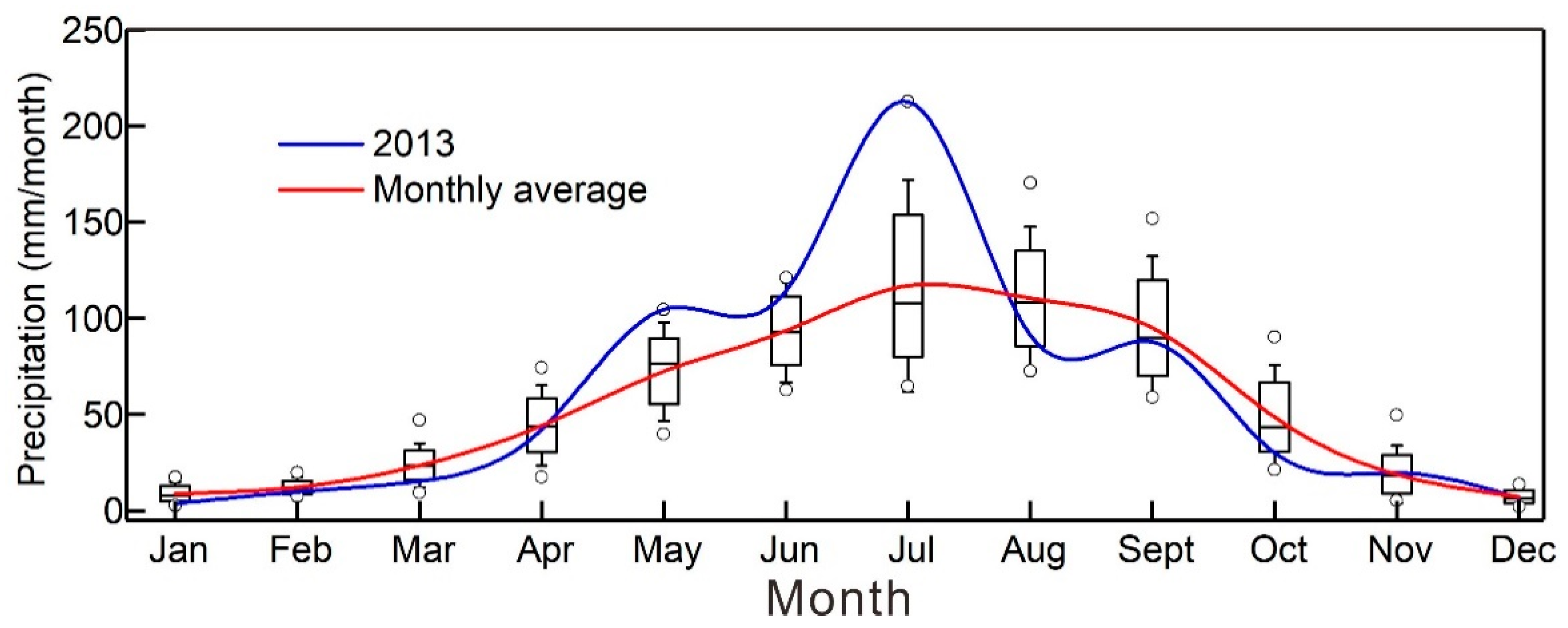
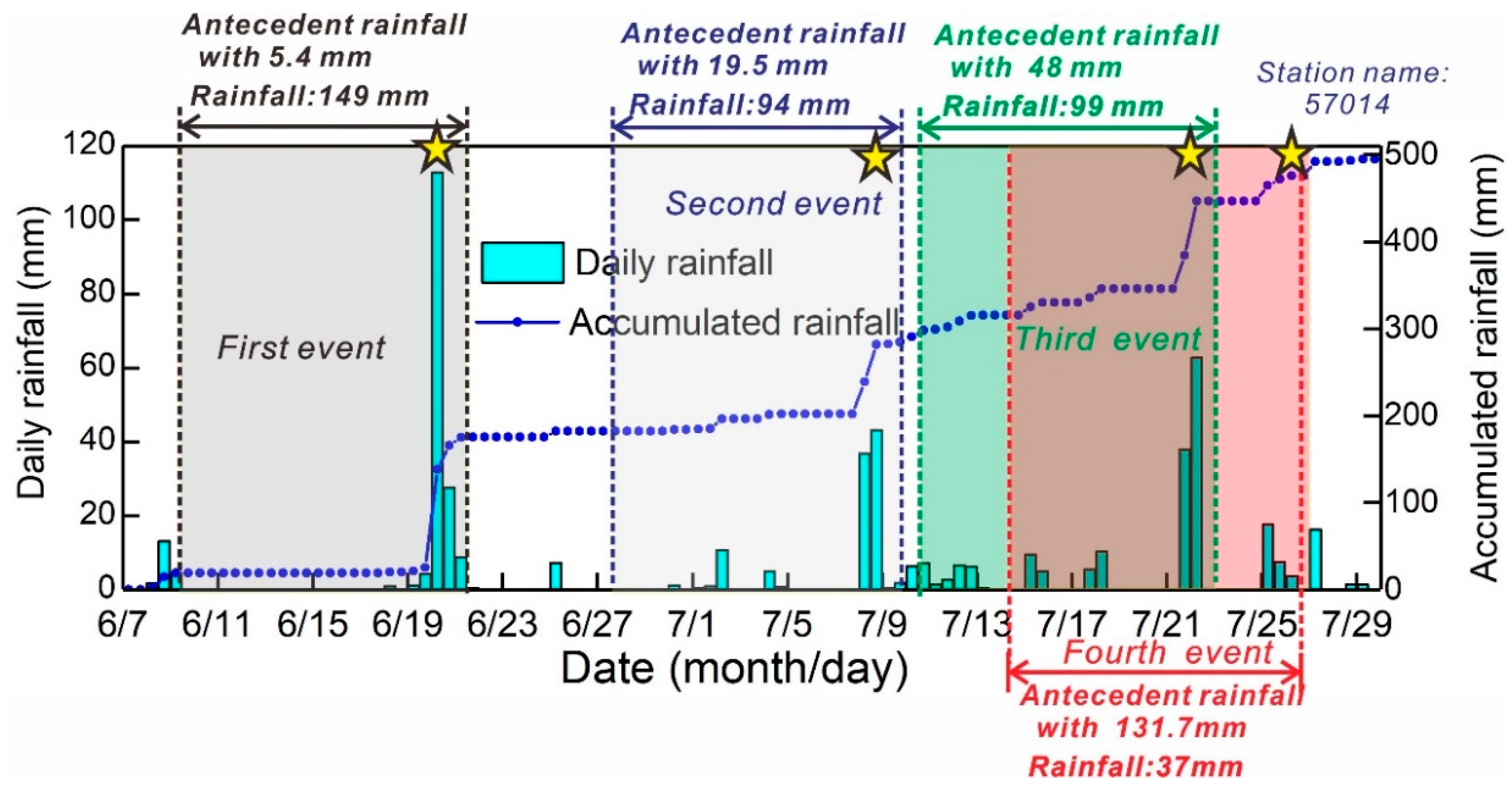
3.1. Rainfall Data
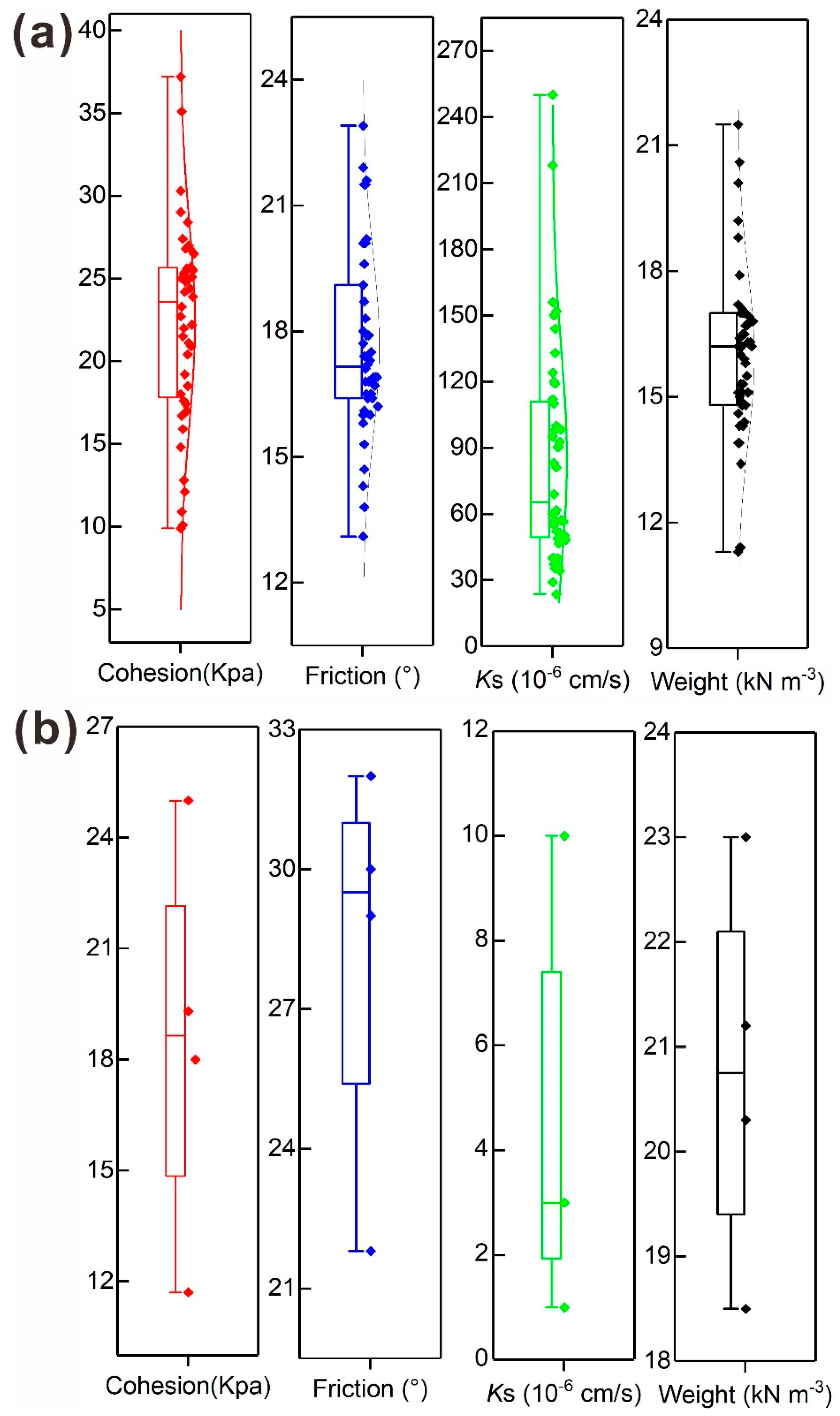
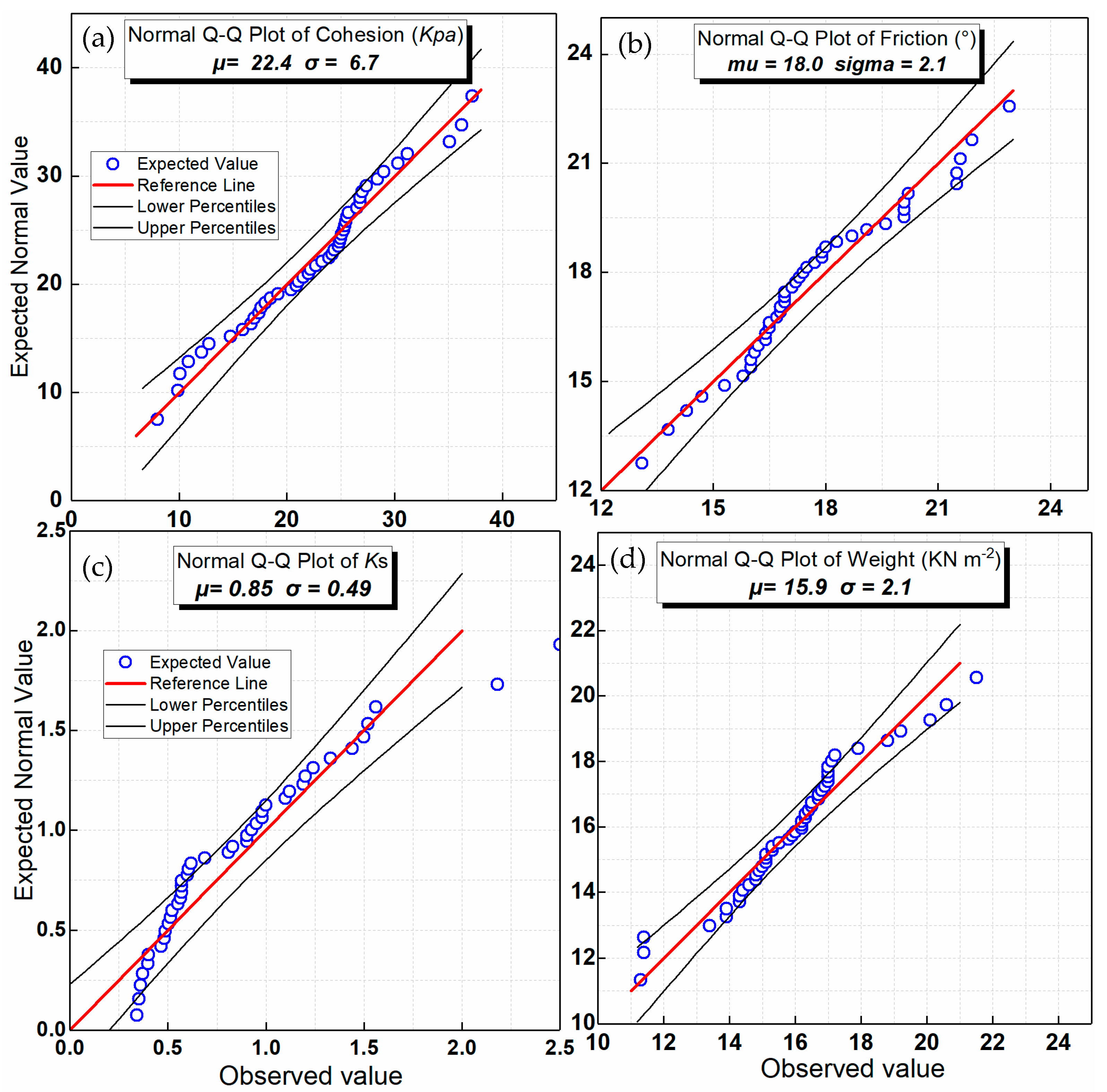
3.2. Analysis of Soil Samples
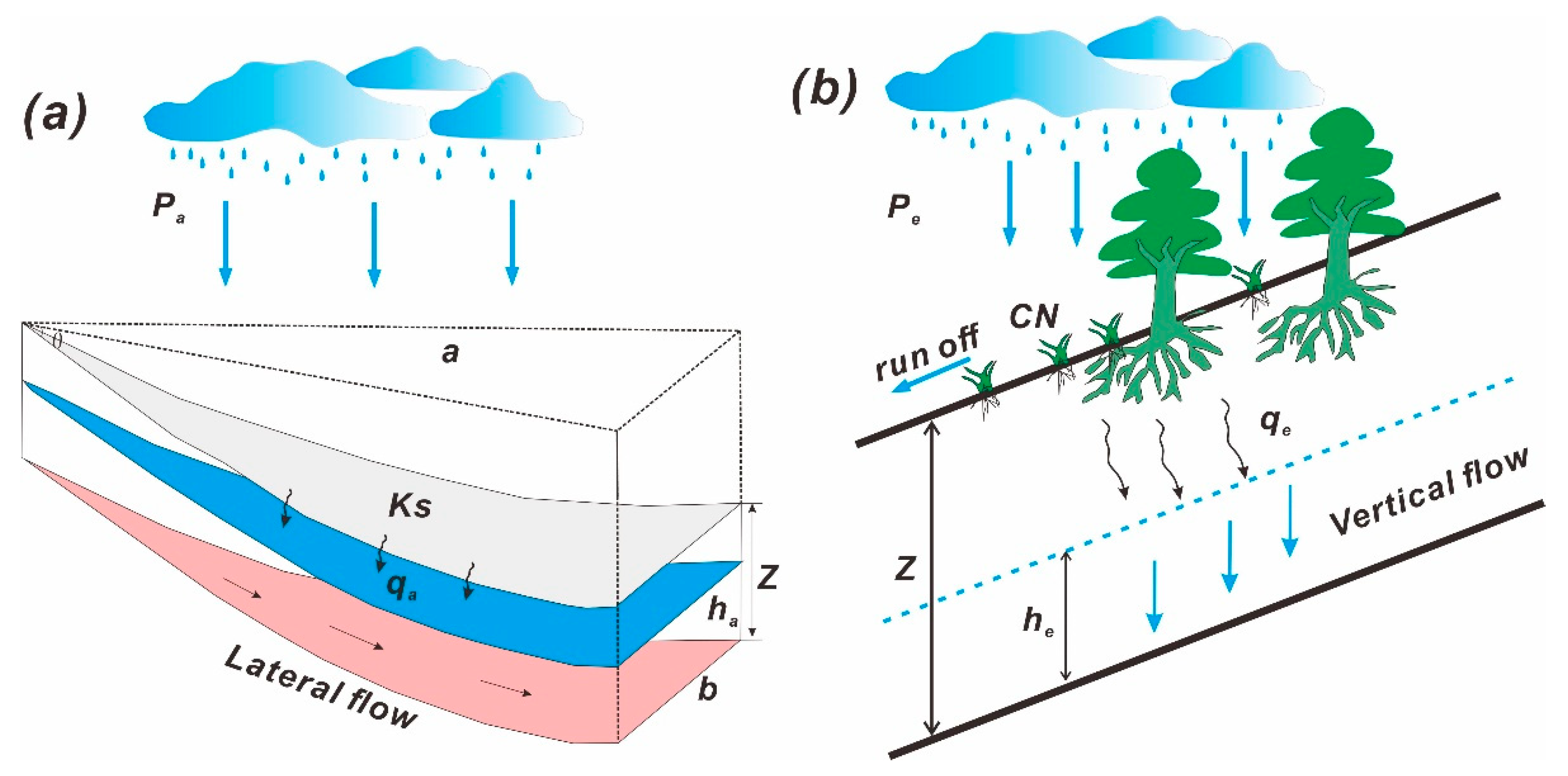
3.3. Brief Description of the FSLAM Model
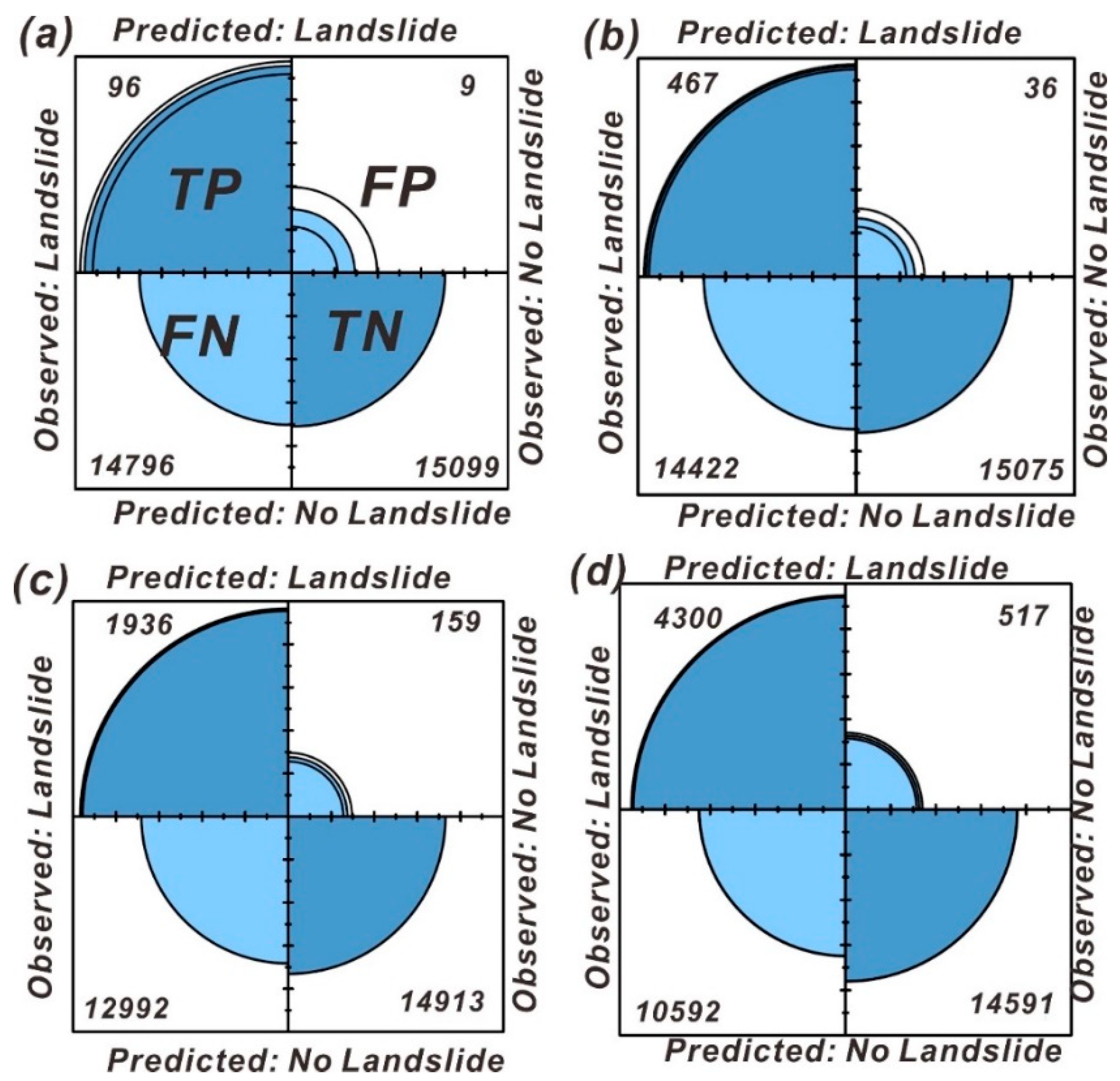
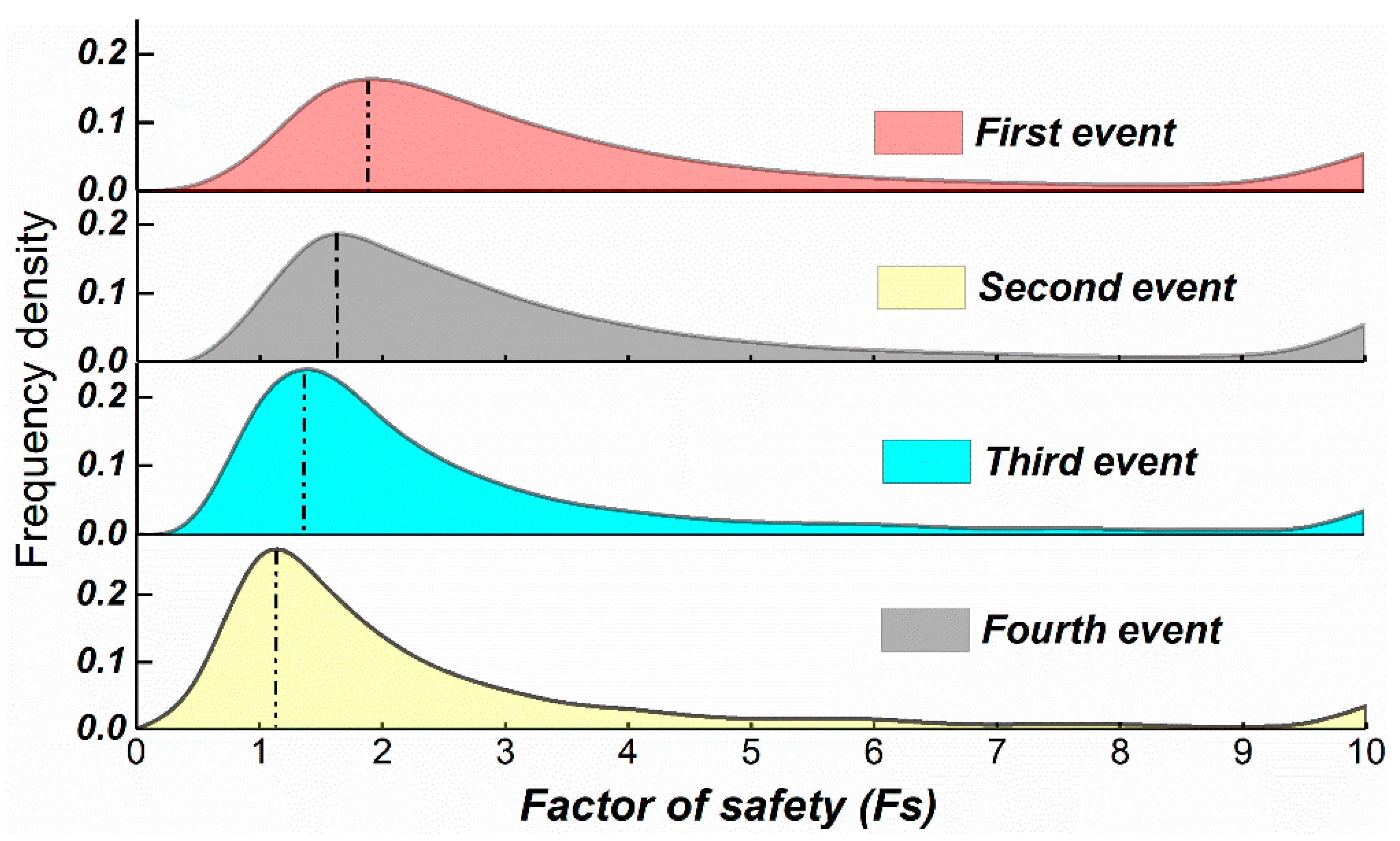
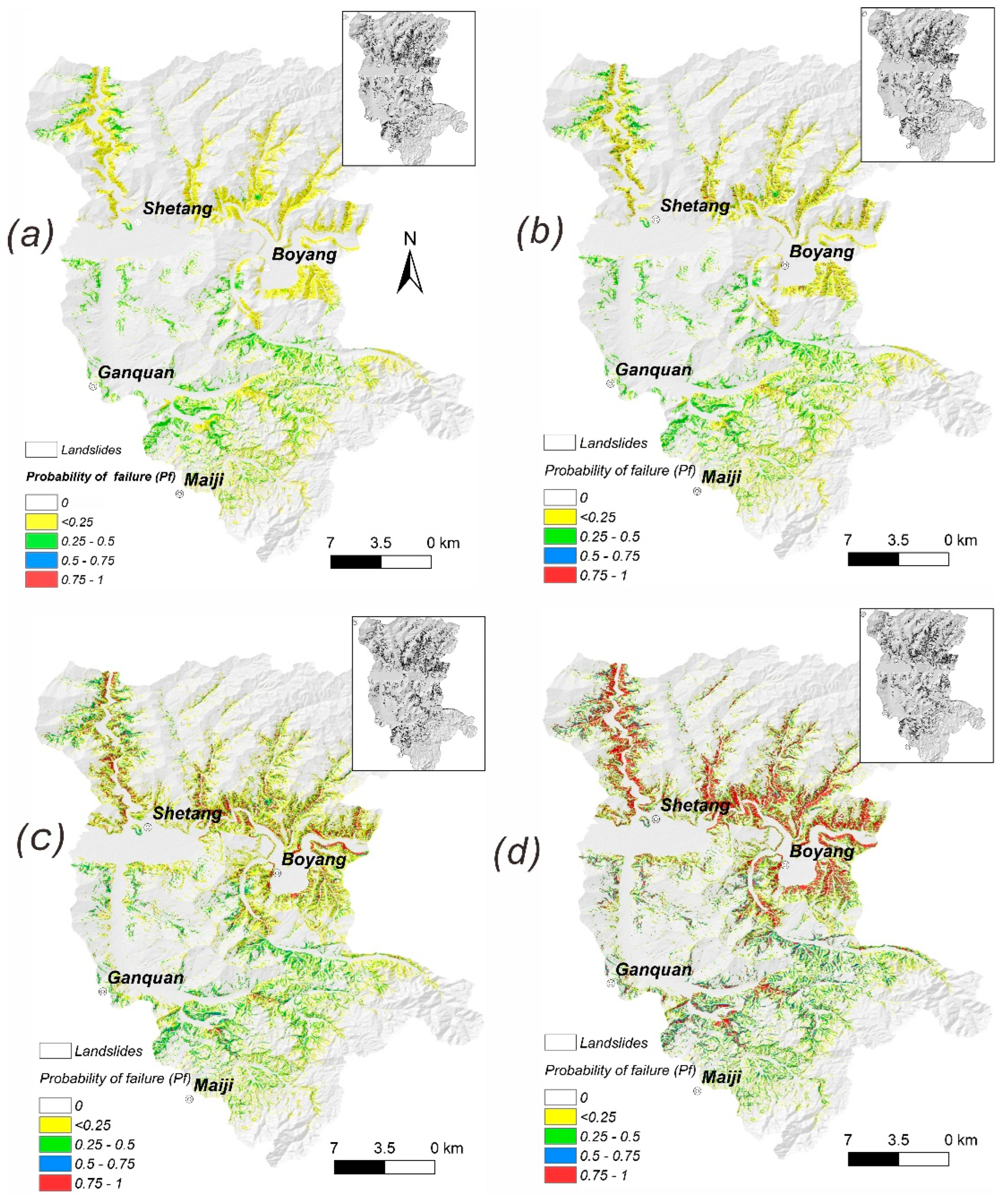
4. Result
5. Discussion
6. Conclusions
Author Contributions
Funding
Data Availability Statement
Conflicts of Interest
References
- Kirschbaum, D.; Kapnick, S.B.; Stanley, T.; Pascale, S. Changes in Extreme Precipitation and Landslides Over High Mountain Asia. Geophys. Res. Lett. 2020, 47, e2019GL085347. [Google Scholar] [CrossRef]
- Emberson, R.; Kirschbaum, D.; Stanley, T. Global connections between El Nino and landslide impacts. Nat. Commun. 2021, 12, 2262. [Google Scholar] [CrossRef] [PubMed]
- Petley, D. Global patterns of loss of life from landslides. Geology 2012, 40, 927–930. [Google Scholar] [CrossRef]
- Lin, Q.; Wang, Y. Spatial and temporal analysis of a fatal landslide inventory in China from 1950 to 2016. Landslides 2018, 15, 2357–2372. [Google Scholar] [CrossRef]
- Gariano, S.L.; Guzzetti, F. Landslides in a changing climate. Earth-Sci. Rev. 2016, 162, 227–252. [Google Scholar] [CrossRef] [Green Version]
- Guo, Z.; Chen, L.; Yin, K.; Shrestha, D.P.; Zhang, L. Quantitative risk assessment of slow-moving landslides from the viewpoint of decision-making: A case study of the Three Gorges Reservoir in China. Eng. Geol. 2020, 273, 105667. [Google Scholar] [CrossRef]
- Guzzetti, F.; Gariano, S.L.; Peruccacci, S.; Brunetti, M.T.; Marchesini, I.; Rossi, M.; Melillo, M. Geographical landslide early warning systems. Earth-Sci. Rev. 2020, 200, 102973. [Google Scholar] [CrossRef]
- Baum, R.; Godt, J. Early warning of rainfall-induced shallow landslides and debris flows in the USA. Landslides 2010, 7, 259–272. [Google Scholar] [CrossRef]
- Guzzetti, F.; Peruccacci, S.; Rossi, M.; Stark, C. The rainfall intensity-duration control of shallow landslides and debris flows: An update. Landslides 2008, 5, 3–17. [Google Scholar] [CrossRef]
- Segoni, S.; Rosi, A.; Rossi, G.; Catani, F.; Casagli, N. Analysing the relationship between rainfalls and landslides to define a mosaic of triggering thresholds for regional scale warning systems. Nat. Hazards Earth Syst. Sci. 2014, 2, 2637–2648. [Google Scholar] [CrossRef]
- Gioia, E.; Gabriella, S.; Ferretti, M.; Godt, J.; Baum, R.; Marincioni, F. Application of a process-based shallow landslide hazard model over a broad area in Central Italy. Landslides 2016, 13, 1197–1214. [Google Scholar] [CrossRef]
- Park, H.J.; Lee, J.-H.; Woo, I. Assessment of rainfall-induced shallow landslide susceptibility using a GIS-based probabilistic approach. Eng. Geol. 2013, 161, 1–15. [Google Scholar] [CrossRef]
- Xie, M.; Esaki, T.; Zhou, G. GIS-Based Probabilistic Mapping of Landslide Hazard Using a Three-Dimensional Deterministic Model. Nat. Hazards 2004, 33, 265–282. [Google Scholar] [CrossRef]
- Pourghasemi, H.R.; Rahmati, O. Prediction of the landslide susceptibility: Which algorithm, which precision? Catena 2017, 162, 177–192. [Google Scholar] [CrossRef]
- Bordoni, M.; Vivaldi, V.; Lucchelli, L.; Ciabatta, L.; Brocca, L.; Galve, J.; Meisina, C. Development of a data-driven model for spatial and temporal shallow landslide probability of occurrence at catchment scale. Landslides 2020, 18, 1209–1229. [Google Scholar] [CrossRef]
- Tanyu, B.F.; Abbaspour, A.; Alimohammadlou, Y.; Tecuci, G. Landslide susceptibility analyses using Random Forest, C4.5, and C5.0 with balanced and unbalanced datasets. Catena 2021, 203, 105355. [Google Scholar] [CrossRef]
- Baum, R.L.; Godt, J.W.; Savage, W.Z. Estimating the timing and location of shallow rainfall-induced landslides using a model for transient, unsaturated infiltration. J. Geophys. Res. F Earth Surf. 2010, 115, 126–153. [Google Scholar] [CrossRef]
- Chae, B.-G.; Park, H.J.; Catani, F.; Simoni, A.; Berti, M. Landslide prediction, monitoring and early warning: A concise review of state-of-the-art. Geosci. J. 2017, 21, 1033–1070. [Google Scholar] [CrossRef]
- Montgomery, D.R.; Dietrich, W.E.; Torres, R.; Anderson, S.P.; Heffner, J.T.; Loague, K. Hydrologic response of a steep, unchanneled valley to natural and applied rainfall. Water Resour. Res. 1997, 33, 91–109. [Google Scholar] [CrossRef]
- Dietrich, W.E.; Reiss, R.; Hsu, M.-L.; Montgomery, D.R. A process-based model for colluvial soil depth and shallow landsliding using digital elevation data. Hydrol. Process. 1995, 9, 383–400. [Google Scholar] [CrossRef]
- Pack, R.; Tarboton, D.; Goodwin, C.N. SINMAP 2.0—A Stability Index Approach to Terrain Stability Hazard Mapping, User’s Manual; Utah State University: Logan, UT, USA, 1999. [Google Scholar]
- Montrasio, L.; Valentino, R.; Losi, G.L. Rainfall-induced shallow landslides: A model for the triggering mechanism of some case studies in Northern Italy. Landslides 2009, 6, 241–251. [Google Scholar] [CrossRef]
- Montrasio, L.; Valentino, R.; Corina, A.; Rossi, L.; Rudari, R. A prototype system for space–time assessment of rainfall-induced shallow landslides in Italy. Nat. Hazards 2014, 74, 1263–1290. [Google Scholar] [CrossRef]
- Montrasio, L.; Valentino, R.; Meisina, C. Soil Saturation and Stability Analysis of a Test Site Slope Using the Shallow Landslide Instability Prediction (SLIP) Model. Geotech. Geol. Eng. 2018, 36, 2331–2342. [Google Scholar] [CrossRef]
- An, H.; Viet, T.T.; Lee, G.; Kim, Y.; Kim, M.; Noh, S.; Noh, J. Development of time-variant landslide-prediction software considering three-dimensional subsurface unsaturated flow. Environ. Model. Softw. 2016, 85, 172–183. [Google Scholar] [CrossRef]
- Tran, T.V.; Lee, G.; An, H.; Kim, M. Comparing the performance of TRIGRS and TiVaSS in spatial and temporal prediction of rainfall-induced shallow landslides. Environ. Earth Sci. 2017, 76, 315. [Google Scholar] [CrossRef]
- Escobar-Wolf, R.; Sanders, J.D.; Vishnu, C.L.; Oommen, T.; Sajinkumar, K.S. A GIS Tool for Infinite Slope Stability Analysis (GIS-TISSA). Geosci. Front. 2021, 12, 756–768. [Google Scholar] [CrossRef]
- He, X.; Hong, Y.; Vergara, H.; Zhang, K.; Kirstetter, P.-E.; Gourley, J.J.; Zhang, Y.; Qiao, G.; Liu, C. Development of a coupled hydrological-geotechnical framework for rainfall-induced landslides prediction. J. Hydrol. 2016, 543, 395–405. [Google Scholar] [CrossRef]
- Zhang, K.; Xue, X.; Hong, Y.; Gourley, J.J.; Lu, N.; Wan, Z.; Hong, Z.; Wooten, R. iCRESTRIGRS: A coupled modeling system for cascading flood–landslide disaster forecasting. Hydrol. Earth Syst. Sci. 2016, 20, 5035–5048. [Google Scholar] [CrossRef] [Green Version]
- Rossi, G.; Catani, F.; Leoni, L.; Segoni, S.; Tofani, V. HIRESSS: A physically based slope stability simulator for HPC applications. Nat. Hazards Earth Syst. Sci. 2013, 13, 151–166. [Google Scholar] [CrossRef] [Green Version]
- Tofani, V.; Bicocchi, G.; Rossi, G.; Segoni, S.; D’Ambrosio, M.; Casagli, N.; Catani, F. Soil characterization for shallow landslides modeling: A case study in the Northern Apennines (Central Italy). Landslides 2017, 14, 755–770. [Google Scholar] [CrossRef]
- Salvatici, T.; Tofani, V.; Rossi, G.; D’Ambrosio, M.; Tacconi Stefanelli, C.; Masi, E.B.; Rosi, A.; Pazzi, V.; Vannocci, P.; Petrolo, M.; et al. Application of a physically based model to forecast shallow landslides at a regional scale. Nat. Hazards Earth Syst. Sci. 2018, 18, 1919–1935. [Google Scholar] [CrossRef] [Green Version]
- Canli, E.; Mergili, M.; Thiebes, B.; Glade, T. Probabilistic landslide ensemble prediction systems: Lessons to be learned from hydrology. Nat. Hazards Earth Syst. Sci. 2018, 18, 2183–2202. [Google Scholar] [CrossRef] [Green Version]
- Cascini, L.; Ciurleo, M.; Di Nocera, S.; Gullà, G. A new–old approach for shallow landslide analysis and susceptibility zoning in fine-grained weathered soils of southern Italy. Geomorphology 2015, 241, 371–381. [Google Scholar] [CrossRef]
- De Lima Neves Seefelder, C.; Koide, S.; Mergili, M. Does parameterization influence the performance of slope stability model results? A case study in Rio de Janeiro, Brazil. Landslides 2016, 14, 1389–1401. [Google Scholar] [CrossRef] [Green Version]
- Schilirò, L.; Cevasco, A.; Esposito, C.; Mugnozza, G.S. Shallow landslide initiation on terraced slopes: Inferences from a physically based approach. Geomat. Nat. Hazards Risk 2018, 9, 295–324. [Google Scholar] [CrossRef] [Green Version]
- Salciarini, D.; Godt, J.W.; Savage, W.Z.; Conversini, P.; Baum, R.L.; Michael, J.A. Modeling regional initiation of rainfall-induced shallow landslides in the eastern Umbria Region of central Italy. Landslides 2006, 3, 181–194. [Google Scholar] [CrossRef]
- Raia, S.; Alvioli, M.; Rossi, M.; Baum, R.L.; Godt, J.; Guzzetti, F. Improving Predictive Power of Physically Based Rainfall-Induced Shallow Landslide Models: A Probabilistic Approach. Geosci. Model Dev. 2014, 7, 495. [Google Scholar] [CrossRef] [Green Version]
- Lee, J.H.; Park, H.J. Assessment of shallow landslide susceptibility using the transient infiltration flow model and GIS-based probabilistic approach. Landslides 2015, 13, 885–903. [Google Scholar] [CrossRef]
- Schilirò, L.; Esposito, C.; Scarascia Mugnozza, G. Evaluation of shallow landslide-triggering scenarios through a physically based approach: An example of application in the southern Messina area (northeastern Sicily, Italy). Nat. Hazards Earth Syst. Sci. 2015, 15, 2091–2109. [Google Scholar] [CrossRef] [Green Version]
- Xue, C.; Nie, G.; Li, H.; Wang, J. Data assimilation with an improved particle filter and its application in the TRIGRS landslide model. Nat. Hazards Earth Syst. Sci. 2018, 18, 2801–2807. [Google Scholar] [CrossRef]
- Park, H.J.; Jang, J.; Lee, J.-H. Assessment of rainfall-induced landslide susceptibility at the regional scale using a physically based model and fuzzy-based Monte Carlo simulation. Landslides 2019, 16, 695–713. [Google Scholar] [CrossRef]
- Wu, S.-J.; Hsiao, Y.-H.; Yeh, K.-C.; Yang, S.-H. A probabilistic model for evaluating the reliability of rainfall thresholds for shallow landslides based on uncertainties in rainfall characteristics and soil properties. Nat. Hazards 2017, 87, 469–513. [Google Scholar] [CrossRef]
- Salciarini, D.; Fanelli, G.; Tamagnini, C. A probabilistic model for rainfall—Induced shallow landslide prediction at the regional scale. Landslides 2017, 14, 1731–1746. [Google Scholar] [CrossRef]
- Peres, D.J.; Cancelliere, A. Estimating return period of landslide triggering by Monte Carlo simulation. J. Hydrol. 2016, 541, 256–271. [Google Scholar] [CrossRef]
- Medina, V.; Hürlimann, M.; Guo, Z.; Lloret, A.; Vaunat, J. Fast physically-based model for rainfall-induced landslide susceptibility assessment at regional scale. Catena 2021, 201, 105213. [Google Scholar] [CrossRef]
- Hürlimann, M.; Guo, Z.; Puig-Polo, C.; Medina, V. Impacts of future climate and land cover changes on landslide susceptibility: Regional scale modelling in the Val d’Aran region (Pyrenees, Spain). Landslides 2022, 19, 99–118. [Google Scholar] [CrossRef]
- Xu, Y.; Allen, M.B.; Zhang, W.; Li, W.; He, H. Landslide characteristics in the Loess Plateau, northern China. Geomorphology 2020, 359, 107150. [Google Scholar] [CrossRef]
- Qi, T.; Zhao, Y.; Meng, X.; Chen, G.; Dijkstra, T. AI-Based Susceptibility Analysis of Shallow Landslides Induced by Heavy Rainfall in Tianshui, China. Remote Sens. 2021, 13, 1819. [Google Scholar] [CrossRef]
- Saulnier, G.-M.; Beven, K.; Obled, C. Including spatially variable soil depths in TOPMODEL. J. Hydrol. 1997, 202, 158–172. [Google Scholar] [CrossRef]
- He, J.; Qiu, H.; Qu, F.; Hu, S.; Yang, D.; Shen, Y.; Zhang, Y.; Sun, H.; Cao, M. Prediction of spatiotemporal stability and rainfall threshold of shallow landslides using the TRIGRS and Scoops3D models. Catena 2021, 197, 104999. [Google Scholar] [CrossRef]
- Zhuang, J.; Peng, J.; Wang, G.; Iqbal, J.; Wang, Y.; Li, W.; Zhu, X. Prediction of rainfall-induced shallow landslides in the Loess Plateau, Yan’an, China, using the TRIGRS model. Earth Surf. Process. Landf. 2016, 42, 915–927. [Google Scholar] [CrossRef]
- Gong, P.; Liu, H.; Zhang, M.; Li, C.; Wang, J.; Huang, H.; Clinton, N.; Ji, L.; Li, W.; Bai, Y.; et al. Stable classification with limited sample: Transferring a 30-m resolution sample set collected in 2015 to mapping 10-m resolution global land cover in 2017. Sci. Bull. 2019, 64, 370–373. [Google Scholar] [CrossRef] [PubMed] [Green Version]
- USDA. Urban Hydrology for Small Watersheds, 2nd ed; Technical Release; USDA: Washington, DC, USA, 1986; Volume 55.
- Guo, Z.; Torra, O.; Hürlimann, M.; Abancó, C.; Medina, V. FSLAM: A QGIS plugin for fast regional susceptibility assessment of rainfall-induced landslides. Environ. Model. Softw. 2022, 150, 105354. [Google Scholar] [CrossRef]
- Papa, M.; Trentini, G.; Carbone, A.; Gallo, A. An integrated approach for debris flow hazard assessment—A case study on the Amalfi coast—Campania, Italy. Ital. J. Eng. Geol. Environ. 2011, 983–992. [Google Scholar] [CrossRef]
- Montgomery, D.R.; Dietrich, W.E. A physically based model for the topographic control on shallow landsliding. Water Resour. Res. 1994, 30, 1153–1171. [Google Scholar] [CrossRef]
- Sarkar, S.; Roy, A.K.; Raha, P. Deterministic approach for susceptibility assessment of shallow debris slide in the Darjeeling Himalayas, India. Catena 2016, 142, 36–46. [Google Scholar] [CrossRef]
- Bueechi, E.; Klimeš, J.; Frey, H.; Huggel, C.; Strozzi, T.; Cochachin, A. Regional-scale landslide susceptibility modelling in the Cordillera Blanca, Peru—A comparison of different approaches. Landslides 2018, 16, 395–407. [Google Scholar] [CrossRef]
- Schiliro, L.; Montrasio, L.; Scarascia Mugnozza, G. Prediction of shallow landslide occurrence: Validation of a physically-based approach through a real case study. Sci. Total. Environ. 2016, 569, 134–144. [Google Scholar] [CrossRef]
- Baum, R.L.; Savage, W.Z.; Godt, J.W. TRIGRS—A Fortran Program for Transient Rainfall Infiltration and Grid-Based Regional Slope-Stability Analysis, Version 2.0; US Geological Survey: Reston, VA, USA, 2008; p. 1159. [Google Scholar]
- Rossi, M.; Guzzetti, F.; Reichenbach, P.; Mondini, A.C.; Peruccacci, S. Optimal landslide susceptibility zonation based on multiple forecasts. Geomorphology 2010, 114, 129–142. [Google Scholar] [CrossRef]
- Jolliffe, I.T.; Stephenson, D.B. Forecast Verification: A Practitioner’s Guide in Atmospheric Science; John Wiley & Sons: Hoboken, NJ, USA, 2003. [Google Scholar]
- Godt, J.; Baum, R.L.; Savage, W.Z.; Salciarini, D.; Schulz, W.; Harp, E.L. Transient deterministic shallow landslide modeling: Requirements for susceptibility and hazard assessments in a GIS framework. Eng. Geol. 2008, 102, 214–226. [Google Scholar] [CrossRef]
- Tong, X.; Peng, J.; Zhu, X.; Ma, P.; Meng, Z. Advantage infiltration depth of rainfall in loess area. Bull. Soil Water Consevation 2017, 37, 109–113. [Google Scholar]
- Crozier, M.J. Landslides: Causes, Consequences and Environment; Croom Helm: London, UK, 1986; 245p. [Google Scholar]
- Naidu, S.; Sajinkumar, K.S.; Oommen, T.; Anuja, V.J.; Samuel, R.; Muraleedharan, C. Early warning system for shallow landslides using rainfall threshold and slope stability analysis. Geosci. Front. 2017, 9, 1871–1882. [Google Scholar] [CrossRef]
- Guo, F.; Meng, X.; Li, Z.; Xie, Z.; Chen, G.; He, Y. Characteristics and causes of assembled geohazards induced by the rainstorm on 25th July 2013 in Tianshui city, Gansu, China. Moutain Res. 2015, 33, 8. [Google Scholar]
- Huang, S.; Cui, S.; Xin, P.; Wang, T.; Liang, C. Study on rainfall threshold and spatial distribution of clustered shallow landslides in Tianshui City on July 25. J. Nat. Disasters 2021, 30, 181–190. [Google Scholar]


| LULC | min (Kpa) | Crmax (Kpa) | CN-9 | CN-10 |
|---|---|---|---|---|
| Cropland (10) | 2 | 4 | 69 | 79 |
| Forest (20) | 4 | 14 | 60 | 69 |
| Grassland (30) | 2 | 4 | 69 | 79 |
| Shrubland (40) | 3 | 6 | 65 | 76 |
| Wetland (50) | 0 | 0 | 100 | 100 |
| Water (60) | 0 | 0 | 100 | 100 |
| Urban area (80) | 0 | 1 | 92 | 96 |
| Bare land(90) | 0 | 0 | 100 | 100 |
Disclaimer/Publisher’s Note: The statements, opinions and data contained in all publications are solely those of the individual author(s) and contributor(s) and not of MDPI and/or the editor(s). MDPI and/or the editor(s) disclaim responsibility for any injury to people or property resulting from any ideas, methods, instructions or products referred to in the content. |
© 2023 by the authors. Licensee MDPI, Basel, Switzerland. This article is an open access article distributed under the terms and conditions of the Creative Commons Attribution (CC BY) license (https://creativecommons.org/licenses/by/4.0/).
Share and Cite
Ma, S.; Shao, X.; Xu, C.; Xu, Y. Insight from a Physical-Based Model for the Triggering Mechanism of Loess Landslides Induced by the 2013 Tianshui Heavy Rainfall Event. Water 2023, 15, 443. https://doi.org/10.3390/w15030443
Ma S, Shao X, Xu C, Xu Y. Insight from a Physical-Based Model for the Triggering Mechanism of Loess Landslides Induced by the 2013 Tianshui Heavy Rainfall Event. Water. 2023; 15(3):443. https://doi.org/10.3390/w15030443
Chicago/Turabian StyleMa, Siyuan, Xiaoyi Shao, Chong Xu, and Yueren Xu. 2023. "Insight from a Physical-Based Model for the Triggering Mechanism of Loess Landslides Induced by the 2013 Tianshui Heavy Rainfall Event" Water 15, no. 3: 443. https://doi.org/10.3390/w15030443