Variations in Precipitation at the Shimantan Reservoir, China

Abstract

Global warming substantially intensifies hydrologic cycles, causing increasing frequency and magnitude of catastrophic floods and droughts. Understanding the patterns and mechanisms of precipitation in historical periods is pivotal for regional disaster prevention and mitigation. Here, we analyzed the daily precipitation of six stations at the Shimantan Reservoir from 1952 to 2013 to examine precipitation characteristics at different time scales. The Mann–Kendall test, moving t-test, and Innovative Polygon Trend Analysis (IPTA) were employed to detect the trends and change points in total precipitation amount, frequency, and duration. Influences of atmospheric circulations on precipitation were then explored via cross-wavelet analysis. Our results showed increased average precipitation and decreased precipitation days annually at the Shimantan Reservoir in the past decades. Specifically, increased seasonal precipitation was only detected in summer, while precipitation days were mainly reduced in winter. There was a noticeable increasing to decreasing transition trend in precipitation from July to August, and a transition from decreasing to increasing from June to July in precipitation days. Summer rainfall was predominantly moderate and light, accompanied by shortening and highly fluctuating rainstorm durations. July exhibited the highest precipitation frequency and always experienced rainstorms. The Arctic Oscillation and East Asian summer monsoon showed positive and negative correlations, respectively, with the changes in precipitation at the Shimantan Reservoir. Our analyses provide a fine-scale portrait of precipitation patterns and mechanisms under a changing climate and benefit regional flood control and sustainable development.

1. Introduction

The global mean temperature has increased in the past decades, and it is expected to have tremendous impacts on the global and regional hydrologic cycle [1,2]. Precipitation plays a crucial role in recharging surface water and is a fundamental component of the hydrologic cycle. Due to global warming, precipitation patterns are undergoing changes [3,4]. Anomalies of precipitation can usually exacerbate and trigger occurrences of droughts or floods and cause severe impacts on both the local environment and economy [5,6,7]. Better understanding of the mechanisms and trends of precipitation is of great importance for disaster prevention and mitigation with the background of changing climate. Thus, awareness of precipitation variations in the past decades has been rising and extensive studies have been conducted in many countries and regions [8,9]. For instance, changing characteristics of precipitation have been documented for countries like the UK [10], Italy [11], Spain [12], India [4], etc. Precipitation in the USA has been proven to have increased from 1968 to 2013 [13], and mean annual precipitation on the west coast of the USA is expected to experience an increase in the future [14].

China is one of the countries which has suffered from a lot of precipitation-induced meteorological disasters and losses [15]. The increasing frequency of precipitation events has emphasized the need to investigate changes in both the spatiotemporal characteristics of precipitation amounts and precipitation patterns [16]. For example, runoff and flood are more likely to be the results of heavy precipitation events, while moderate and light precipitation usually directly infiltrate into the soil, and the decrease in moderate and light precipitation may result in droughts. Therefore, precipitation patterns and their changes in China have also garnered more attention in recent decades. Many researchers have investigated the changes in precipitation and extreme precipitation events at different space scales in China (e.g., the Yangtze River basin, Loess Plateau, Southeast China, Northwest China) [7,17,18,19]. Zhai et al. [20] have documented the distinct regional and seasonal patterns of trends in total precipitation and precipitation extremes over China from 1951 to 2000. However, precipitation across China exhibited complicated spatiotemporal patterns under the implications of summer and winter monsoon circulations as well as complex topography, since the magnitude of climate change varies with both regional and temporal scales [21,22]. For instance, many studies have suggested a growing frequency, amount, and duration of precipitation and spatial variability in their study areas [15]. However, it has been proven that the frequency of precipitation events in China decreased between 1960 and 2000 in all seasons and regions, except for northwest China [21]. Thus, it is necessary to shed light on the changes in precipitation at a regional scale, especially the heavy precipitation in the rainy season, which could induce natural disasters like floods that seriously affect the safety of social society and economic developments in a region.

The Shimantan Reservoir is a multi-functional hydraulic project in Henan Province, China, with a drainage area of 230 km². Precipitation is the major supply of runoff and water resources in the drainage basin. The upstream of the basin is always in the regional storm center and exposed to big storms. Rapid floods were common due to the big storm center and the short and steep routing path in the area. The most well-known flood occurred on 5–8 August 1975, and caused a serious dam collapse. Therefore, it is quite necessary to investigate the variation in precipitation patterns and trends at the Shimantan Reservoir to make an accurate evaluation of hazards and to mitigate negative consequences on reservoir protection, agriculture, the ecosystem, the economy, and social safety. Several studies have been conducted on precipitation variation in Henan Province [23,24].

However, unified conclusions have not been reached due to variations in the examined timescales and regions. For instance, Zhao et al. [23] reported regional differences in the extreme precipitation index within Henan Province. They found that the extreme precipitation index significantly increased in Shangqiu City and Xihua City, but decreased in the northern cities, from 1961 to 2013. Specifically, there is limited understanding of precipitation changes at the Shimantan Reservoir. Furthermore, existing studies have primarily focused on total precipitation and precipitation extremes. There is a lack of records regarding the occurrence time of rainfall events of different magnitudes and the frequency of rainfall events with varying intensities, as well as the relationship between atmospheric circulations and precipitation characteristics. These indicators have a significant impact on regional water management and disaster prevention, but they have not received enough attention.

Trend analysis is a highly effective method for observing precipitation variability. There are several methodologies available for trend analysis [25,26,27,28]. Mann-Kendall (MK) test is one of the most popular methods for analyzing trends in the precipitation [11,12,22]. For instance, Bartolini et al. [29] applied the Mann–Kendall method to annual precipitation data from 1955 to 2013 at 35 weather stations in Tuscany, Italy. Similarly, Tian et al. [30] used the Mann–Kendall method and Sen’s nonparametric method to assess the statistical significance and magnitudes of trends in temperature and precipitation extremes in China’s major grain-producing area. However, these traditional trend analysis methods have limitations. They require a certain length of data in terms of time and assume independence without any serial correlation, preventing sequential comparisons between different parts of the same data. To address these limitations, Sen [28] developed an Innovative Trend Analysis (ITA) method, which was further improved with the Innovative Polygon Trend Analysis (IPTA) in 2019 [31]. Unlike other methods, IPTA does not rely on assumptions and has gained popularity due to its ability to analyze inter-period transitions and seasonal trends across various time scales (daily, monthly, seasonal, and annual) [32]. However, the IPTA method has not been widely applied in precipitation research in China. Additionally, the large-scale ocean-atmospheric circulation patterns may have a great influence on precipitation changes [33,34]. Therefore, examining the relationship between precipitation and these circulation factors at multiple time scales can enhance our understanding and prediction of precipitation events at the Shimantan Reservoir.

To address the above research gaps, the objective of this study is to (1) identify the variability and trends in precipitation, focusing mainly on the changes in precipitation amount, precipitation days, occurrence frequency, and duration of precipitation events with different intensities from 1952–2013 at the Shimantan Reservoir with the application of the Mann–Kendall (MK) and Innovative Polygon Trend Analysis (IPTA) methods, and (2) to explore the relationship between atmospheric circulations and precipitation characteristics. The primary goal of this study is to evaluate the changing characteristics and provide a reliable basis for decision making on water resources management in the region in the context of global warming.

2. Materials and Methods

2.1. Study Area

The Shimantan Reservoir is an important hydraulic project in Henan Province, China. It was originally built in 1951, and provides multiple functions, including flood control, industrial water supply, agricultural irrigation, etc. It mainly controls the upper reaches of the Huai River, with a total drainage area of 230 km². The Shimantan Reservoir is located in Wugang City, and it belongs to a temperate continental monsoon climate, with four distinct seasons and a mild climate. The annual average temperature in the drainage basin of the Shimantan Reservoir is 16.7 °C, and the average relative humidity is 77%. The average annual precipitation in the basin above the Shimantan Reservoir was 1001.9 mm from 1956–2010. Precipitation varies greatly among years and seasons, with abundant rainfall concentrated in summer (i.e., May to September) and low precipitation occurring from October to April. The wind in the study area is always slight and gentle, and the average wind speed in the area is 3 m/s [35]. The river valley at the Shimantan Reservoir dam is narrow. The overlay layer is thin, and the rock on both banks is exposed. It is made up of quartzose sandstones with a massive structure. The terrain of the upper drainage area of the reservoir is basically high in the northwest and southeast, and low in the northeast and southwest. The southeastern and northwestern part is a low mountainous area, while the northeastern part is a hilly ridge area.

The runoff in the drainage area is mostly replenished by rainfall. Nearly 50% of the area is mountainous and covered by forests, shrubs, and weeds. Furthermore, the three major rivers in the basin, namely the Jiagang River, Shuimowan River, and Cao Bagou River, form a fan-shaped stream network. The short and steep routing path makes it more likely to experience rapid floods when heavy rainfall occurs. Due to the dam collapse in 1975 caused by the extraordinarily heavy rainfall, the dam of the reservoir was rebuilt in 1993 and commenced operation in January 1998. The rebuilt Shimantan Reservoir is designed to provide 33 million cubic meters of industrial and domestic water annually. It has provided more than 200 million cubic meters of industrial water since 1998, and produced significant irrigation benefits, with an average value of 5.77 million RMB per year. This not only satisfies the industrial and domestic water demand, but also alleviates the unreasonable water supply caused by groundwater overexploitation and other ecological environment problems.

2.2. Data Collection and Preprocessing

In this study, daily precipitation and sub-daily rainstorm data were collected from six hydrological stations at the Shimantan Reservoir from 1952 to 2013, which were provided by Tian et al. [36]. Data quality control was conducted to guarantee the accuracy of climate indices. The basic information on each hydrological station is given in

Table 1. Basic information of the selected stations.

Station Number	Station Name	Longitude	Latitude	Station Type	Data Series Length
50320350	ShimanTan	113.56	33.29	Rainfall	1952–1980 and 1994–2013
50320400	GunHeLi	113.59	33.35	Rainfall	1981–1993
50320050	ShangDian	113.45	33.23	Rainfall	1952–2013
50320100	DaoZiLing	113.55	33.18	Rainfall	1976–2013
50320150	YuanMen	113.53	33.22	Rainfall	1956–2013
50320200	BaiZhuang	113.47	33.29	Rainfall	1956–2013

. Based on the data from these six stations, regional average values of the Shimantan Reservoir were then obtained by applying the arithmetic average method.

When processing precipitation data, a day with a daily precipitation of more than 0.1 mm is considered as a precipitation day. Precipitation amount and precipitation days are calculated for different time scales (i.e., annual, seasonal, and monthly) based on the daily precipitation data. According to the climatic characteristics of the Shimantan Reservoir basin, a year is divided into four seasons: spring, summer, autumn, and winter. Spring consists of the months of March, April, and May. Summer comprises June, July, and August. Autumn encompasses September, October, and November. December, January, and February of the following year are winter months.

The observed precipitation data were then parsed into a series of discrete events by applying an interevent time definition (IETD) [37]. In this study, 5 h was selected as the interevent time (IET) to separate the precipitation events according to the characteristics of frequent summer precipitation at the Shimantan Reservoir. This means that if the duration of a non-precipitation period between two adjacent precipitation events was longer than 5 h, then these two precipitation events were defined as two individual ones. The precipitation events were subsequently classified into four categories (i.e., light rain, moderate rain, heavy rain, and rainstorm) according to the amount of precipitation in each event. The specific standard of the classification is listed in

Table 2. Classification of precipitation events according to precipitation amount.

Categories	Light Rain	Moderate Rain	Heavy Rain	Rainstorm
Precipitation amount during an event	≤10 mm	10–25 mm	25–50 mm	≥50 mm

.

Furthermore, the intensity of rainfall is classified into four grades (i.e., >2 mm/h, 2–4 mm/h, 4–8 mm/h, and >8 mm/h) according to the basic characteristics of precipitation at the Shimantan Reservoir. Detailed classification criteria are shown in

Table 3. Classification criteria of rainfall intensity.

Categories	Low Intensity	Medium Intensity	High Intensity	Extreme Intensity
Rainfall intensity	<2 mm/h	2–4 mm/h	4–8 mm/h	>8 mm/h

. The number of occurrences of precipitation events achieving each intensity level was also calculated.

2.3. Variability and Trends in Precipitation

To identify the variability and trends in precipitation at the Shimantan Reservoir, the propensity rate and Mann–Kendall test were first employed to ascertain the changing trends in the variables, including precipitation amount, precipitation days, occurrence frequency, and duration of precipitation events with different intensities. Then, the moving t-test was applied to determine the mutation year of each precipitation variable.

2.3.1. Propensity Rate

The propensity rate is a widely used coefficient in climate change studies. To obtain the propensity rate, a linear regression equation of each precipitation variable (e.g., precipitation amount, occurrences of different precipitation events…) versus time was conducted in this study as follows:

$$y_i=b{x}_i+b_0$$

(1)

where y_i is the precipitation variable selected in this study (i.e., precipitation amount, precipitation days, rainstorm duration, rainstorm frequency), and x_i is the year during the study period. The linear regression coefficient b is the propensity rate of the corresponding precipitation variable, and m = b × 10 is also used in some studies to represent the climate propensity rate per decade (i.e., 10 years). When b is larger than 0, it indicates that the precipitation variable series is showing an upward trend, and vice versa.

2.3.2. Mann–Kendall Trend Test

The Mann–Kendall test is a non-parametric test proposed by Mann and Kendall [25,27,38]. Since it was recommended by the World Meteorological Organization (WMO), the Mann-Kendall test has been applied by many researchers to analyze the changing trends and abrupt changes in time-series factors such as runoff, temperature, precipitation, and water quality [39,40]. The Mann–Kendall test does not require samples to obey a prescribed distribution and is not disturbed by outliers in the series. Hence, it is always able to accurately detect trends in the time series [41]. In addition, its calculation process is much simpler than other tests, which makes it, currently, a commonly used method for detecting trends [42].

In the Mann–Kendall test, it is assumed that data of each precipitation variable X are treated as a series of independent random variables [x₁, x₂, ……, x_n] with the same distribution pattern. Its statistically empirical formula is listed below:

$$S={\displaystyle \sum _{i=1}^{n-1}{\displaystyle \sum _{k=i+1}^n\mathrm{sgn}(x_k-x_i)}}$$

(2)

where x_k and x_i are the sample values of each precipitation variable (i.e., precipitation amount, precipitation days, rainstorm duration, rainstorm frequency) corresponding to year k and year i, and n is the length of the data series. And,

$$\mathrm{sgn}(\theta )=\left\{\begin{array}{c}1\\ 0\\ -1\end{array}\right.\begin{array}{c}\\ \\ \end{array}\begin{array}{c}\theta >0\\ \theta =0\\ \theta <0\end{array}$$

(3)

In addition, when the sample size of the data series is larger than 10, the distribution of the statistic S is close to a normal distribution. Then:

$$Z=\left\{\begin{array}{c}\frac{S-1}{\sqrt{\mathrm{var}(S)}},S>0\\ 0,S=0\\ \frac{S+1}{\sqrt{\mathrm{var}(S)}},S<0\end{array}\right.$$

(4)

$$\mathbf{var}(s)=\frac{[n(n-1)(2n+5)-{\displaystyle {\sum }_{t}t(t-1)(2t+5)}]}{18}$$

(5)

where n is the sample size, $t$ is the width of the ‘knot’, and ${\displaystyle \sum }$ is the total number of all ‘knot’s.

This trend is considered statistically significant at 95% when $Z {>\mathrm{Z}}_{\left(1-\alpha /2\right)}$. Where Z is the statistical value corresponding to a standard normal distribution with a median value of $1-\alpha /2$, $Z>0$ indicates an upward trend in the time series, while $Z<0$ indicates a downward trend.

2.3.3. Moving t-test

The moving t-test is one of the commonly used methods for detecting climate anomalies in a series of precipitation variables with a total sample size of n. To perform this test, a reference point is manually set for the data series of precipitation variable (X), and two sub-sequences (X₁ and X₂) of the precipitation variable are obtained. X₁ represents the data before the reference point, while X₂ represents the data after the reference point. The lengths of these sub-sequences are n₁ and n₂, respectively. By performing successive sliding calculations on these sub-sequences, a statistical sequence t can be obtained. A critical value t_α can be determined based on a given significance level α. If the absolute value of t is less than t_α, it indicates that there is no significant difference between the mean values of the precipitation variable before (X₁) and after the reference point (X₂). On the other hand, if |t| is greater than t_α, it suggests that the reference point marks an abrupt change in the entire data series of the precipitation variable. t is calculated as [41]:

$$t=\frac{\overline{x_1}-\overline{x_2}}{s\sqrt{\frac{1}{n_1}+\frac{1}{n_2}}}$$

(6)

where $s=\sqrt{\frac{n_1{s}_1{}^2+n_2{s}_2{}^2}{n_1+n_2-2}}$, s₁, and s₂ are the standard deviations of the two sub-sequences of the precipitation variable, respectively.

2.3.4. Innovative Polygon Trend Analysis

The Innovative Polygon Trend Analysis (IPTA) graphic method is an improved version of the Innovative Trend Analysis (ITA) method proposed by Şen et al. [31]. IPTA can be applied to different time scales, such as daily, monthly, seasonal, and annual scales, and considers inter-period transitions and seasonal changes. It effectively displays the trend size and slope between consecutive points, facilitating better numerical interpretation and trend derivation.

In this study, IPTA was applied to analyze monthly precipitation and monthly precipitation days data. The data for monthly precipitation and precipitation days were organized in a rectangular matrix format. Each row of the matrix represents the amount of precipitation or precipitation days for each month of the year, denoted as X_1,n, X_2,n, …, X_i,n, where i represents the month, and n represents the year. The matrix can be divided into two halves: the upper (first) part and the lower (second) part. The upper part corresponds to the indicator j as j = 1, 2, …, n/2, and the lower part corresponds to j = n/2 + 1, n/2 + 2, … n. The mean value and standard deviation of the upper and lower parts of the matrix are then calculated to obtain the mean value and standard deviation of these two series. The Cartesian coordinate system, as shown in Figure 1, is used to plot the average value (or standard deviation) of the upper series on the horizontal axis and the lower series on the vertical axis. This results in 12 points representing the values for the 12 months.

Figure 1 includes a 1:1 (45°) line. Points above the line indicate an increasing trend, while points below the line indicate a decreasing trend.

Straight lines can be drawn to connect the points of consecutive months, forming a dodecagon with varying side lengths and slopes. These lines represent the changes from one month to another. By obtaining the coordinates of each continuous scattering point on the IPTA template, the slope and length of the line between consecutive months, which are recorded as trend slope and trend length, respectively, can be calculated.

$$\left|AB\right|=\sqrt{{(x_2-x_1)}^2+{(y_2-y_1)}^2}$$

(7)

$$s=\frac{y_2-y_1}{x_2-x_1}$$

(8)

where s represents the trend slope, |AB| represents the trend length, x₁ and x₂ are values of two consecutive months in the first part in the horizontal axis, y₁ and y₂ are values of two consecutive months in the second part, respectively.

A larger trend length indicates a greater change value in the adjacent month series, while a trend slope deviating from 1 signifies a more significant change trend in the adjacent month.

The analysis of the polygon reveals that its area and shape are closely related to the precipitation conditions of the study area. If all the slopes of the lines in the IPTA template are similar, the resulting polygon will be narrow, indicating highly uniform and isotropic behavior of precipitation/precipitation days. On the other hand, wider polygons represent uneven temporal changes [31].

2.4. Relationship between Atmospheric Circulations and Precipitation Characteristics

In this study, we used cross-wavelet analysis to figure out the relationships between precipitation variables and atmospheric circulation indices. Cross-wavelet analysis is a method for exploring the multi-scale correlation between two time series [43]. Its wave spectrum shows the distribution pattern of energy resonance and covariance of the two time series, from which the correlation and consistency of the two time series at various time scales can be analyzed [44]. For two signal elements with finite energy, i.e., precipitation variable X(t) and atmospheric circulation index Y(t), their cross-wavelet transform is [43,45]:

$$W_n^{XY}(t)=W_n^X(t)\times W_n^Y{(t)}^{*}$$

(9)

where $W_n^{XY}\left(t\right)$ is the cross-wavelet transform matrix of precipitation variable series X(t) and atmospheric circulation index series Y(t). $W_n^X\left(t\right)$ and $W_n^Y\left(t\right)$ are the wavelet transformations of X(t) and Y(t), respectively. $W_n^Y\left(t\right)$* denotes the complex conjugate of $W_n^Y\left(t\right)$. In this study, tests for cross-wavelet power spectra at different significance levels were conducted with a red normalized noise power spectrum.

In addition, the complex angle of $W_n^{XY}\left(t\right)$ was used to represent the relative phase relationship between the time series of precipitation variable X(t) and the atmospheric circulation index Y(t). Based on the relationship between phase angle and period, the length of time for phase lag or advance can be calculated. For areas with statistical significance greater than 5% and outside the influence cone, this article uses the cyclic average of phases to quantify phase relationships. By estimating the average value and confidence interval of the phase difference, the phase difference at the meeting point between each scale component of two time series is calculated, achieving a quantitative representation of the phase relationship between X(t) and Y(t). In areas with a confidence level greater than 95%, the circular average phase angle is used to represent it. There are $i$ angles $q_i$ ($i=1,..., n$), and the average sample value of angle $q_i$ is denoted as $q$, hereinafter referred to as the average angle. The calculation formula is [46]:

$$q=\arg (x,y)$$

(10)

$$x={\displaystyle {\sum }_{i=1}^n{\cos q}_i}$$

(11)

$$y={\displaystyle {\sum }_{i=1}^n{\sin x}_i}$$

(12)

The direction of the wavelet phase angle arrow can determine the phase relationship between two time series at the corresponding time and scale. When the cross-wavelet correlation coefficient of two time series is high, the degree of advance (lag) of the latter sequence relative to the previous sequence can be estimated by the angle between the wavelet phase angle arrow direction and the time axis.

3. Results and Discussion

3.1. Variation in Annual Precipitation Characteristics at the Shimantan Reservoir

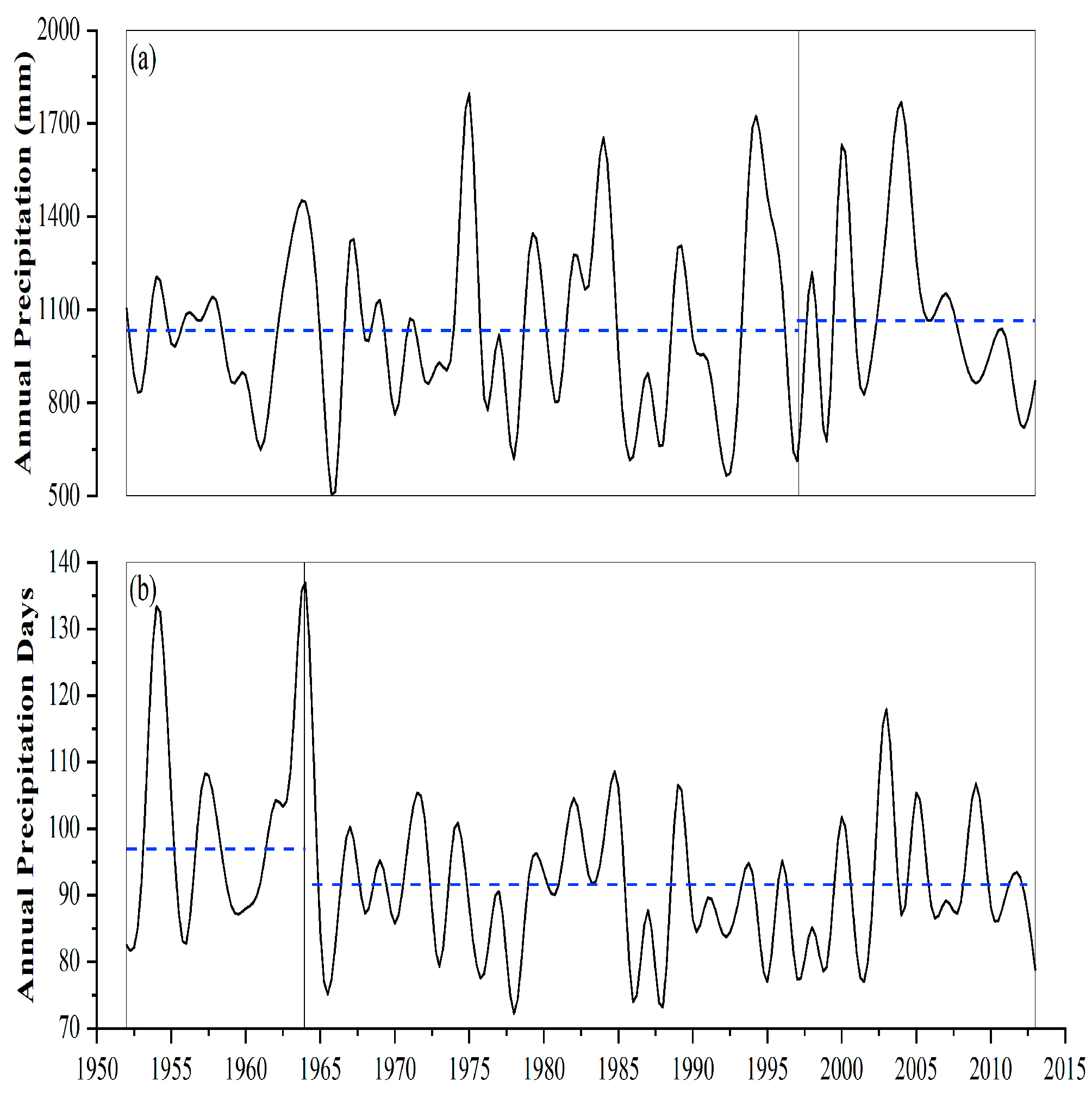
The changes in annual precipitation at the Shimantan Reservoir are shown in Figure 2. It can be seen that annual precipitation at the Shimantan Reservoir has undergone a pronounced fluctuation from 1952 to 2013, with a maximum value of 1796 mm in 1975 and a minimum value of 512 mm in 1966 (Figure 2a). Overall, there were no statistically significant trends in annual precipitation and annual precipitation days (Z = 0.011 < 1.96). The average annual precipitation and annual precipitation days during our study period were 1049 mm and 93 days, respectively. Based on the results of the moving t-test, the abrupt decreasing point of annual precipitation days happened in 1964, while a slight increasing point in annual precipitation was observed in the year 1996.

3.2. Intra-Annual Distribution and Variation in Precipitation at the Shimantan Reservoir

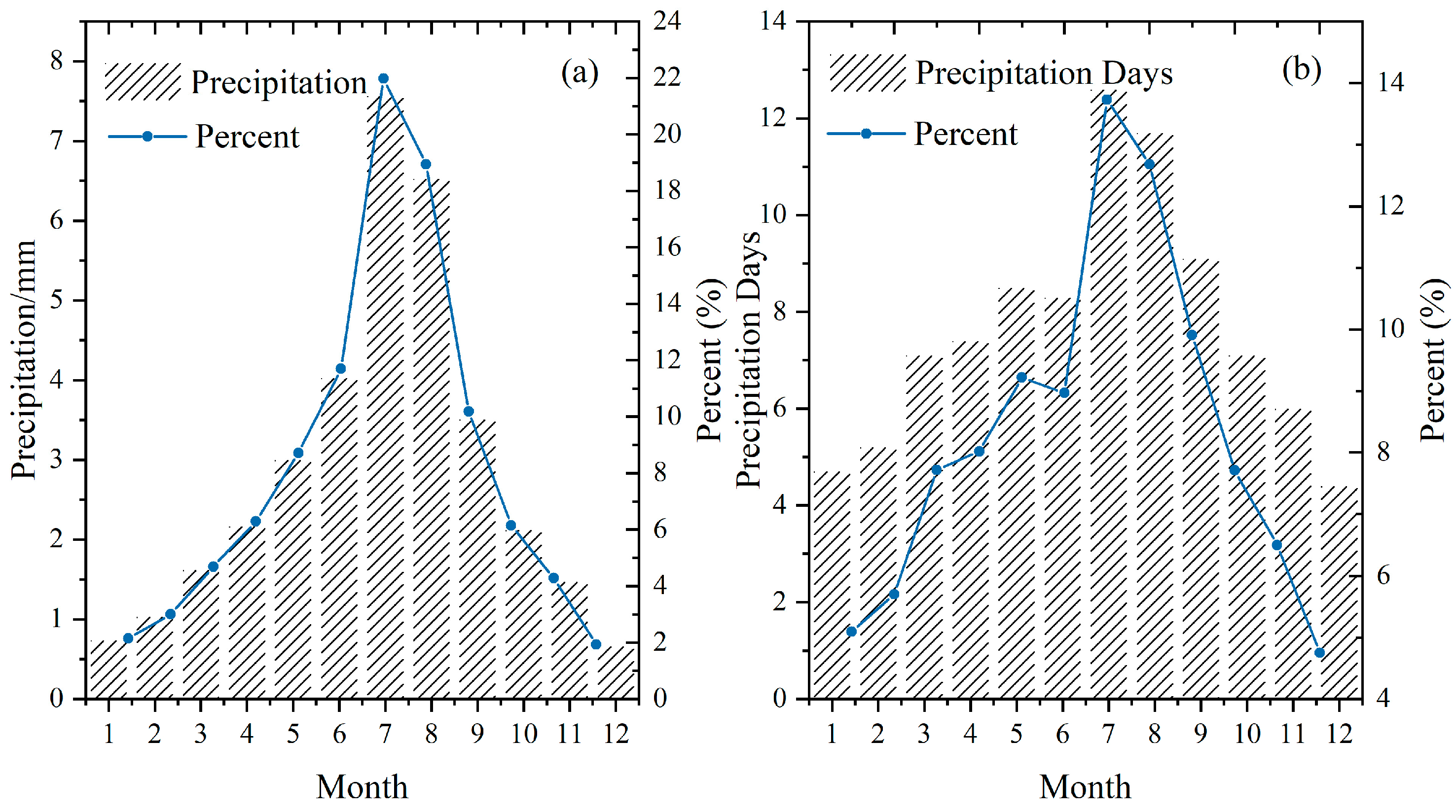
Monthly variation in precipitation amount and precipitation days at the Shimantan Reservoir is illustrated in Figure 3. As shown in the figure, precipitation at the Shimantan Reservoir was not uniformly distributed in the year (Figure 3a). The precipitation in the rainy season (i.e., April to October) accounted for 83.96% of the annual amount, of which about 40.9% was concentrated in July and August. Nearly 22 percent of the total precipitation was produced in July, whereas little precipitation occurred in the dry seasons; for example, only 1.93% of the annual precipitation was found in December (Figure 3a). Figure 3b shows that precipitation days at the Shimantan Reservoir varied during the year. The distribution of precipitation days throughout the year was relatively uniform compared to the distribution of the precipitation amount. However, there was still some unevenness in the distribution of precipitation days. The highest number of precipitation days was observed in July, accounting for 13.73% of the total days, while December had the fewest precipitation days. In general, July and August experienced significantly more precipitation days compared to other months.

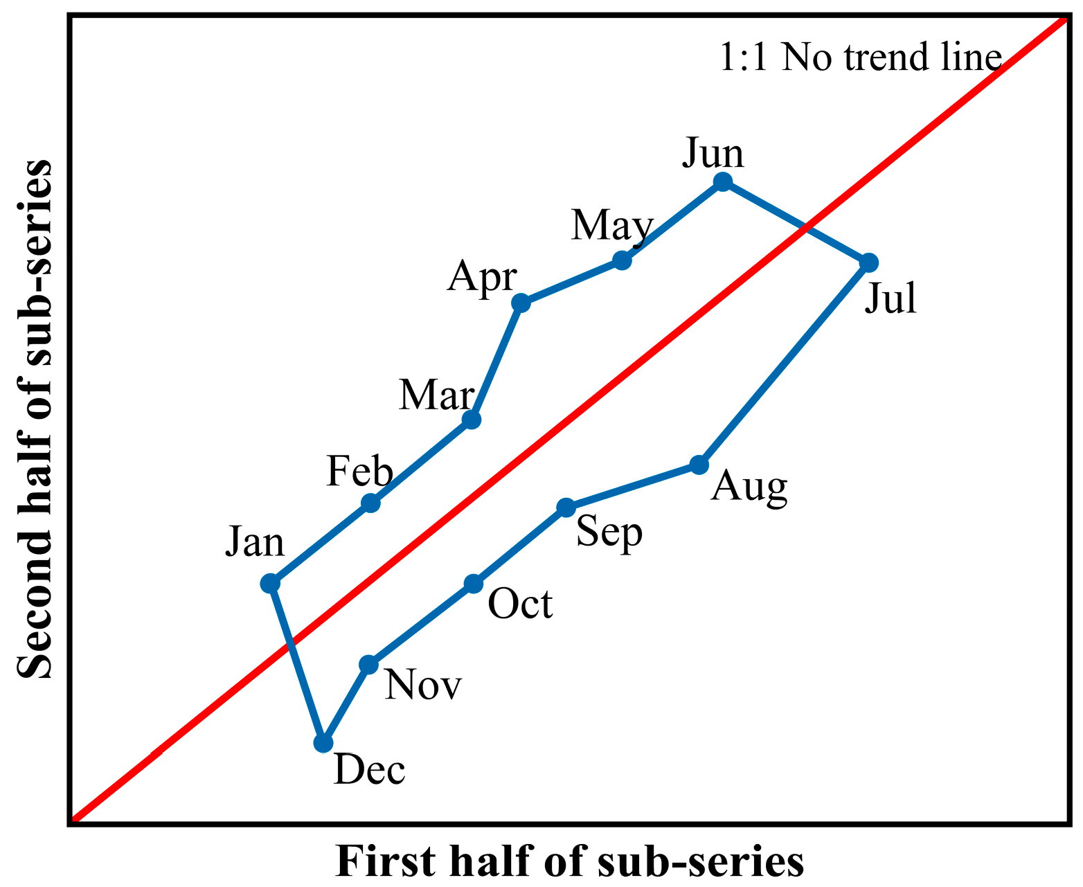
Based on the arithmetic mean graph of precipitation, precipitation in May, June, and July shows an increasing trend, while precipitation in the other months exhibits a decreasing trend (Figure 4). Notably, there is a significant surge in precipitation values during July. Additionally, there is a distinct shift from the increasing trend zone to the decreasing trend zone from July to August, and a transition from a decreasing trend to an increasing trend from April to May. The standard deviation graph also displays sharp transitions. Particularly, there are notable shifts from an increasing trend area to a decreasing trend area from July to August and October to November.

According to

Table 4. Innovative Polygon Trend Analysis (IPTA) statistical values of arithmetic mean and standard deviation for monthly precipitation and precipitation days at the Shimantan Reservoir, China.

Months	Precipitation				Precipitation Days
	Arithmetic Mean		Standard Deviation		Arithmetic Mean		Standard Deviation
	Trend Length (mm)	Trend Slope	Trend Length (mm)	Trend Slope	Trend Length (d)	Trend Slope	Trend Length (d)	Trend Slope
Jan–Feb	7.33	0.20	0.19	−0.27	0.86	1.39	0.49	0.49
Feb–Mar	28.28	0.94	0.24	0.95	2.51	0.92	0.51	−1.00
Mar–Apr	21.79	0.44	0.73	0.24	1.36	−0.45	1.15	−1.60
Apr–May	51.67	3.88	1.21	5.10	2.01	414.67	0.27	7.16
May–Jun	42.44	1.37	1.50	0.88	0.52	−8.21	0.24	−1.83
Jun–Jul	173.41	1.41	1.75	2.73	6.21	1.22	0.80	−1.53
Jul–Aug	116.56	−10.73	2.75	0.09	1.33	0.83	1.79	0.38
Aug–Sep	131.14	0.55	4.04	0.61	3.69	1.12	0.55	−1.17
Sep–Oct	60.72	1.41	1.63	0.56	2.88	2.11	0.94	0.64
Oct–Nov	24.10	0.32	1.09	−9.18	1.42	0.89	0.41	−0.05
Nov–Dec	34.29	0.80	1.06	0.41	2.36	0.68	0.36	0.26
Dec–Jan	3.64	1.04	0.04	1.11	0.37	0.90	0.37	0.95

, the trend lengths ranged from 3.64 to 173.41 mm and 0.04 to 4.04 for the arithmetic mean and standard deviation graphs of precipitation, respectively. In terms of the arithmetic mean of precipitation, the maximum trend length of 173.41 mm was observed from June–July at the Shimantan Reservoir. For the standard deviation of precipitation, the maximum trend length of 4.04 was observed from August–September. The trend slope of the mean and standard deviation for precipitation at the Shimantan Reservoir varied from −10.73 to 3.88 and from −9.18 to 5.10, respectively. Both the mean and standard deviation graphs demonstrate the presence of multiple and irregular cycles, as well as sharp decays between months, indicating complex, inhomogeneous, and chaotic precipitation behavior in the Shimantan Reservoir region.

Figure 4 shows that the minimum mean value of monthly precipitation days is in December, while the maximum is in July. From July to December, there is a relatively stable decreasing trend in the mean value of monthly precipitation days. However, there is no obvious pattern observed from December to July. The mean monthly precipitation days in July, August, and September show an increasing trend, while the mean monthly precipitation days in other months show a decreasing trend (except for February and May). April, October, and November exhibit a strong downward trend in the mean value of monthly precipitation days, with values significantly deviating from the no-trend line (45°). The arithmetic mean value graph of monthly precipitation days (Figure 4) shows two transitions. One transition is observed from a decreasing trend area to an increasing trend area from June to July. Another transition occurs from an increasing trend area to a decreasing trend area from September to October. By analyzing the standard deviation graph of monthly precipitation days (Figure 4), it can be determined that only March is in the increasing trend area, while all other months are in the decreasing trend area. Table 2 demonstrates that the maximum values of trend lengths are calculated as 6.2 days (June to July) and 1.8 days (July to August) for the mean and standard deviation, respectively. Regarding the maximum values of the trend slope, the mean value and standard deviation of monthly precipitation days have the greatest values from April to May, with trend slopes of 414.67 and 7.16, respectively.

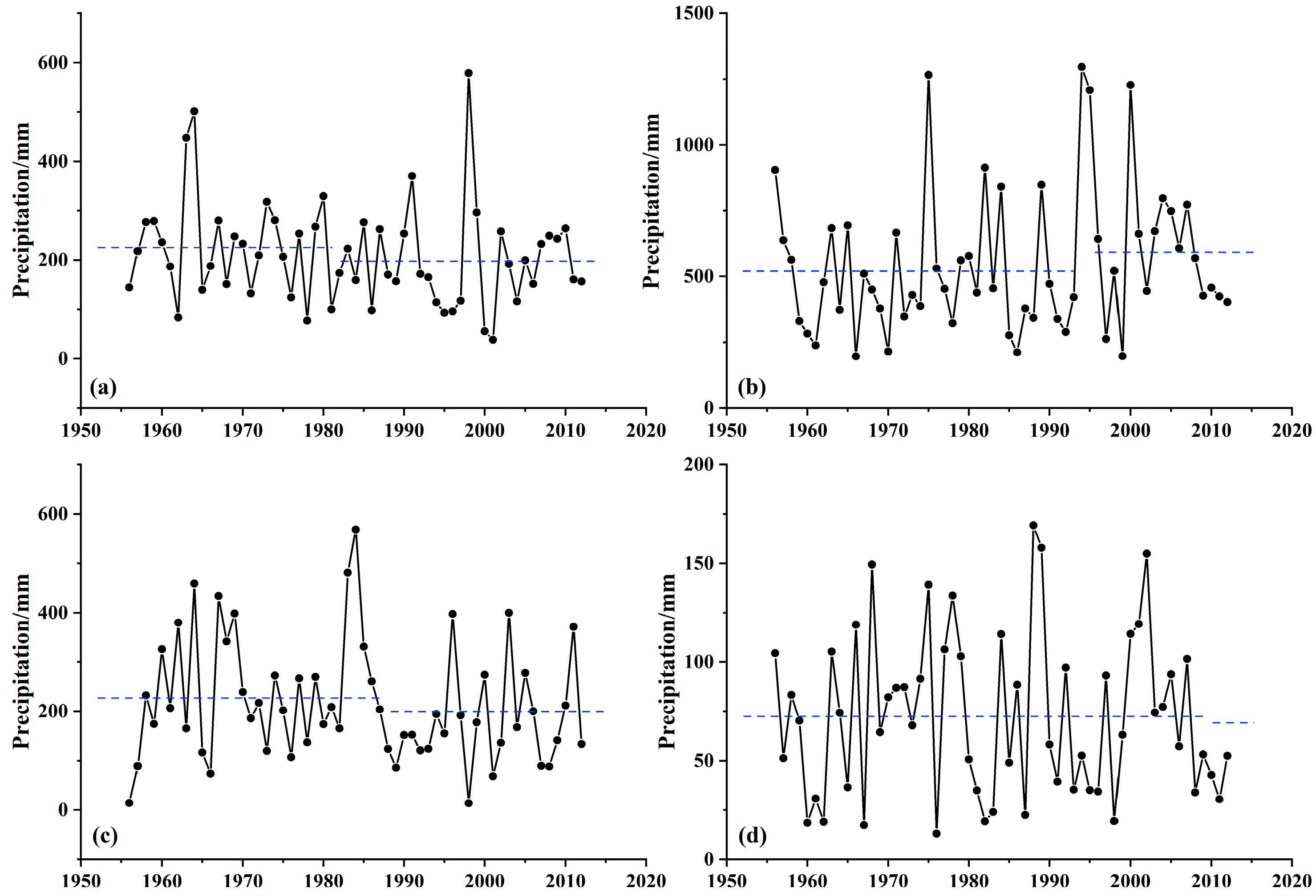
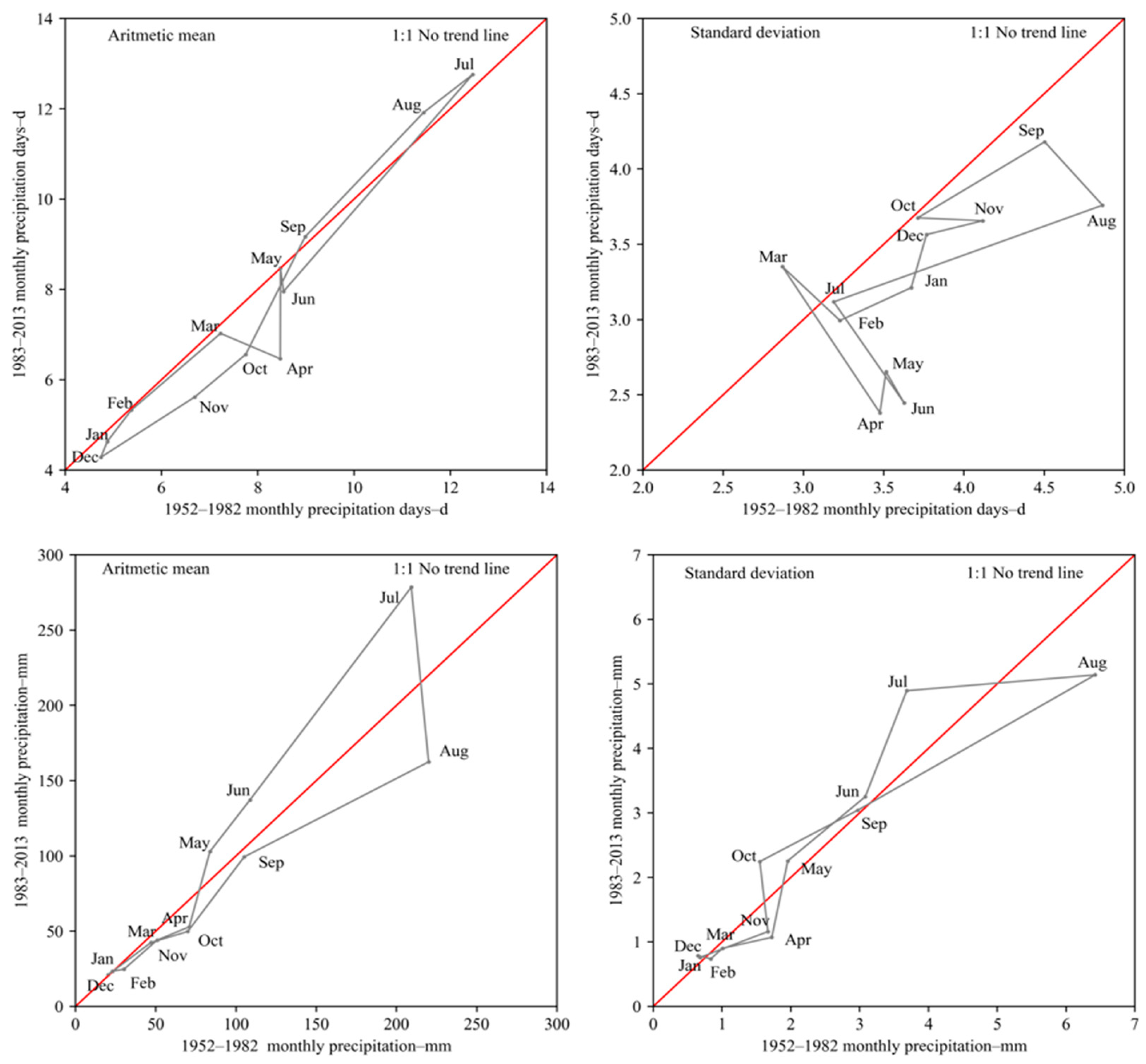
Seasonal precipitation at the Shimantan Reservoir was also analyzed during the period from 1956 to 2012. The annual changes in seasonal precipitation are shown in Figure 5. The results demonstrate that precipitation in summer (Figure 5b) captured the largest proportion among the four seasons, with an average value of 544 mm during the entire period. The average precipitation in spring (211 mm) (Figure 5a) basically equaled that in autumn (215 mm) (Figure 5c) from 1956–2021. 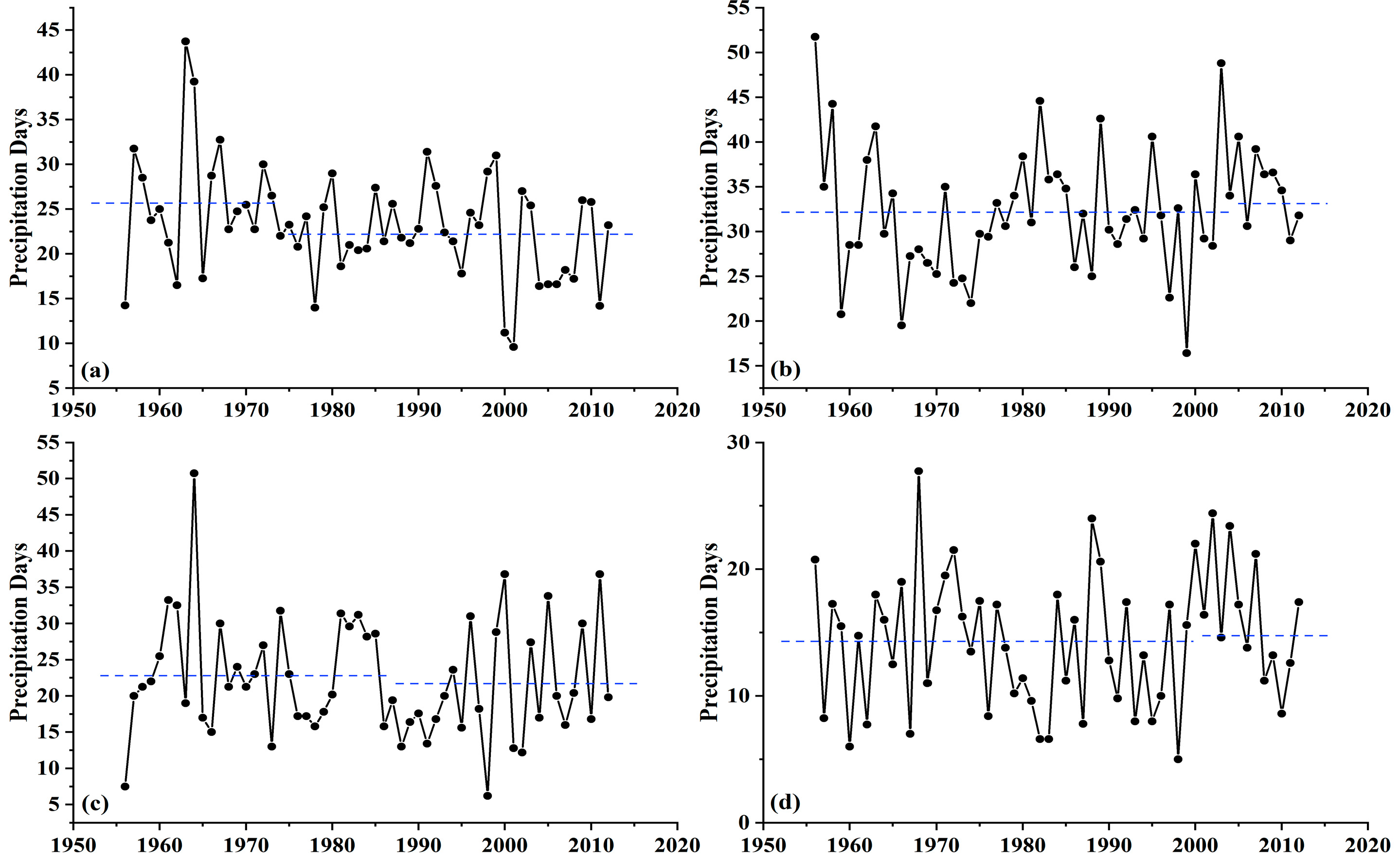Winter was the driest season, with an average precipitation of 72 mm (Figure 5d) from 1956–2012, which only accounted for 1/7 of the amount in summer. Precipitation days did not vary a lot among different seasons. The average precipitation days were 23.3 d, 32.3 d, 22.3 d, and 14.4 d in the spring (Figure 6a), summer (Figure 6b), autumn (Figure 6c), and winter (Figure 6d), respectively.

Some changing trends (increasing or decreasing) were observed for all four seasons, even though the trends were not statistically significant. For instance, based on the results of the moving t-test, we saw abruptly decreasing points of both spring precipitation and spring precipitation days (Figure 5a and Figure 6a). Summer precipitation demonstrated an abruptly increasing point in the year 1993, while summer precipitation days showed a small increasing point in the year 2004. Small decreasing points were observed for both autumn precipitation and autumn precipitation days, while winter changing trends were minimal.

In general, from 1956–2012, only summer precipitation increased at the Shimantan Reservoir, while the number of precipitation days increased slightly. This suggested that the average amount of a single precipitation day might increase, which is likely to aggravate the probability and magnitude of summer flooding. Furthermore, it is manifested in this study that both precipitation and precipitation days in spring and autumn, when it is usually lacking in precipitation, have decreased. This probably will result in a higher risk of droughts in these seasons. The increase in floods in summer and droughts in spring and autumn may have a negative impact on local agriculture. Meanwhile, as a large-scale water conservancy project focusing on flood control, industrial water supply, agricultural irrigation, and other comprehensive utilization functions, the Shimantan Reservoir should strengthen the reasonable regulation of water resources to prevent the occurrence of disastrous events downstream.

3.3. Variations in Summer Rainfall Events at the Shimantan Reservoir

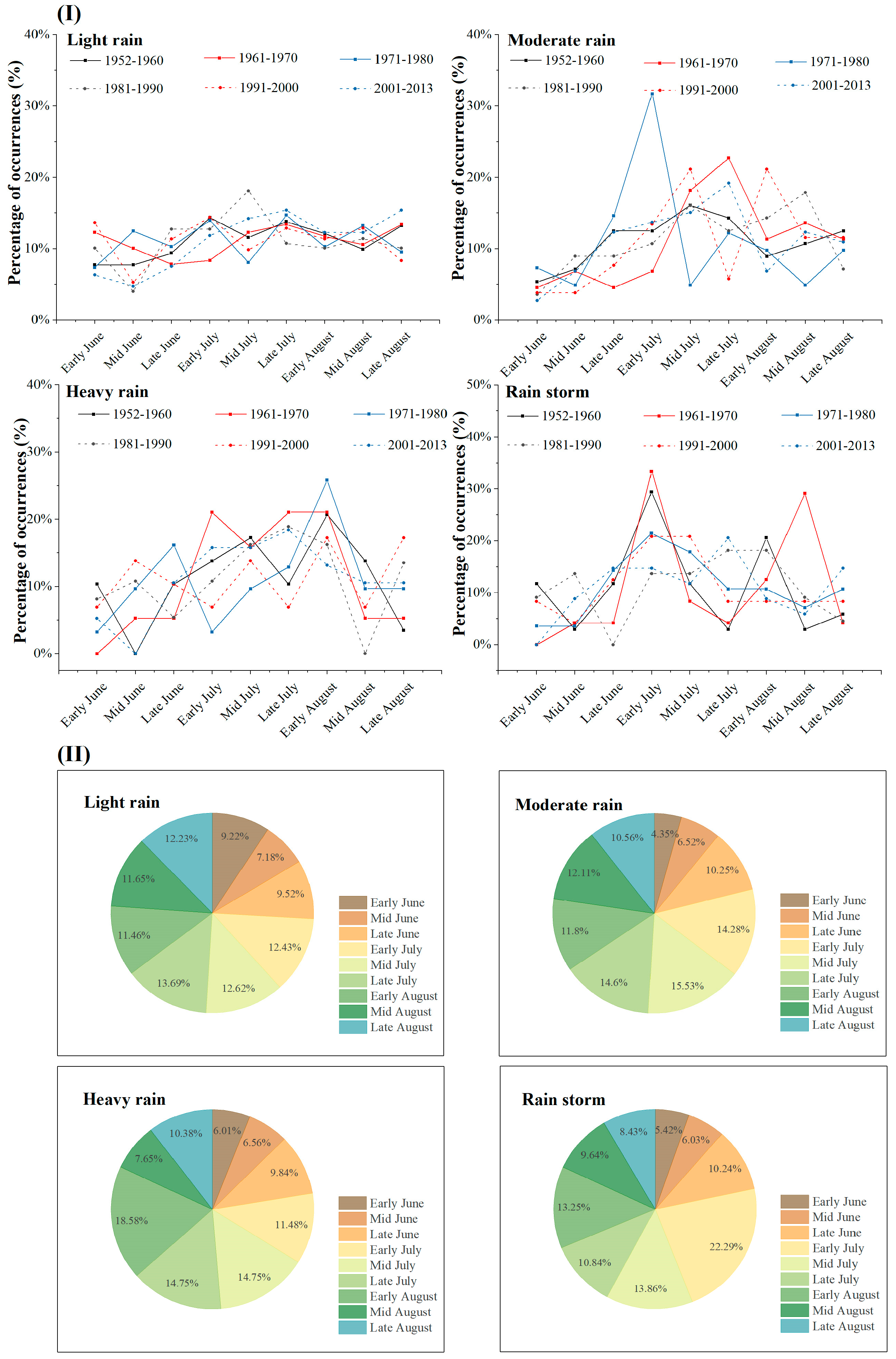
3.3.1. Occurrence Time of Rainfall Events of Different Levels

Rainfall events at the Shimantan Reservoir were categorized into four categories according to the total amounts of rainfall during events (i.e., <10 mm, 10–25 mm, 25–50 mm, and >50 mm) (Table 2). Figure 7 shows the changes in occurrence times of rainfall events for each level. In general, both light rain (<10 mm) and moderate rain (10–25 mm) events at the Shimantan Reservoir were concentrated in mid- and late July (Figure 7II). Heavy rain (25–50 mm) events mostly occurred in early August, with percentages ranging from 13.16% to 25.81% in different decades. Rainstorms exceeding 50 mm mainly occurred in early July. The percentage of these rainfall events in early July has declined from 29.41% in the 1950s to 14.71% in the 2000s. However, with the background of global climate change, the frequency of rainfall has increased in late July. The percentages of rainfall events in late July were 13.8%, 14.29%, 10.34%, and 2.94% for different levels (i.e., light rain, moderate rain, heavy rain, and rainstorms) from 1952–1960. For the period of 2001–2013, these percentages increased to 15.42%, 19.18%, 18.42%, and 20.59%, respectively. The percentage of light rain events did not show significant fluctuations within a year and remained relatively stable. On the other hand, the percentages of moderate rain events, heavy rain events, and rainstorm events in early August have decreased from 8.93%, 20.69%, and 20.59%, respectively, from 1952–1960, and to 6.85%, 13.16%, and 8.82%, respectively, from 2001–2013.

3.3.2. Occurrence Frequency of Summer Rainfall Events with Different Intensity

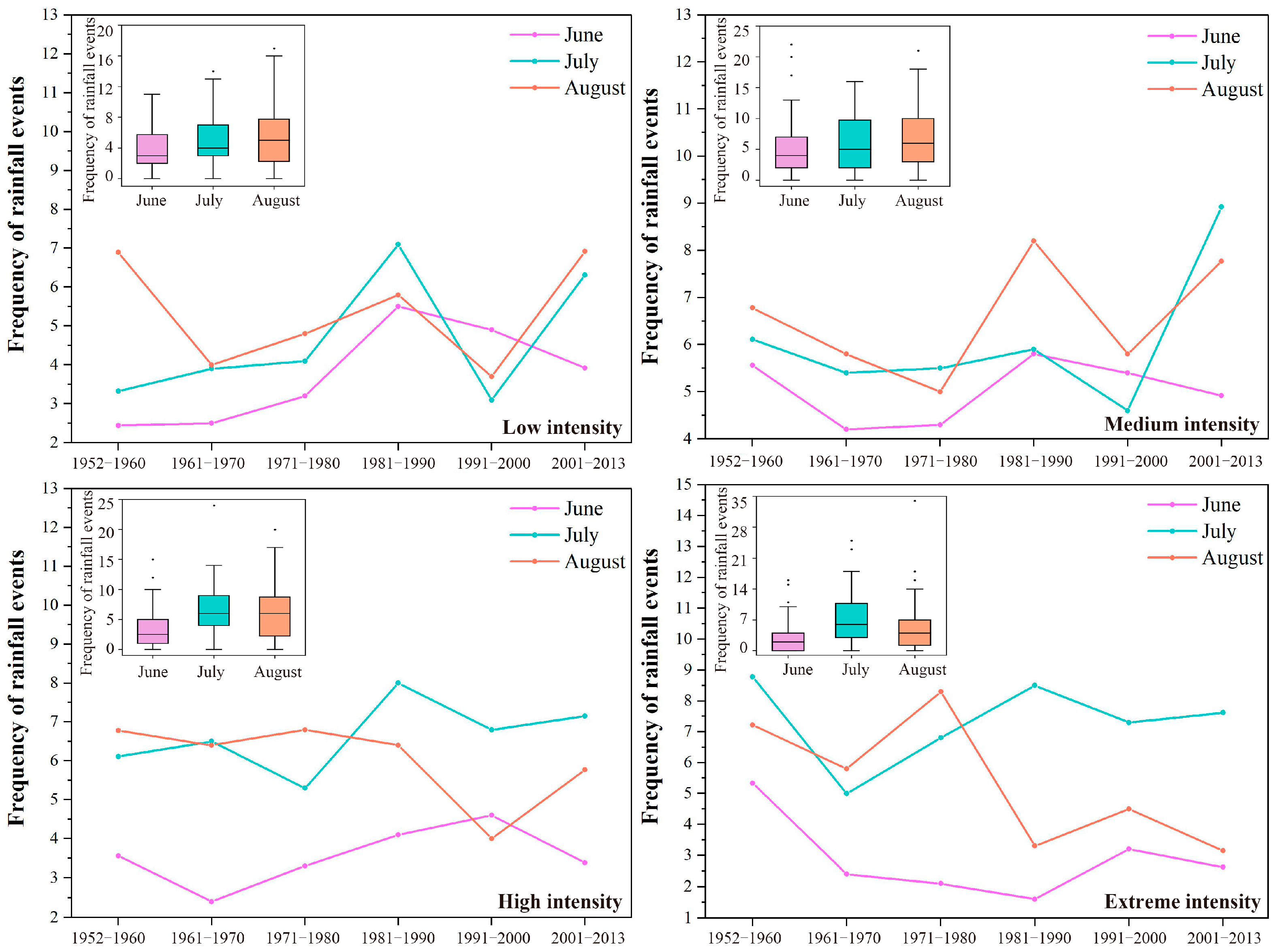
The variation in the frequency of rainfall events of different intensities at the Shimantan Reservoir is illustrated in Figure 8. During the study period, the frequency of rainfall events with low intensity (i.e., <2 mm/h) was obviously higher in August compared to June and July, except for the period of 1981–1990. The frequency of this type of rainfall event showed an increasing trend in June and July, except for the period of 1991–2000. The average number of occurrences of medium-intensity (2–4 mm/h) rainfall events during the study period was 6, with the maximum number of occurrences (i.e., 22) observed in June 2000. The frequency of this type of rainfall showed little variation among June, July, and August. Additionally, the frequency fluctuations in these three months were almost synchronous, with an alternating pattern of high to low.

The average frequency of high-intensity (4–8 mm/h) rainfall events was 3.56, 6.74, and 6.06 in June, July, and August, respectively. In June and August, high-intensity rainfall events occurred less frequently compared to medium and low-intensity events. Moreover, the frequency of rainfall events larger than 8 mm/h was smaller than that of any other type in June and August (Figure 8). In years with a high frequency of extreme rainfall events, heavy rains or floods were usually observed. For instance, the maximum frequency of 34 occurred in August 1975, which coincided with a historical torrential flood event that caused severe damage, according to historical data.

3.4. Variation Characteristics of Rainstorm Events at the Shimantan Reservoir

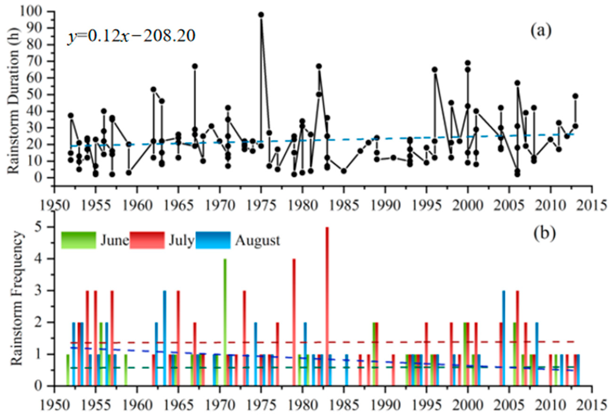
Figure 9 illustrates the duration (a) and frequency (b) variations in the rainstorm events at the Shimantan Reservoir. It can be seen that the duration of rainstorm events displayed obvious variation from 1952–2013, with the longest duration of 96 h in 1975 (Figure 9a). Generally, it showed an insignificantly upward trend with an increasing rate of 0.12 h/a.

According to statistics, a total of 137 rainstorms occurred at the Shimantan Reservoir from 1952 to 2013, and they were distributed in different summer months and years (Figure 9b). Consistent with the former analysis, the rainstorms in the study area mostly occurred in July, and the frequency was lowest in June. Among the months, there was an insignificantly upward trend both in June and July, while there was an obvious decline in August.

3.5. Influences of Atmospheric Circulations on Precipitation Changes at the Shimantan Reservoir

As stated above, the results of the present study suggested little change in annual precipitation during the study period of 1952–2013, but rainfall intensity and seasonal variation in precipitation at the Shimantan Reservoir were obvious, which likely aggravated both the frequency and magnitude of floods and droughts. Climate change is a key factor that disturbs hydrological processes. Climatic phenomena at different scales, i.e., global, regional, and micromorphological, have their respective impacts on regional hydrology.

In this paper, further investigation was undertaken to explore the reasons for precipitation variations at the Shimantan Reservoir in the past 61 years. Two indices, including the Arctic Oscillation (AO) and East Asian summer monsoon (EASM), one having global influences and the other mainly dominant in East Asia, were selected to seek out their relationships with precipitation eigenvalues.

3.5.1. Correlation between AO and Precipitation

Arctic Oscillation (AO) is a variation in atmospheric circulation at a planetary scale. The change in its intensity or location will have a significant impact on the global climate. The results of Pearson correlation analysis indicated that there were no significant linear relationships between the Arctic Oscillation (AO) and average monthly precipitation at the Shimantan Reservoir. The highest correlation coefficients were observed in May and October, both of which were 0.22 (p < 0.1) (

Table 5. Correlation between Arctic Oscillation (AO) and average monthly precipitation at the Shimantan Reservoir.

Month	January	February	March	April	May	June
Correlation	0.1	0.16	0.1	0.13	0.22 *	0.13
Month	July	August	September	October	November	December
Correlation	0.06	0.03	−0.09	0.22 *	−0.03	0.03

Notes: * represents a correlation coefficient that has passed the significance level of 0.1.

).

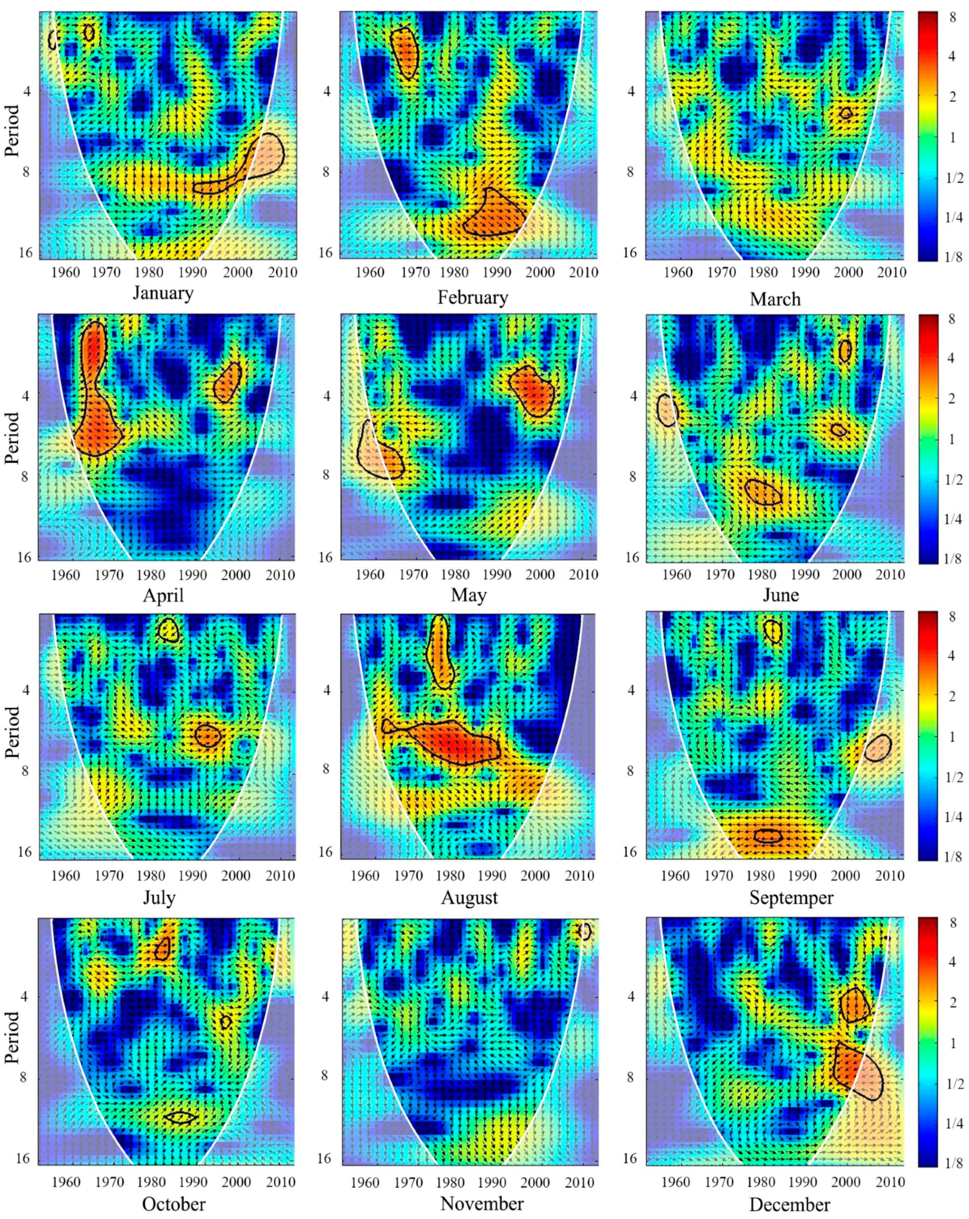
Cross-wavelet power spectra and coherent spectra were also applied to make a comprehensive description of the relationship between AO and monthly precipitation at the Shimantan Reservoir, and the results are shown in Figure 10. In Figure 10, the thick black lines, represented by circles, signify the areas that have passed the significance test against red noise at a 0.05 level, while the white lines represent the boundaries of the wavelet influence cones. The phase differences between the two series are indicated by arrows in the figures. Arrows pointing to the right suggest that AO and monthly precipitation are in phase, and there is basically a positive correlation between them. Meanwhile, arrows pointing to the left indicate that the two series are out of phase or they have a negative cyclical effect on each other. Arrows pointing down indicate that the change in AO is ahead of the change in precipitation by π/2 phases, with a corresponding time of 3 months, while arrows pointing up indicate that the change in the AO is posterior to the change in precipitation by π/2 phases (i.e., 3 months).

It is interesting to see that the directions of arrows at different frequency bands over the study period (1952–2013) were different (Figure 10), indicating different effects of AO and monthly precipitation on each other. Generally, a positive correlation was found between AO and precipitation in the winter and spring months, and the phase differences varied in the range from π/4 to 3π/4, while the relationship in summer and autumn was not remarkable and varied undirectedly during the study period. For example, AO and January precipitation were in phase and exhibited a cyclical effect of 6~8 years. AO and February precipitation were in phase for a scale of 3–4 years from 1968–1972 and a scale of 10–12 years from 1980–1995. For the period from 1960–1970, in the 1~7-years scale, we found evidence of cyclical effects (in phase) of AO and precipitation in April, with high power. In June, July, and September, the two indices only experienced irregular fluctuations of low energy. The phase difference was insignificant and sometimes the relationship was totally inverse, which should be discussed in further research.

It can be concluded that AO had an important impact on precipitation in winter and spring at the Shimantan Reservoir. The significant oscillations between AO and precipitation indicated varying phase differences at different times and frequencies, which imposed direct or indirect influences on the change in precipitation in the region.

3.5.2. Correlation between EASM and Frequencies of Different Rainfalls with Intensities in Summer

The Shimantan Reservoir is located in Henan Province, at the junction of the East Asian monsoon region and the East Asian summer monsoon region. Hydrology in such areas is characterized by the East Asian summer monsoon (EASM) pattern to varying degrees, in which the beginning of the summer monsoon brings the rainy season, and in contrast, its retreat marks the end. Therefore, it is of great significance to conduct regional studies of changes in summer monsoons for understanding the dry–wet transition of rainy seasons, and to perform analysis of abnormal hydrological variables.

Identified by Pearson correlation analysis, an entirely inverse correlation was demonstrated between the EASM and the frequencies of different rainfall intensities in summer (

Table 6. Correlation between the East Asian summer monsoon (EASM) and occurrences of rainfalls with different intensities.

Rainfall Intensity	EASM
	June	July	August
Low intensity (<2 mm/h)	−0.20	−0.054	−0.17
Medium intensity (2–4 mm/h)	−0.21	−0.12	−0.25 **
High intensity (4–8 mm/h)	−0.40 ***	−0.14	−0.20
Extreme intensity (>8 mm/h)	−0.23 *	−0.012	−0.10

Notes: EASM is short for East Asian summer monsoon. An asterisk (*), double asterisks (**), and triple asterisks (***) represent correlation coefficients that have passed the significance levels of 0.1, 0.05, and 0.01, respectively.

). It can be understood in a more practical way; a year with a strong monsoon usually has fewer summer rainfall events, no matter which kind. From the perspective of a correlation coefficient, there is no clear linear correlation between the East Asian summer monsoon (EASM) and the occurrence of rainfall with different intensities in July. However, in August, medium-intensity rainfall showed a relatively large correlation coefficient with the EASM (p < 0.05). On the other hand, rainfall events of high and extreme intensities exhibited larger correlation coefficients with the EASM in June, with coefficients of −0.40 (p < 0.01) and −0.23 (p < 0.1), respectively.

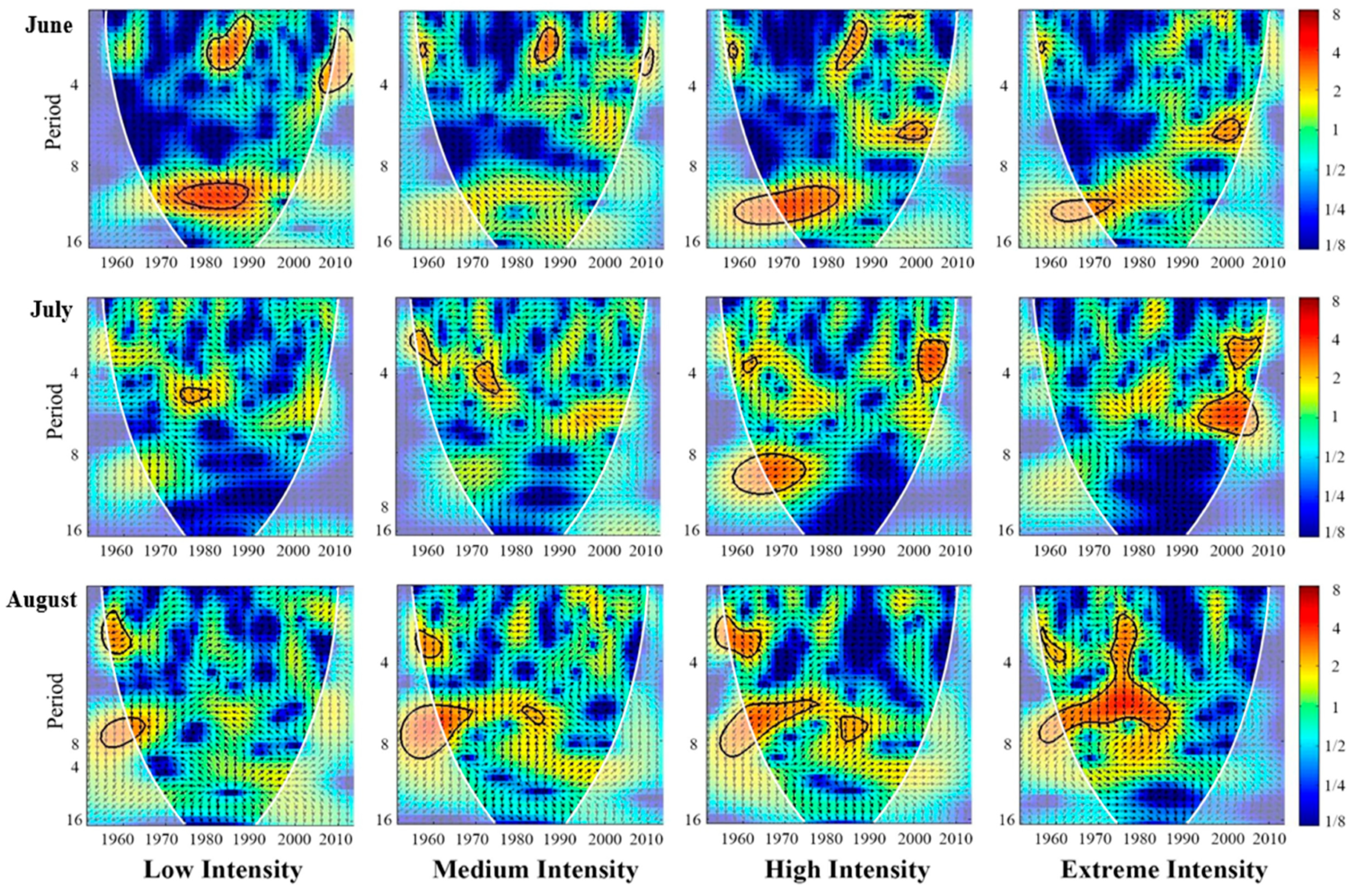
The cross-wavelet power spectra and coherent spectra of the EASM and the frequency of summer rainfall intensity at the Shimantan Reservoir are shown in Figure 11. A negative correlation can be found between the EASM and the frequency of summer rainfall intensity at the Shimantan Reservoir during the study period, and an oscillation with a large span of 2–12 years was exhibited (Figure 11). The correlation varied among different months and levels of rainfall intensity. The oscillation period changed irregularly in June and July, while in August, the correlation between rain intensity frequency and the EASM increased with the increase in rain intensity frequency. When it rained with medium or high intensity, the time–frequency variation was clearly consistent among these three months. However, the consistency was destroyed when it came to precipitation of low or extreme intensity. Under a comprehensive analysis of these findings using the geographical location of the study area and the characteristics of the EASM, it is possible to speculate that the differences in the correlations between the two indices may be related to the transport intensity of the southerly monsoon and different locations of water vapor convergence.

Changes in both the Arctic Oscillation and the East Asian summer monsoon affected precipitation patterns at the Shimantan Reservoir, and the influence of the EASM on summer precipitation is more significant than that of AO.

Similar conclusions can be derived from previous research [47,48,49,50,51]. During winter, the abnormal atmospheric circulation in East Asia, caused by the inter-decadal anomaly of the AO, leads to changes in the intensity of the East Asian monsoon. This affects the frequency of cold air moving southward and the intensity of the Mongolian high pressure, ultimately influencing the winter precipitation changes in the area where the Shimantan Reservoir is located [47]. In summer, AO impacts the intensity of the EASM, resulting in variations in the onset and retreat times, motion speeds, and stagnation times of the monsoon rain belt. This ultimately leads to abnormal summer precipitation in the area where the Shimantan Reservoir is situated [51].

It is important to note that previous studies on AO, the EASM, and climate change have primarily focused on large-scale regions [52,53,54]. However, this study provides evidence that the research conclusions from these large-scale studies are also applicable to small watersheds. Therefore, decision makers and stakeholders in small watersheds can refer to the conclusions of large-scale research when making watershed-related decisions and assessing change risks. This will provide convenience and advantages for the development and implementation of adaptive strategies under climate change conditions.

3.6. Implications for Regional Rainfall Climatology and Hydrologic Designs

The changes in precipitation characteristics at the Shimantan Reservoir are a specific response to the global climate change observed in recent decades [55]. Despite a slight increase in annual precipitation, there is a noticeable rise in the proportion of summer rainfall as a part of the total annual precipitation, accompanied by a decrease in the number of precipitation days. This indicates a shift in the intra-annual pattern of regional rainfall. The concentration of rainfall in fewer summer days increases the likelihood of more intense summer rainfall, which aligns with the scientific understanding that extreme precipitation tends to intensify more rapidly than average precipitation in a warming climate [56,57]. However, this increase in extreme summer rainfall can have unprecedented impacts on various aspects such as public health, society, economy, and ecology. For example, excessive and intense rainfall can lead to significant economic losses due to crop failures on the large-scale North China Plain [58]. Considering the crucial role of this region in China’s crop production [59], the negative impact can extend across the entire country. Additionally, the possibility of drought is also heightened outside of the summer season, posing a significant threat to domestic, agricultural, and industrial water needs in this densely populated and climate-sensitive region [60,61]. To mitigate the future economic losses caused by climate change, it would be beneficial for local farmers to adapt their farming practices and crop choices. Furthermore, engineering practices should be guided by scientific principles to strike a balance between safety and necessity. Implementation of non-structural measures, such as providing practical guidance to the public, can help reduce the extent of these losses to an acceptable degree.

During the study period, the rainfall climatology showed an increase in extreme and catastrophic floods due to a thicker upper tail [62,63]. In recent years, North China has experienced catastrophic extreme rainfall and flooding, such as the ‘21.7′ extreme rainfall in Henan Province and the ‘23.7′ extreme rainfall in Beijing and the surrounding regions. These events have resulted in numerous casualties and significant consequences, particularly in highly developed metropolises like Zhengzhou and Beijing. The more severe and frequent floods pose new challenges to the design standards of contemporary flood control infrastructures. Additionally, the conventional methods of estimating precipitation for hydrological designs, known as design storms, have proven to be ineffective in maintaining their function under a changing climate [64,65,66]. It is crucial to review the applicability of these designs from a scientific perspective and update them to a more reliable level if economically feasible.

Our study observes a remarkable precipitation response at shorter temporal scales, specifically at the seasonal and daily scales. In fact, rainfall extremes increase even more rapidly at the sub-daily and sub-hourly scales [67,68], indicating a scale-dependent rainfall response to climate change [69]. Further research is needed to investigate the mechanisms behind this response, including atmospheric circulations, land–atmosphere interaction, and anthropogenic climate change. Additionally, our study found that both annual and summer precipitation showed an upward trend at the Shimantan Reservoir. But the changing rate of summer precipitation was greater than that of annual precipitation. As for precipitation days, annual precipitation days displayed an insignificant (α = 0.05) decreasing trend. This indicates that the intensity of precipitation has increased, especially in the summer, which means there is a higher possibility of extreme precipitation events at the Shimantan Reservoir. It is expected that the spatial patterns and temporal variations in precipitation will substantially change with global warming. While our study does not focus on the response of precipitation to the warming climate, future research should explore precipitation patterns under different climate scenarios. A precise understanding of rainfall climatology, improved simulation of fine-scale extreme rainfall events, and accurate estimation of design storms are essential to comprehensively grasp regional rainfall patterns. This knowledge will enable the development of reasonable measures and schedules for flood control and sustainable development in the target region.

4. Conclusions

Intensified precipitation due to atmospheric warming has been observed globally, emphasizing the need for a comprehensive investigation into the spatial and temporal patterns as well as the mechanisms of precipitation. In this study, we analyzed the daily precipitation data from six stations at the Shimantan Reservoir spanning from 1952 to 2013. Our aim was to examine the characteristics of precipitation at different time scales. We employed statistical analysis to detect trends and change points in the total precipitation amount, frequency, and duration. Furthermore, we explored the influence of atmospheric circulations on precipitation using cross-wavelet analysis. Our results demonstrate that the characteristics of precipitation at the Shimantan Reservoir have undergone varying degrees of change, and in different directions, during the study period of 1952–2013. The key findings of our study can be summarized as follows:

The precipitation amount and precipitation days at the Shimantan Reservoir contributed significantly to the effects in July and August. The reservoir experienced a positive trend in summer precipitation, while the trend for annual precipitation days was reversed. These findings suggest a potential increase in extreme precipitation events. The IPTA method can provide additional insights to complement the Mann–Kendall test. According to the IPTA method, there was a noticeable transition trend from an increase to a decrease in precipitation from July to August, and a transition from a decrease to an increase in precipitation days from June to July.

The distribution of precipitation events with different levels varied significantly throughout the year. Extreme precipitation events with amounts exceeding 50 mm mainly occurred in early July. It is important to pay close attention to preventive measures for rainstorms and flood events in July, especially in early July.

The intensity of summer rainfall events is always extremely high in July. The duration of summer rainstorms fluctuates greatly and shows a trend of shortening. However, the occurrence of rainstorms has not changed much over the years, which can be an important reference for predicting heavy rains.

The Shimantan Reservoir is influenced by the Arctic Oscillation (AO) and the East Asian summer monsoon (EASM). Changes in the duration and frequency of AO and the EASM will affect the precipitation in the study area to varying degrees.

Overall, our study provides a refined description of precipitation patterns and mechanisms under climate change conditions, benefiting regional flood control and sustainable development.