Article

Coil System Design for Multi-Frequency Resistivity Logging Tool Based on Numerical Simulation

1
School of Geosciences and Technology, Southwest Petroleum University, Chengdu 610500, China
2
College of Geophysics, China University of Petroleum-Beijing, Beijing 102249, China
3
Western Australian School of Mines, Energy and Chemical Engineering, Curtin University, Perth 6845, Australia
*
Author to whom correspondence should be addressed.
Water 2023, 15(24), 4213; https://doi.org/10.3390/w15244213
Submission received: 24 October 2023 / Revised: 1 December 2023 / Accepted: 4 December 2023 / Published: 6 December 2023
(This article belongs to the Special Issue Groundwater Exploration and Hydrogeophysical Research)

Abstract

:
A coil-type resistivity logging tool has been proposed for multi-frequency operation (250 kHz to 8 MHz) based on electromagnetic wave propagation. Different frequencies are matched with specific transmission coils, while the same two reception coils are used to achieve a consistent depth of investigation (DOI). By analyzing the electromagnetic attenuation and phase difference of induced signals at different frequencies, the complex resistivity can be jointly inverted. The coil systems were designed with four DOI options (0.3 m, 0.5 m, 1 m, and 1.5 m) and six measurement frequencies (250 kHz, 500 kHz, 1 MHz, 2 MHz, 4 MHz, and 8 MHz). Their detection performance was evaluated using the finite element method on the COMSOL platform. For higher frequencies or a deeper DOI, a coil system with a larger source-receiver distance was selected. These designed coil systems can provide qualitative identification of formations with thicknesses greater than 0.05 m and quantitative identification of formations with thicknesses greater than 1.5 m. In the single-transmission, dual-reception coil system, response signals are distorted at the formation boundary, and this distortion increases with the source-receiver distance. Adding a secondary transmission coil can reduce the distortion of response signals at the formation interface without increasing the overall length of the coil system. This research enriches the theoretical framework of complex resistivity spectrum (CRS) logging and contributes to the commercial development of CRS logging tools.

1. Introduction

Resistivity logging data are crucial for evaluating formation water saturation [1]. However, conventional resistivity logging tools encounter challenges when assessing the saturation of low-resistivity formations, as the difference in resistivity between oil and water reservoirs is small. Rock’s complex resistivity provides both resistivity and dielectric constant information about formations [2], which changes with variations in measurement frequency, displaying a pattern known as the complex resistivity spectrum (CRS). Experiments have shown that reservoir parameters such as porosity, permeability, water saturation, and water salinity influence the CRS characteristics of the formation [3,4,5,6,7,8]. Consequently, numerous evaluation methods for reservoir parameters based on CRS have emerged [9,10,11], showing promising potential in the exploration of oil and gas resources [12].
The development of the CRS logging tool lags behind the petrophysics experiment study of the dispersion mechanism of CRS. Currently, there are commercial multi-frequency resistivity logging tools [13,14,15,16,17], which aim to acquire resistivity information at different Depths of Investigation (DOI) by increasing the number of measurement frequencies. However, due to the invasion of mud, the formation medium near the wellbore exhibits significant heterogeneity with increasing radial depth, rendering the real spectrum measurement unattainable for these tools. While the dielectric scanner by Schlumberger measures the conductivity and permittivity of formations at four frequencies from 20 MHz to 1 GHz [18,19,20,21,22], other logging tools utilizing a complex resistivity spectrum have not emerged. Consequently, many research results have not been effectively utilized in geophysical logging.
The Electric Logging Laboratory of China University of Petroleum-Beijing has developed a prototype electrode-type CRS logging tool based on the dual-lateral logging tool and established an indoor experimental system [23] to obtain the complete CRS of formations in the frequency range of 1–500 kHz. However, this frequency band may not fully meet the logging requirements of complex geological profiles such as low porosity and low permeability reservoirs. For certain low-porosity and low-permeability rock samples, the impedance dispersion features correspond to frequency ranges exceeding 500 kHz (see Figure 1) [11]. Therefore, it is crucial to enhance the CRS logging theory and design a new type of CRS logging tool with a higher measurement frequency band to achieve a more precise assessment of a reservoir’s porosity structure, water saturation, and permeability parameters. The electrode-type focusing measurement method is unsuitable for high-frequency measurements due to the difficulty of radiating excitation signal energy into the formation [24]. Coil-type logging tools are more suitable for measuring the high-frequency resistivity of formations [25]. This paper conducted a numerical simulation study to design a coil-type CRS logging tool capable of measuring CRS in the frequency band of 250 kHz–8 MHz and investigated its detection characteristics.

2. Principle and Method

2.1. Measuring Principle

The measurement unit of the tool for each individual frequency is designed as a single-transmission and dual-reception coil system, as shown in Figure 2. The system utilizes electromagnetic wave propagation to measure the properties of the formation. In this system, an alternating current excitation (ACE) with a fixed frequency is applied to the transmission coil T. Two reception coils, R1 and R2, are used to detect the electromagnetic signals induced by the transmission coil.
The amplitude and phase of the voltage signals induced by R1 and R2 are collected, and the electromagnetic attenuation (EATT) and phase difference (Δφ) can be calculated using the following formulas [26]:
E A T T = 20 lg V 2 V 1
Δ φ = φ 1 φ 2
where, V 1 and φ 1 are the amplitude and phase of the induced voltage on the reception coil R1, and V 2 and φ 2 are the amplitude and phase of the induced voltage on the reception coil R2. EATT is primarily influenced by the conductivity of the medium along the electromagnetic wave propagation path, while the phase difference signal is mainly affected by the dielectric constant of the medium.
Chu et al. [27] provided the analytical expressions for EATT and Δφ of the induced signals in the single-transmission and dual-reception coil system.
E A T T = 20 lg V 2 V 1 = 10 lg α L 2 2 + ( 1 + β L 2 ) 2 α L 1 2 + ( 1 + β L 1 ) 2 + 60 lg L 1 L 2 + 8.686 β ( L 1 L 2 )
Δ φ = φ 1 φ 2 = α ( L 2 L 1 ) + arctan 1 + β L 2 α L 2 arctan 1 + β L 1 α L 1
α = ω 1 2 μ ε 2 + σ 2 ω 2 + ε β = ω 1 2 μ ε 2 + σ 2 ω 2 ε
where, ω is the angular frequency, and ε , σ and μ are the dielectric constant, conductivity, and magnetic permeability of the medium. L1 and L2 are the distance between the transmission coil with the two reception coils, where L2 > L1.
Equations (3)–(5) demonstrate that both EATT and Δφ depend on the dielectric constant and conductivity. In conventional tools with high measurement frequency, the dielectric constant is typically considered constant due to its small value and weak dispersion. This allows for the independent inversion of resistivity using either the EATT or Δφ signal, resulting in two types of resistivity curves: electromagnetic attenuation resistivity and phase difference resistivity.
However, in the measurement frequency range of a coil-type multi-frequency resistivity logging tool, the dielectric constant cannot be assumed as a fixed value since it is part of the complex resistivity. Therefore, a combination of EATT and Δφ is required to invert both the dielectric constant and conductivity of the formation. This enables the calculation of the complex resistivity [28].
ρ * ( ω ) = ρ ( ω ) + j ρ ( ω ) = σ a σ a 2 + ω ε a 2 j ω ε a σ a 2 + ω ε a 2
where, j is the imaginary unit, ρ * ( ω ) is the complex resistivity, and ρ ( ω ) and ρ ( ω ) are its real and imaginary parts, respectively. ε a and σ a are the inverted dielectric constant and conductivity.
The coil-type multi-frequency resistivity logging tool is designed to measure the complex resistivity at six discrete frequencies (250 kHz, 500 kHz, 1 MHz, 2 MHz, 4 MHz, and 8 MHz) with the same depth of investigation (DOI). The resistivity spectrum can be obtained by using impedance dispersion models [8,17] based on measured data from all six frequencies [23].
However, due to the skin effect, the single-transmission and dual-reception coil system (shown in Figure 2) has varying DOI values at different frequencies. As a result, multiple transmission coils with different source-receiver distances are necessary to maintain the same DOI when measuring at different frequencies. It is important to investigate how source-receiver distances and measurement frequency affect the detection performance of the coil system to optimize its design structure.

2.2. Simulation Method

The COMSOL platform was utilized for finite element analysis to optimize the structure of the coil systems and assess their detection performance. This study primarily focuses on the detection performance and structural optimization of the coil-type multi-frequency resistivity logging tool. The coil system is assumed to exhibit axisymmetric characteristics for isotropic formations, and for simplicity, the anisotropy of the formation is disregarded. Consequently, a 2D axisymmetric model was employed for simulation, significantly reducing the computational workload.
To compare simulation results with analytical solutions, a single-transmission and dual-reception coil system with a single turn was placed in a homogeneous model with varying formation conductivities, and the measurement frequency was set to 8 MHz. The analytical solutions for EATT and Δφ are provided in Equations (3)–(6). As depicted in Figure 3, the simulation results closely align with the analytical solutions, demonstrating a relative error of less than 2%. This indicates the viability of the simulation method employed in this study.

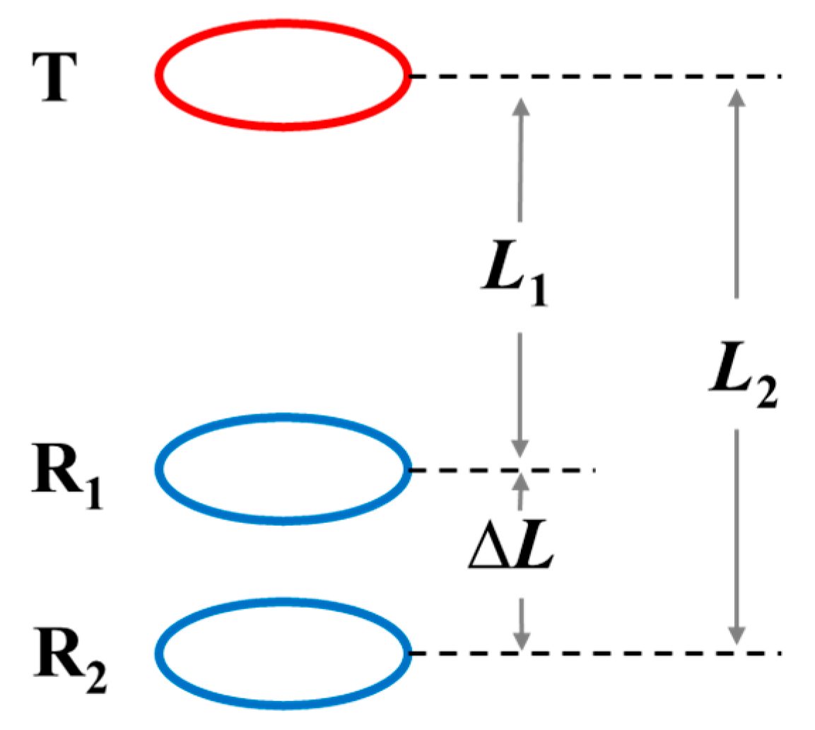
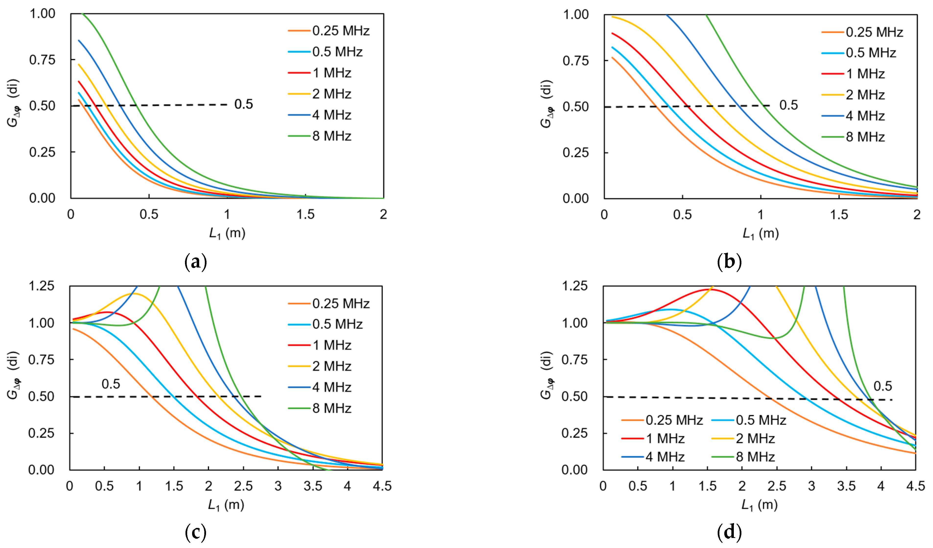
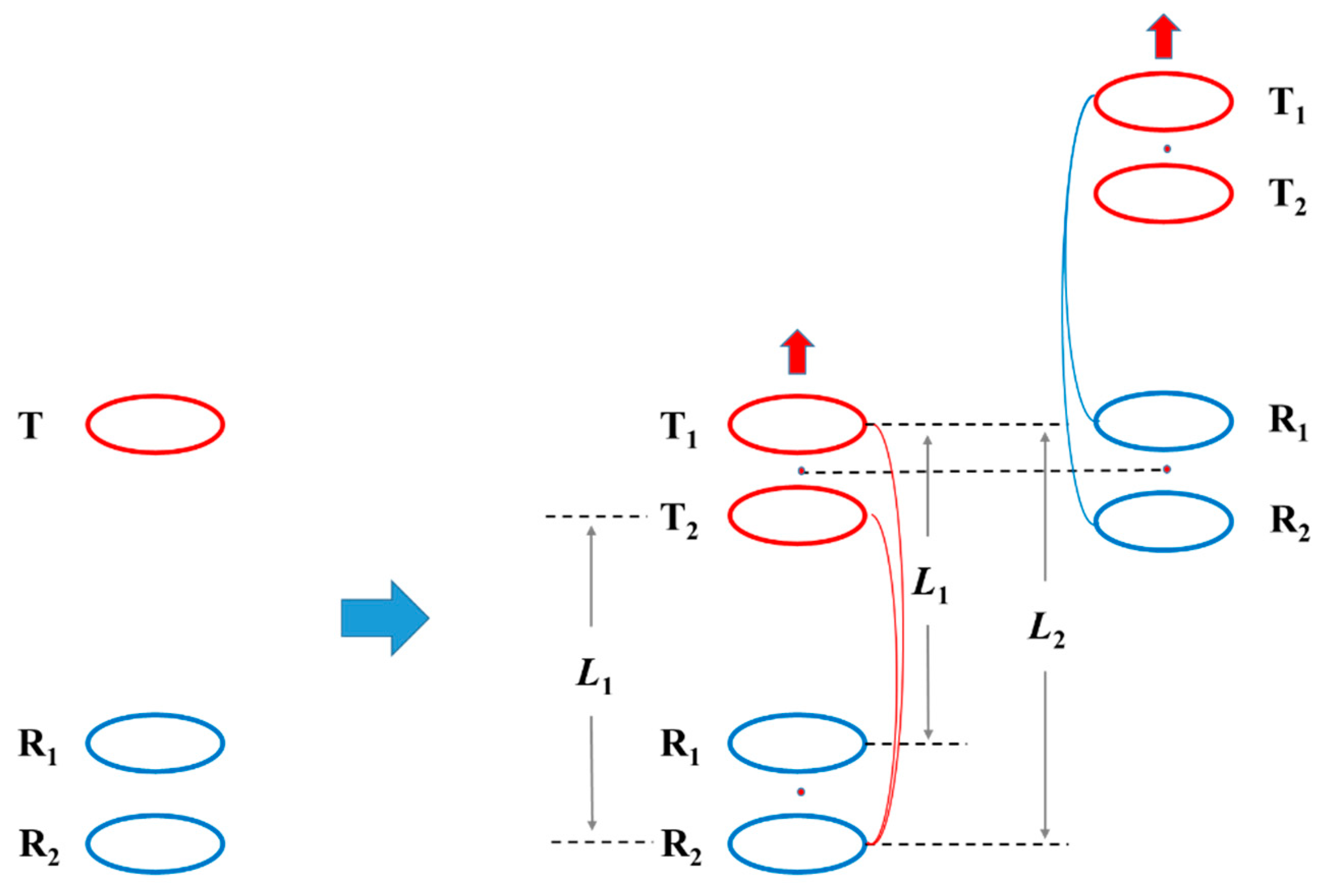
2.3. Determine the Source-Receiver Distance

In numerical simulations, the depth of investigation (DOI) for the resistivity logging tool is typically evaluated using pseudo-geometric factor theory [29]. The medium model comprises only the invasion zone and the intact zone when the effects of the borehole are ignored. There should be a correlation between the apparent conductivity and the conductivity of each component, which can be expressed as follows:
σ a = σ i 0 d i g ( r ) d r + σ t d i g ( r ) d r
where, σ a is the apparent conductivity, and σ i and σ t are the conductivity of the invasion zone and the intact zone, respectively. di is the depth of the invasion, and g(r) is the radial differential geometric factor.
According to the definition, the radial integral geometric factor is:
G ( r ) = 0 r g ( r ) d r
The radial integral geometric factor represents the proportionate contribution of an infinitely tall cylinder with a radius of r to the measurement result, which approaches 1 as r tends towards infinity. Thus, Equation (7) can be rewritten as follows:
σ a = σ i G ( d i ) + σ t ( 1 G ( d i ) )
Then,
G ( d i ) = σ a σ t σ i σ t
where G ( d i ) is the pseudo integral geometry factor, and the corresponding invasion depth when G ( d i ) = 0.5 is defined as the DOI of the tool.
The measurement signal of the coil-type multi-frequency resistivity logging tool is EATT and Δφ, which are induced signals from the two reception coils. The information reflected by Δφ is shallower than that of EATT. Hence, a new pseudo integral geometric factor is defined using the Δφ signal to investigate the depth of investigation (DOI) of the coil system in this study:
G Δ φ ( d i ) = Δ φ a Δ φ t Δ φ i Δ φ t
where Δ φ a is the apparent phase difference, and Δ φ i and Δ φ t are the phase difference when the detection model is pure invasion zone and intact zone, respectively.
A three-layer medium model, as shown in Figure 4, is established to incorporate the effect of drilling mud. This approach aims to obtain a DOI that is as accurate as possible in actual logging environments. Δ φ a , Δ φ i , and Δ φ t all contain the response signal of drilling mud.
To evaluate the DOI of a resistivity logging tool, it is typically necessary to vary the radius of the invasion zone in the model and observe how the pseudo integral geometric factor changes. However, since the purpose of this study is to design a coil system with a specific DOI, we have set the radius of the invasion zone as our fixed target DOI, with a ΔL of 0.2 m. The key parameters of the model are listed in Table 1.
We conducted simulations by varying L1 to investigate the impact of changing it on the pseudo integral geometric factor. Through these simulations, we could determine the change in both the pseudo integral geometric factor and Δφ with respect to L1. Using Equation (11), we calculated the change in the pseudo integral geometric factor with respect to L1. Finally, we selected an appropriate value of L1 as the design outcome when the pseudo integral geometric factor was equivalent to the target value. This process significantly expedites the optimization of the coil system.

3. Result and Discussion

3.1. Structure of Coil Systems

Figure 5 illustrates the change in G Δ φ ( d i ) with respect to L1 for the target DOI of 0.3 m, 0.5 m, 1 m, and 1.5 m. When L1 is fixed, higher measurement frequencies correspond to larger values of G Δ φ ( d i ) . Therefore, to ensure that different frequencies correspond to the same DOI, a high measurement frequency should be paired with a transmission coil that has a larger L1. By examining the L1 value associated with each curve in Figure 5 when G Δ φ ( d i ) = 0.5 , Table 2 provides the values of L1 and L2 for single-transmission dual-reception coil systems that meet the requirements for each target DOI and measurement frequency. Based on the information from Table 2, six-transmission dual-reception coil systems can be designed to conduct measurements at six frequencies with the same DOI, as presented in Table 3.
By utilizing the six-transmission dual-reception coil system structure described in Table 3, it is possible to achieve multi-frequency complex resistivity measurements with the same depth of investigation (DOI) by matching different measuring frequencies with their corresponding transmission coils. If more transmission coils are integrated into a single tool, such as a 12- or 18-transmission dual-reception coil system, it becomes feasible to conduct measurements with multiple frequencies and multiple DOIs using a single tool. This expanded capability allows for more comprehensive data acquisition and analysis, providing a deeper understanding of the subsurface formation properties.

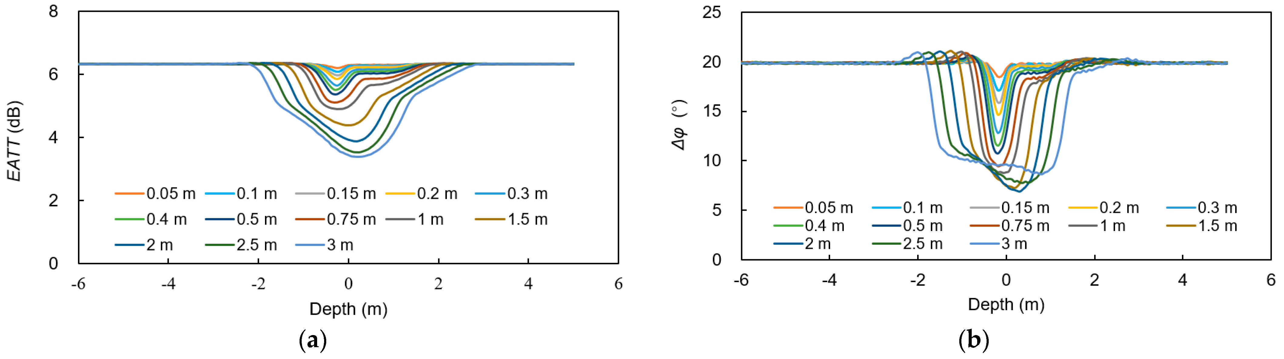
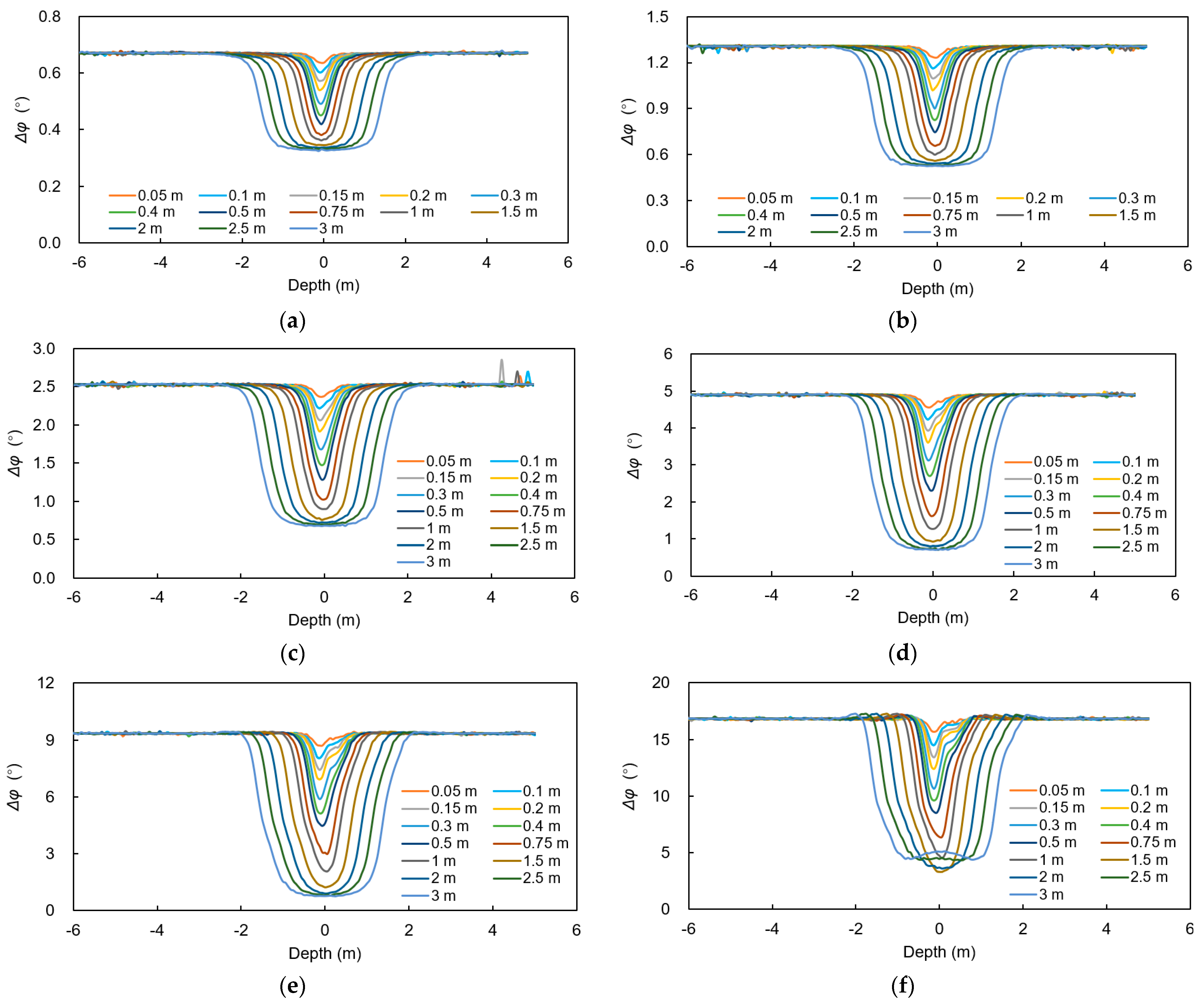
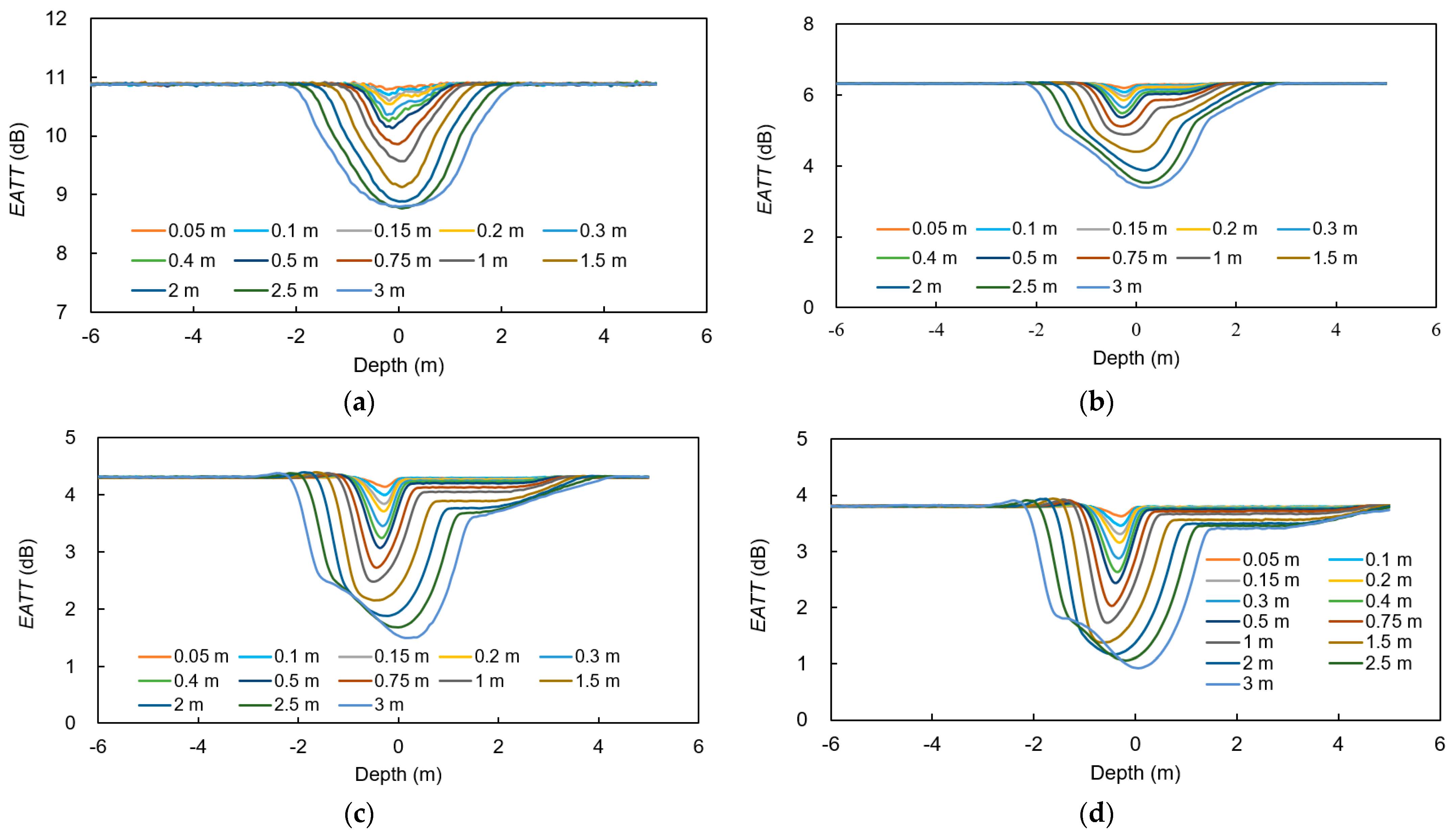
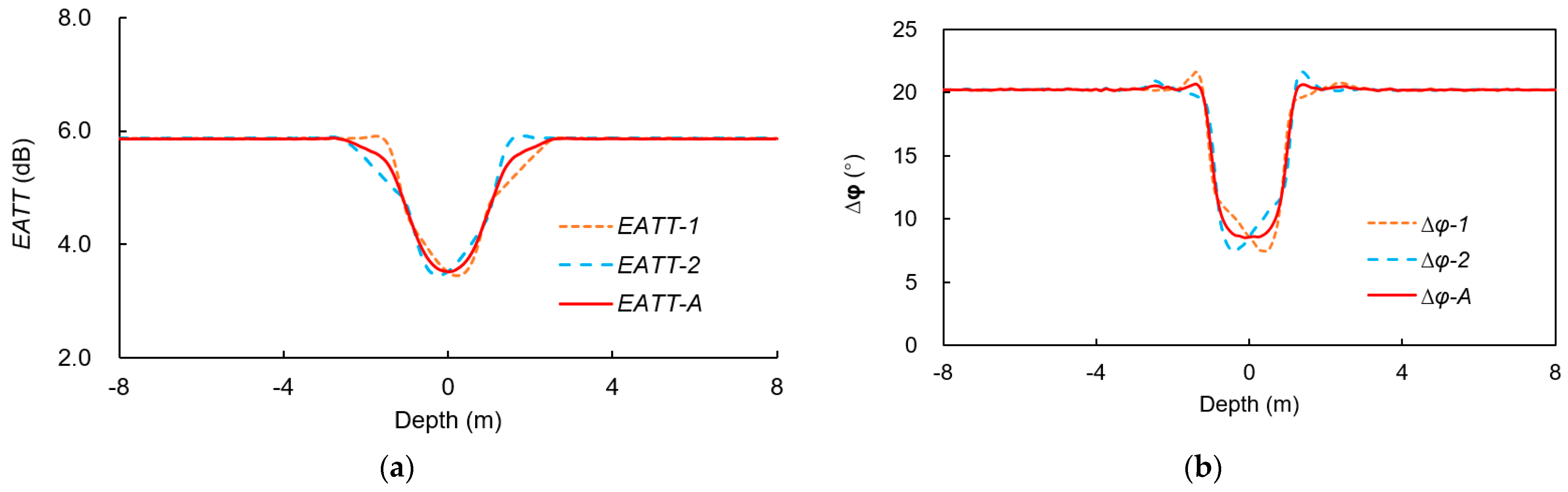
3.2. Vertical Resolution

The investigation of the vertical resolution of the coil system structures involved the design of a three-layer formation model with a wellbore and varying thickness of the target layer, as illustrated in Figure 6. The selected thicknesses of the target layer (H) were as follows: 0.05 m, 0.1 m, 0.15 m, 0.2 m, 0.3 m, 0.4 m, 0.5 m, 0.75 m, 1 m, 1.5 m, 2 m, 2.5 m, and 3 m. Additional parameters of the model are presented in Table 4.
By conducting simulations based on this model, the vertical resolution of the coil system structures can be thoroughly evaluated across varying thicknesses of the target layer. This analysis will provide insights into the system’s ability to distinguish and characterize the properties of different layers within the subsurface formation. Such assessments are crucial for optimizing the performance and applicability of the coil system in practical logging operations.
In Figure 7, the response curves of both EATT and Δφ are depicted for the coil systems with a DOI of 0.5 m, using a measurement frequency of 8 MHz. These curves represent the behavior of the coil system when different thicknesses of the target layer are present. It can be observed that both EATT and Δφ values in response to the target layer are smaller compared to the surrounding layer.
Moving on to Figure 8, the Δφ curves are shown for coil systems with various measurement frequencies, considering different thicknesses of the target layer when the DOI is set to 0.3 m. Remarkably, even when the thickness of the target layer is as small as 0.05 m, the curves corresponding to all frequencies can still qualitatively identify the presence of the target layer.
As the thickness of the target layer increases, the difference between the Δφ value of the target layer and the surrounding layer also increases continuously. When the thickness of the target layer exceeds 1.5 m, the Δφ of the target layer becomes close to its true value and no longer changes significantly with further increases in thickness. However, it is important to note that the impact of the surrounding layers needs to be corrected during the subsequent logging data analysis, as the response value difference between the target layer and the surrounding layers may be smaller than the true value when the target layer is thin. Proper correction techniques should be applied to mitigate this effect and ensure accurate interpretation of the logging data.
The coil systems described in the study have demonstrated the capability to quantitatively identify formations with a thickness exceeding 1.5 m. This means that they can accurately determine the properties of the target layer, such as its conductivity or permittivity, when the thickness exceeds the specified value. Furthermore, it is noteworthy that the vertical resolution of the coil systems remains consistent even when they have different source-receiver distances. This is because all the designed coil systems share a common reception coil pair with a separation distance, denoted as L1L2, of 0.2 m. The consistent reception coil configuration ensures that the measurements are made under similar conditions, allowing for reliable and comparable results.
By maintaining a consistent reception coil pair configuration, variations in the source-receiver distances across different coil systems do not significantly affect the vertical resolution. This is an important factor in ensuring accurate and consistent measurements in practical logging operations.

3.3. Structure Improvement

Based on the results of numerical simulation, as shown in Figure 9, all designed coil systems can qualitatively identify formation layers with a thickness greater than 0.05 m and quantitatively identify layers with a thickness greater than 1.5 m. However, when the source-receiver distance of the coil system is large, the response curves may become distorted at the layer boundary, and in the case of an asymmetric coil system structure, the distortion may be further asymmetrical.
Due to the difference in electrical properties between the target layer and the surrounding layer, the electromagnetic field distribution near the layer interface is non-uniform when the coil system passes through it. The coil system is asymmetric in structure, and there is a significant difference in the measurement model when the recording point (midpoint of the receiving coil) is located at the top or bottom interface of the target layer. As shown in Figure 10a, when the recording point is located at the top interface of the target layer, the transmitting coil T and receiving coil R1 are both positioned in the surrounding layer above the target layer, effectively placing the entire coil system within the surrounding layer. However, when the recording point is at the bottom interface of the target layer, as shown in Figure 10b, the transmitting coil T and receiving coil R1 are both positioned within the target layer, potentially including some upper rounding layer depending on the source-receiver distance of the coil system. Therefore, for symmetric geological models, the asymmetry in the response curve around the middle of the target layer is mainly attributed to the asymmetric structure of the coil system.
To reduce this distortion, a second transmission coil (T2) can be added adjacent to the original transmission coil (T1) near the reception coil. The improved coil system under a single frequency has been changed to a dual-transmit dual-receive coil system, as shown in Figure 11. The distance between T2 and R2 is equal to that between T1 and R1. With this dual-transmission and dual-reception coil system for signal DOI measurement and single frequency, the degree of curve distortion at the formation interface can be reduced.
In Figure 11, a fixed frequency voltage signal is transmitted by T1 and received by R1 and R2 to obtain EATTR and ΔφR, and the recording point is the center of the two reception coils. Subsequently, the same frequency signal is transmitted by T2 and received by R2. The displacement of the tool can be ignored due to the short time difference between the two reception processes. Based on the induction signals received by R2 corresponding to the two transmission coils, respectively, another electromagnetic attenuation EATTT and phase difference ΔφT can be obtained at the center of the two transmission coils.
At a certain logging depth point H = x, the tool records EATTR−x, ΔφR−x, EATTT−x, and ΔφT−x, and then records EATTR−x−L1, ΔφR−x−L1, EATTT−x−L1, and ΔφT−x−L1 at the logging depth point H = xL1 after lifting L1. EATTT−x and ΔφT−x have the same recording point depth as EATTR−x−L1 and ΔφR−x−L1. By averaging two sets of data at the same recording point depth, the response curve distortion caused by the asymmetry of the coil system can be weakened.
E A T T x = E A T T T x + E A T T R x L 1 2
Δ φ x = Δ φ T x + Δ φ R x L 1 2
Figure 12 depicts the EATT and Δφ response curves of the dual-transmission and dual-reception coil system for a three-layer model with a DOI of 1 m and a measurement frequency of 8 MHz. The EATTT curve and ΔφT curve with subscript T are the measurement results of T1-T2-R2, while the EATTR curve and ΔφR curve with subscript R are the measurement results of T1-R1-R2. Averaging the two sets of data yields the measurement results of the dual-transmission and dual-reception coil system, which are shown as the red curves with subscript A in Figure 12.
The measurement results obtained from the dual-transmission and dual-reception coil system significantly reduce curve distortion at the formation interface. For a target layer with 2 m of thickness, the semi-amplitude method can accurately identify the formation boundary using the measurement curves obtained from this system. Although the implementation difficulty of the tool’s hardware will increase with an increase in the number of coils, the total length of the coil system remains unchanged, and it can greatly enhance the quality of the measurement data. Therefore, the dual-transmission and dual-reception coil system has outstanding practicality and can also be integrated into the improvement of the structure of the electromagnetic wave propagation logging tool.

4. Conclusions

A coil-type multi-frequency resistivity logging tool operating in the 250 kHz –8 MHz frequency band is proposed based on electromagnetic wave propagation logging. The dielectric constant and conductivity of the formation are jointly inverted using the EATT and Δφ signals at six different frequencies, followed by obtaining the complex resistivity at different frequencies.
Finite element analysis was used to design a series of single-transmission dual-reception coil systems for six measurement frequencies (0.25 MHz, 0.5 MHz, 1 MHz, 2 MHz, 4 MHz, and 8 MHz) and four different depths of investigation (0.3 m, 0.5 m, 1 m, and 1.5 m). The source-receiver distance of the coil system increases with higher measurement frequency or deeper depth of investigation. With a reception coil distance of 20 cm, formations thicker than 0.05 m can be qualitatively identified, while formations thicker than 1.5 m can be quantitatively identified.
The structure of a single-transmission and dual-reception coil system will cause distortion in the measurement results at the formation interface. However, the dual-transmission and dual-reception coil system structure can mitigate such distortion while improving the quality of measurement data without increasing the total length of the tool.

Author Contributions

Methodology, S.K.; Investigation, R.R.; Writing—original draft, J.J. All authors have read and agreed to the published version of the manuscript.

Funding

This research was funded by the National Natural Science Foundation of China (42304139), China Scholarship Council (201906440082), and Natural Science Foundation of Sichuan Province (23NSFSC6107). The APC was funded by Natural Science Foundation of Sichuan Province (23NSFSC6107).

Data Availability Statement

The data presented in this study are available in article.

Acknowledgments

The authors would like to thank Jimmy X. Li and Shichang Chen for their guidance on writing.

Conflicts of Interest

The authors declare no conflict of interest.

References

  1. Jia, J.; Zhao, J.; Jiao, S.; Song, R.; Tang, T. Multi-point resistivity measurement system for full-diameter long cores during fluid displacement. Rev. Sci. Instrum. 2022, 93, 124502. [Google Scholar] [CrossRef] [PubMed]
  2. Snyder, D.D.; Merkel, R.; Williams, J. Complex formation resistivity- the forgotten half of the resistivity log. In Proceedings of the Spwla 18th Annual Logging Symposium, Houston, TX, USA, 5–8 June 1977. [Google Scholar]
  3. Zisser, N.; Kemna, A.; Nover, G. Relationship between low-frequency electrical properties and hydraulic permeability of low-permeability sandstones. Geophysics 2010, 75, E131–E141. [Google Scholar] [CrossRef]
  4. Zisser, N.; Nover, G. Anisotropy of permeability and complex resistivity of tight sandstones subjected to hydrostatic pressure. J. Appl. Geophys. 2009, 68, 356–370. [Google Scholar] [CrossRef]
  5. Khairy, H.; Harith, Z.Z.T. Interfacial, pore geometry and saturation effect on complex resistivity of shaly sandstone: Dispersion and laboratory investigation. Geosci. J. 2011, 15, 395–415. [Google Scholar] [CrossRef]
  6. Kavian, M.; Slob, E.; Mulder, W. A new empirical complex electrical resistivity model. Geophysics 2012, 77, E185–E191. [Google Scholar] [CrossRef]
  7. Li, J.; Ke, S.; Yin, C.; Kang, Z.; Jia, J.; Ma, X. A laboratory study of complex resistivity spectra for predictions of reservoir properties in clear sands and shaly sands. J. Pet. Sci. Eng. 2019, 177, 983–994. [Google Scholar] [CrossRef]
  8. Jia, J.; Ke, S.; Rezaee, R.; Li, J.; Wu, F. The frequency exponent of artificial sandstone’s complex resistivity spectrum. Geophys. Prospect. 2021, 69, 856–871. [Google Scholar] [CrossRef]
  9. Tong, M.; Tao, H. Permeability estimating from complex resistivity measurement of shaly sand reservoir. Geophys. J. Int. 2008, 173, 733–739. [Google Scholar] [CrossRef]
  10. Liu, H.; Jie, T.; Li, B.; Youming, D.; Chunning, Q. Study of the low-frequency dispersion of permittivity and resistivity in tight rocks. J. Appl. Geophys. 2017, 143, 141–148. [Google Scholar] [CrossRef]
  11. Jia, J.; Ke, S.; Li, J.; Kang, Z.; Ma, X.; Li, M.; Guo, J. Estimation of permeability and saturation based on imaginary component of complex resistivity spectra: A laboratory study. Open Geosci. 2020, 12, 299–306. [Google Scholar] [CrossRef]
  12. Yang, H.; Liu, Y.; Li, T.; Yi, S.; Li, N. A Universal Multi-Frequency Micro-Resistivity Array Imaging Method for Subsurface Sensing. Remote Sens. 2022, 14, 3116. [Google Scholar] [CrossRef]
  13. Bittar, M.S.; Bartel, R. Multi-Frequency Electromagnetic Wave Resistivity Tool with Improved Calibration Measurement. US Patent 6,218,842, 17 April 2001. [Google Scholar]
  14. Bittar, M.S. Compensated Multi-Mode Elctromagnetic Wave Resistivity Tool. Google Patents. US Patent 6,538,447, 25 March 2003. [Google Scholar]
  15. Epov, M.; Yeltsov, I.; Zhmaev, S.; Petrov, A.; Ulyanov, V.; Glinskikh, V. Vikiz Method for Logging Oil and Gas Boreholes; Branch “Geo” of the Publishing House of the SB RAS: Novosibirsk, Russia, 2002. [Google Scholar]
  16. Maurer, H.-M.; Beard, D.R. Multiple Depths of Investigation Using Two Transmitters. US Patent 8,547,103, 1 October 2013. [Google Scholar]
  17. Wang, H.; Poppitt, A. The broadband electromagnetic dispersion logging data in a gas shale formation: A case study. In Proceedings of the Spwla 54th Annual Logging Symposium, New Orleans, LA, USA, 22–26 June 2013. [Google Scholar]
  18. Hizem, M.; Budan, H.; Deville, B.; Faivre, O.; Mosse, L.; Simon, M. Dielectric dispersion: A new wireline petrophysical measurement. In Proceedings of the Spe Annual Technical Conference and Exhibition, Denver, CO, USA, 21–24 September 2008. [Google Scholar]
  19. Bean, C.; Cole, S.; Boyle, K.; Kho, D.; Neville, T.J. New wireline dielectric dispersion logging tool result in fluvio-deltaic sands drilled with oil-based mud. In Proceedings of the Spwla 54th Annual Logging Symposium, New Orleans, LA, USA, 22–26 June 2013. [Google Scholar]
  20. Seleznev, N.V.; Habashy, T.M.; Boyd, A.J.; Hizem, M. Formation properties derived from a multi-frequency dielectric measurement. In Proceedings of the Spwla 47th Annual Logging Symposium, Veracruz, Mexico, 4–7 June 2006. [Google Scholar]
  21. Al Qarshubi, I.; Trabelsi, A.; Akinsanmi, M.; Polinski, R.; Faivre, O.; Hizem, M.; Mosse, L. Quantification of remaining oil saturation using a new wireline dielectric dispersion measurement-a case study from dukhan field arab reservoirs. In Proceedings of the Spe Middle East Oil and Gas Show and Conference, Manama, Bahrain, 25–28 September 2011. [Google Scholar]
  22. Al-Yaarubi, A.; Al-Mjeni, R.; Bildstein, J.; Al-Ani, K.; Mikhasev, M.; Legendre, F.; Hizem, M. Applications of dielectric dispersion logging in oil-based mud. In Proceedings of the Spwla 55th Annual Logging Symposium, Abu Dhabi, United Arab Emirates, 18–22 May 2014. [Google Scholar]
  23. Jiang, M.; Ke, S.; Kang, Z. Measurements of complex resistivity spectrum for formation evaluation. Measurement 2018, 124, 359–366. [Google Scholar] [CrossRef]
  24. Ke, S. An electric parameter measurement system with coil sonde for big diameter core. Well Logging Technol. 2007, 2, 116–117+123. (In Chinese) [Google Scholar]
  25. Kang, Z.; Qin, H.; Zhang, Y.; Hou, B.; Hao, X.; Chen, G. Coil optimization of ultra-deep azimuthal electromagnetic resistivity logging while drilling tool based on numerical simulation. J. Pet. Explor. Prod. Technol. 2023, 13, 787–801. [Google Scholar] [CrossRef]
  26. Yiren, F.; Xufei, H.; Shaogui, D.; Xiyong, Y.; Haitao, L. Logging while drilling electromagnetic wave responses in inclined bedding formation. Pet. Explor. Dev. 2019, 46, 711–719. [Google Scholar]
  27. Chu, Z.H.; Huang, L.J.; Gao, J.; Xiao, L.Z. Geophysical Logging Methods and Principles; Petroleum Industry Press: Beijing, China, 2008; Volume 1. (In Chinese) [Google Scholar]
  28. Kang, Z.; Ke, S.; Yin, C.; Jia, J.; Li, M.; Li, J.; Ma, X. Introduction of the coil-type complex resistivity spectrum logging method. In Proceedings of the Seg Technical Program Expanded Abstracts, Anaheim, CA, USA, 14–19 October 2018. [Google Scholar]
  29. Xu, W.; Ke, S.Z.; Li, A.Z.; Chen, P.; Zhu, J.; Zhang, W. Response simulation and theoretical calibration of a dual-induction resistivity lwd tool. Appl. Geophys. 2014, 11, 31–40. [Google Scholar] [CrossRef]
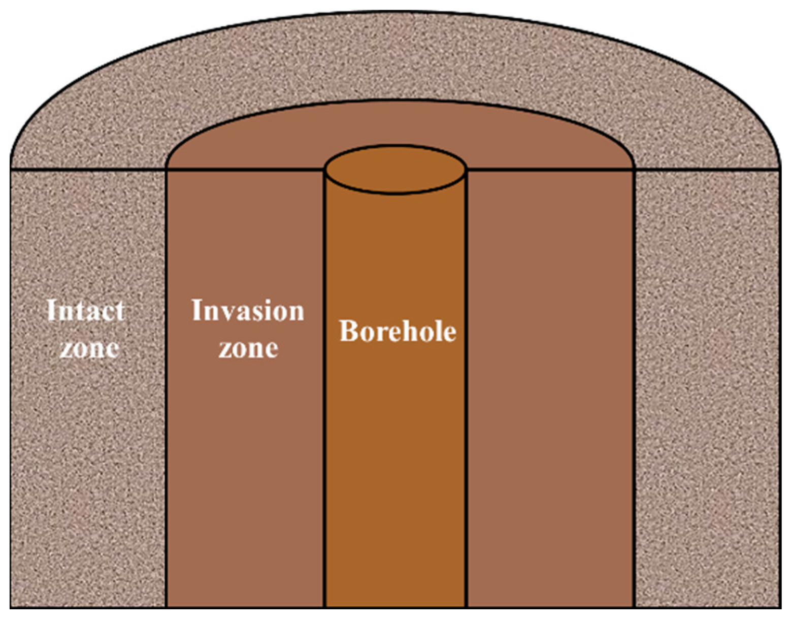
Figure 1. Some low-porosity and low-permeability rocks have dispersion frequency bands beyond 500 kHz [11].
Water 15 04213 g001
Figure 2. Schematic of single-transmission and dual-reception coil.
Water 15 04213 g002
Figure 3. Comparison of analytical and numerical solutions of: (a) EATT and (b) Δφ. ΔL is set to 5 cm, and L1 and L2 are set to 30 cm and 25 cm.
Water 15 04213 g003
Figure 4. Schematic of the three-layer medium model.
Water 15 04213 g004
Figure 5. Pseudo radial integral geometric factor changes with L1 at measurement frequencies and different DOI: (a) 0.3 m; (b) 0.5 m; (c) 1 m; and (d) 1.5 m. ΔL is set to 0.2 m, and the L1 corresponding to the intersection of the curve. The straight line when GΔφ(di) = 0.5 is the L1 that meets the design requirements.
Water 15 04213 g005
Figure 6. The three-layer formation model with a wellbore. The logging depth of the target layer center is 0 m.
Water 15 04213 g006
Figure 7. The response signals of the single-transmission dual-reception coil system to the three-layer formation model with different target layer thickness: (a) EATT and (b) Δφ. The DOI of the coil system is 0.5 m, and the measurement frequency is 8 MHz.
Water 15 04213 g007
Figure 8. The Δ φ curves of the single-transmission dual-reception coil systems with the DOI of 0.3 m to the three-layer formation model at different frequencies: (a) 0.25 MHz; (b) 0.5 MHz; (c) 1 MHz; (d) 2 MHz; (e) 4 MHz, and (f) 8 MHz.
Water 15 04213 g008
Figure 9. EATT curves to three-layer formation model at a frequency of 8 MHz of the single-transmission dual-reception coil systems with different DOI: (a) 0.3 m; (b) 0.5 m; (c) 1 m; (d) 1.5 m.
Water 15 04213 g009
Figure 10. Schematic diagram of the model when the recording point is located at (a) the top and (b) the bottom interfaces of the target layer.
Water 15 04213 g010
Figure 11. The measurement principle of the dual-transmission and dual-reception coil system.
Water 15 04213 g011
Figure 12. The response curves of the dual-transmission and dual-reception coil system to the three-layer stratum model: (a) EATT and (b) Δφ. In the model, the thickness of the low-resistance target layer is 2 m, and the reception coils spacing is 0.2 m.
Water 15 04213 g012
Table 1. Model parameters for the investigation of DOI of the coil systems.
ParametersBoreholeInvasion ZoneIntact Zone
Inner radius (m)00.054DOI
Outer radius (m)0.054DOI25
Relative magnetic permeability111
Relative permittivity755030
Conductivity (S/m)10.50.1
Table 2. Source-receiver distances for single-transmission dual-reception coil system corresponding to different measurement frequencies and DOI.
Frequency
(MHz)
DOI = 0.3 mDOI = 0.5 mDOI = 1 mDOI = 1.5 m
L1 (m)L2 (m)L1 (m)L2 (m)L1 (m)L2 (m)L1 (m)L2 (m)
0.250.080.280.330.531.181.382.372.57
0.50.110.310.410.611.491.692.883.08
10.160.360.530.731.832.033.343.54
20.230.430.690.892.152.353.633.83
40.320.520.861.062.362.563.783.98
80.420.621.021.222.472.673.834.03
Table 3. Parameters of the six-transmission dual-reception coil systems corresponding to different DOI.
DOI/mCoil System Structure
0.3T1-0.10-T2-0.09-T3-0.07-T4-0.05-T5-0.03-T6-0.08-R1-0.20-R2 (m)
0.5T1-0.16-T2-0.17-T3-0.16-T4-0.12-T5-0.08-T6-0.33-R1-0.20-R2 (m)
1T1-0.11-T2-0.21-T3-0.32-T4-0.34-T5-0.31-T6-1.18-R1-0.20-R2 (m)
1.5T1-0.05-T2-0.15-T3-0.29-T4-0.46-T5-0.51-T6-2.37-R1-0.20-R2 (m)
Table 4. Model parameters for the investigation of vertical resolution of the coil systems.
ParametersBoreholeTarget LayerSurrounding Layer
Inner radius (m)00.0540.054
Outer radius (m)0.0542525
Relative magnetic permeability111
Relative permittivity756530
Conductivity (S/m)10.0010.1
Disclaimer/Publisher’s Note: The statements, opinions and data contained in all publications are solely those of the individual author(s) and contributor(s) and not of MDPI and/or the editor(s). MDPI and/or the editor(s) disclaim responsibility for any injury to people or property resulting from any ideas, methods, instructions or products referred to in the content.

