Article

Flood Detection in Polarimetric SAR Data Using Deformable Convolutional Vision Model

1
School of Surveying and Land Information Engineering, Henan Polytechnic University, Jiaozuo 454000, China
2
Key Laboratory of Mine Spatio-Temporal Information and Ecological Restoration, Henan Polytechnic University Ministry of Natural Resources, Jiaozuo 454000, China
*
Author to whom correspondence should be addressed.
Water 2023, 15(24), 4202; https://doi.org/10.3390/w15244202
Submission received: 1 November 2023 / Revised: 28 November 2023 / Accepted: 30 November 2023 / Published: 5 December 2023
(This article belongs to the Special Issue Flood Monitoring, Forecasting and Risk Assessment)

Abstract

:
Floods represent a significant natural hazard with the potential to inflict substantial damage on human society. The swift and precise delineation of flood extents is of paramount importance for effectively supporting flood response and disaster relief efforts. In comparison to optical sensors, Synthetic Aperture Radar (SAR) sensor data acquisition exhibits superior capabilities, finding extensive application in flood detection research. Nonetheless, current methodologies exhibit limited accuracy in flood boundary detection, leading to elevated instances of both false positives and false negatives, particularly in the detection of smaller-scale features. In this study, we proposed an advanced flood detection method called FWSARNet, which leveraged a deformable convolutional visual model with Sentinel-1 SAR images as its primary data source. This model centered around deformable convolutions as its fundamental operation and took inspiration from the structural merits of the Vision Transformer. Through the introduction of a modest number of supplementary parameters, it significantly extended the effective receptive field, enabling the comprehensive capture of intricate local details and spatial fluctuations within flood boundaries. Moreover, our model employed a multi-level feature map fusion strategy that amalgamated feature information from diverse hierarchical levels. This enhancement substantially augmented the model’s capability to encompass various scales and boost its discriminative power. To validate the effectiveness of the proposed model, experiments were conducted using the ETCI2021 dataset. The results demonstrated that the Intersection over Union (IoU) and mean Intersection over Union (mIoU) metrics for flood detection achieved impressive values of 80.10% and 88.47%, respectively. These results surpassed the performance of state-of-the-art (SOTA) models. Notably, in comparison to the best results documented on the official ETCI2021 dataset competition website, our proposed model in this paper exhibited a remarkable 3.29% improvement in flood prediction IoU. The experimental outcomes underscore the capability of the FWSARNet method outlined in this paper for flood detection using Synthetic Aperture Radar (SAR) data. This method notably enhances the accuracy of flood detection, providing essential technical and data support for real-world flood monitoring, prevention, and response efforts.

1. Introduction

Floods, being among the most devastating natural disasters on a global scale, stand out as the most frequent and widespread natural calamities, exerting a severe impact on both human survival and economic progress [1]. The period spanning from 2000 to 2018 saw a staggering 913 major flood events worldwide, during which flooding directly affected an extensive land area of 2.23 million square kilometers and a human population ranging between 255 and 290 million individuals [2]. Evidently, floods have resulted in substantial losses in terms of global economic development and human lives. Therefore, the acquisition of timely and precise information regarding flooded regions holds paramount significance for the relevant authorities in crafting disaster relief strategies and conducting post-disaster loss assessments [3].
In recent years, with the rapid development of Radio Electronics Technology, Sensor Technology, Computer Technology, and Aerospace Technology, Remote Sensing Technology has found widespread applications in flood disaster monitoring [4]. Satellite remote sensing images offer advantages in providing macroscopic, objective, and timely surface information [5]. They can overcome the difficulties of inconvenient transportation and inaccessibility of submerged areas during disaster investigations, saving human and time costs. This makes them particularly suitable for large-scale, multi-level synchronous monitoring of flood disasters, offering a fast and cost-effective solution for flood monitoring. Several scholars have conducted research on how to use multi-temporal and multi-spatial remote sensing images to detect flood areas quickly and accurately. The Dartmouth Flood Observatory (DFO) has developed a global near-real-time mapping product for floods using MODIS data [6]. Lin et al. [7] analyzed the impact of flood basins on the environment using a long-time series of Landsat images, demonstrating that optical remote sensing images can be used for environmental analysis and planning for natural disasters. However, flood detection in medium to low-resolution optical images can be affected by terrain shadows. To address this issue, Lin et al. [8] proposed using digital elevation models (DEM) and other terrain data to remove terrain shadows, thereby improving the accuracy of flood detection. Large-scale and high-frequency observations using optical remote sensing images can monitor flood changes [9]. However, due to adverse weather conditions during flood events, optical sensors are sensitive to cloud cover and rainfall, making it challenging to obtain effective monitoring data during flooding [10]. Active microwave remote sensing [11] can address the emergency flood mapping problem during cloudy weather conditions. Martinis [12] developed the Visible Infrared Imaging Radiometer Suite National Oceanic and Atmospheric Administration George Mason University Flood Version 1.0 (VIIRS NOAA GMU Flood Version 1.0) using Suomi National Polar-orbiting Partnership (SNPP)/Visible Infrared Imaging Radiometer Suite (VIIRS) shortwave infrared data, enabling medium-resolution and frequent flood mapping. However, due to resolution limitations, these data cannot provide sufficient detail, leading to inaccuracies in pinpointing flood boundaries and capturing local variations in flood extents.
With the development of Synthetic Aperture Radar (SAR), SAR has gained significant attention for flood detection due to its unique wavelength characteristics. SAR has the capability to penetrate cloud and precipitation particles, making it immune to the influence of weather and time. It offers broad coverage and is particularly sensitive to water bodies [13]. Therefore, many researchers have been focusing on utilizing SAR images for flood detection. To date, flood extraction methods based on SAR images include threshold-based methods [14], object-oriented methods [15], active contour methods [16], and data fusion methods [17]. However, traditional SAR data-based flood monitoring methods face challenges when dealing with large areas due to issues such as speckle noise and uneven grayscale distribution in SAR images. In this context, the combination of SAR data with intelligent water extraction algorithms has become a hot topic.
To date, deep learning algorithms have achieved excellent results in various fields such as semantic segmentation [18], object detection [19], and image classification [20], providing a viable approach for flood detection. Deep learning methods have strong applicability in the process of extracting information from multi-band remote sensing images as they eliminate the need for complex feature selection [21]. With the emergence of large-scale datasets and computing resources, Convolutional Neural Networks (CNN) [22] have become the mainstream in visual recognition. Researchers like Long et al. [23] introduced a semantic segmentation method based on Fully Convolutional Networks (FCN), which addressed image segmentation at the semantic level and classified images at the pixel level. Ronneberger et al. [24] proposed a U-Net network with an encoder-decoder structure capable of fusing low-resolution and high-resolution features, thus improving the accuracy of image segmentation. Numerous classic semantic segmentation models have been developed globally to enhance the accuracy and performance of semantic segmentation, such as Deeplabv3 [25], UNet++ [26], and HRNet [27], among others. In recent years, the superior performance of deep learning has sparked immense interest in the hydrological community. Ng et al. [28] delve into the characteristics of deep learning models, the structure and features of hybrid models, and the crucial role of optimization methods. This provides the most recent snapshot of deep learning modeling applications in streamflow forecasting. The ANN3 model developed by Essam et al. [29] demonstrated strong adaptability and reliability, offering more precise water flow predictions to mitigate urban and environmental damages. In recent years, deep learning models have been gradually applied to water body extraction from remote sensing images. For instance, Chen et al. [30] utilized convolutional neural networks for water body extraction, demonstrating the effectiveness of deep learning methods in comparison to traditional methods like Normalized Difference Water Index (NDWI). He et al. [31] introduced an attention mechanism to adjust the feature weights in the hopping connection part of the U-net network and extracted the boundary information of alpine glacial lakes more accurately. Zhong et al. [32] introduced a two-way channel attention mechanism and a deep expansion residual structure to construct the MIE-Net network to improve the segmentation accuracy of the lake. Wang et al. [33] proposed a multiscale lake water body extraction network, particularly excelling in extracting small lake water bodies. Nemni et al. [34] devised a convolutional neural network for flood mapping, enabling fully automatic and rapid flood monitoring. Peng et al. [35] introduced a self-supervised learning framework for urban flood mapping, significantly enhancing the accuracy of urban flood monitoring. Yuan et al. [36] innovatively proposed the Enhanced Atrous Spatial Pyramid Pooling (EASPP) module, which maintains the saliency of high-dimensional features and improves the recognition ability of tiny water bodies. However, due to the diverse morphology and varying sizes of water bodies, there are limitations in the convolutional layers used in CNN models, particularly with regard to their limited receptive fields. This limitation makes it challenging to obtain accurate contextual information from the images, resulting in difficulties distinguishing between water bodies and shadows, incomplete extraction of small water bodies, and issues with river extraction. These limitations have restricted the application of water body extraction products.
The Transformer [37] is a deep learning model based on the self-attention mechanism, which has achieved significant success in natural language processing. Unlike CNN, the self-attention module of the Transformer Neural Network (TNN) can quickly model long-range feature relationships, allowing for the precise extraction of global features over a wide range. As a result, researchers have started exploring the application of transformer neural networks in image semantic segmentation tasks, with the Vision Transformer (ViT) [38] being the most representative model. ViT’s Multi-head Self-Attention (MHSA) module exhibits long-range dependencies and adaptive spatial aggregation. In addition to MHSA, transformer neural networks also include a range of advanced components not found in standard CNNs, such as Layer Normalization (LN) [24], Feed Forward Networks (FFN), GELU [25], and more. This enables ViT to learn more robust representations from a large amount of data compared to CNNs, leading to great success in visual tasks. Therefore, many researchers have applied TNN to hydrology. For example, Mustafa Abed et al. [39] established an evaporation prediction model based on the deep learning architecture of a transformer, which outperformed two DL models, namely Convolutional Neural Network and Long Short-Term Memory, in terms of prediction effect, indicating its application potential in hydrology. Donghui Ma et al. [40] proposed a Water Index and Swin Transformer Ensemble (WISTE) method for automatic water body extraction, which also achieved good segmentation results. However, despite its excellent performance in visual tasks, ViT’s global attention mechanism introduces expensive computational and memory complexity. This complexity can pose significant challenges, especially when dealing with high-resolution images. In addition, ViT’s ability to capture local information in relation to images is relatively weaker. In semantic segmentation tasks, these drawbacks can result in increased computational burdens when processing large-sized images and may not adequately capture pixel-level detail information, affecting the accuracy and the recognition capability of small structures during segmentation.
By comparing CNNs and TNNs, it can be found that: (1) Compared to TNNs with MHSA, the de-facto effective receptive field of CNNs [41] stacked by 3 × 3 regular convolutions is relatively small. Even with very deep models, the CNN-based model still cannot acquire long-range dependencies like ViTs, which limits its performance. (2) Compared to MHSA whose weights are dynamically conditioned by the input, since regular convolution has highly inductive properties, CNN models composed by regular convolutions might converge faster and require less training data than TNNs, but it also restricts CNNs from learning more general and robust patterns from web-scale data. As an extension of the DCN series, Deformable Convolutional v3 (DCNv3) made up for the deficiencies of regular convolution in terms of long-range dependencies and adaptive spatial aggregation, and DCNv3 inherits the inductive bias of convolution, making the model more efficient with fewer training data and shorter training time. In addition, because DCNv3 is based on sparse sampling, it only needs a 3 × 3 kernel to learn long-range dependencies, which is more computationally and memory efficient than methods such as MHSA and re-parameterizing large kernel [42] and is easier to optimize, avoiding extra auxiliary techniques used in large kernels.
The main contributions of the study are as follows:
(1)
Introducing the |VV|/|VH| Ratio to Enhance Data Features. Given the limitations of dual-polarized data in Sentinel-1, and the |VV|/|VH| ratio’s significant capability to enhance the reflective properties of water bodies, causing them to exhibit relatively higher pixel values in the ratio image. In this study, polarimetric data VV, VH, and |VV|/|VH|ratio, which was combined into an RGB image using band combination, was used as an input to the model, so that the model could better capture the reflectance change of the flood boundary.
(2)
The introduction of this method contributes to the improvement of the performance of flood detection models, enhancing their sensitivity to changes in the flood region.
(3)
A flood detection network model (FWSARNet) is proposed. In the encoder part, the FWSARNet model proposed in this paper introduced deformable convolution as the core operator, and deformable convolution (DCNv3) was used to replace the MHSA (Multi-Head Self-Attention) module in ViT, which could better capture the local details and spatial variations of the flood boundary present in the SAR image while reducing the parameters, thus, realizing the adequate extraction of local details and spatial variation features of the flood boundary.
(4)
In the decoder part, the model adopted the method of multi-level feature map fusion, which carried out multi-scale feature fusion and up-sampling operations on different levels of feature maps, combining different levels of feature information in the detection process could retain more semantic and detailed information, which further improved the recognition ability of fine water bodies.

2. Methods

Firstly, after completing the SAR image pre-processing, the Sentinel-1 dual-polarized images and the calculated |VV|/|VH| ratio images were combined into a new image containing three bands. Secondly, the obtained new images were divided into training dataset, validation dataset, and test dataset, and the data-augmented training dataset and validation dataset were input into the FWSARNet model for training. Finally, a variety of evaluation indicators were used to quantitatively evaluate the flood extraction accuracy of the FWSARNet model in the test dataset. The specific flowchart of this study is shown in Figure 1.
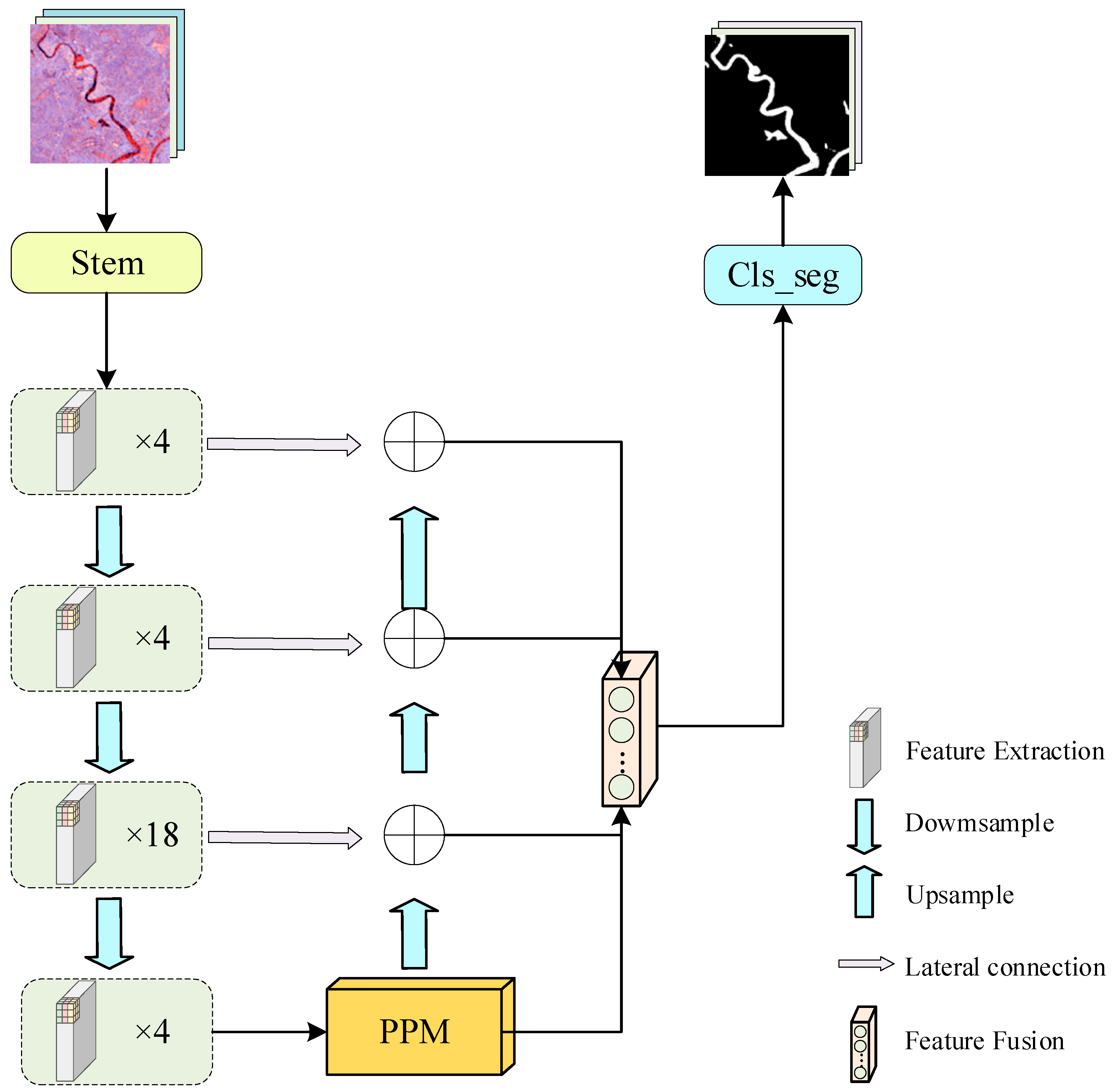
This study presents the flood detection network FWSARNet for Synthetic Aperture Radar (SAR) images, as depicted in Figure 2. The model is a convolution-based pyramid architecture, consisting of an encoder and a decoder. The encoder is composed of the convolutional stem layer, feature extraction module, and downsampling layer. The decoder consists of the Pyramid Pooling Module (PPM), upsampling layer, and feature fusion module. In this section, we will provide a detailed description of the proposed flood detection network FWSARNet.

2.1. Encoder

The FWSARNet model encoder consists of 1 convolutional stem (Stem layer), 4 sets of feature extraction modules, and 3 downsampling layers. Each set of feature extraction modules forms one stage, extracting features at a particular scale. The downsampling layers are distributed between the four stages, resizing the feature maps to different scales. Specifically, the feature extraction modules are responsible for feature learning, while the Stem layer and downsampling layers handle dimensionality reduction and upscaling. The encoder ultimately produces four scale-specific feature maps, denoted as X1, X2, X3, and X4.

2.1.1. Stem and Downsample Layers

The convolutional Stem layer and the downsampling layers play a crucial role in the encoder. The Stem is responsible for the initial processing of input data. As shown in Figure 3, it consists of two convolutional layers, two Layer Normalization (LN) layers, and one GELU layer. Each of the convolutional layers has a kernel size of 3, a stride of 2, and a padding of 1. Both convolutional layers are connected to Layer Normalization (LN) layers, which accelerates the model’s learning process, extracting fundamental features from the input SAR data as a foundation for further processing. The downsampling layers are strategically placed between two stages of feature extraction in the encoder. Their primary function is to reduce the spatial dimension of feature maps to capture features at different scales effectively, allowing the model to learn high-level and low-level features. Additionally, the downsampling layers contribute to improved computational efficiency and reduced model complexity. Similarly, the downsampling layers consist of 3 × 3 convolutions with a stride of 2 and padding of 1, followed by an LN layer. The downsampling layers can be represented using the following formula.
X = L N ( C o n V 2 d ( X ) ) .

2.1.2. Feature Extraction Module

The Feature Extraction Module is designed by combining a Deformable Convolutions Network (DCN) [43] with a series of customized blocks and architectures similar to a transformer neural network. Unlike the traditional Multi-Head Self-Attention (MHSA) modules, the Feature Extraction Module is built upon Deformable Convolutions Network v3 [44] (DCNv3). As shown in Figure 4, each Feature Extraction Module block consists of a LayerNorm (LN), DCNv3, residual connections, and a Multilayer Perceptron (MLP) with a GELU non-linearity, the core operator is DCNv3. For other components, we adopted a pre-normalization setting and followed a design similar to a standard Transformer. Based on this design, the Feature Extraction Module can be represented as follows:
X ^ l = d r o p o u t γ × D C N L N X l 1 + X l 1 ,
X l = d r o p o u t γ × M L P L N X ^ l + X ^ l ,
where X ^ l and X l represents the outputs of the DCN module and the MLP module, respectively.
DCNv3 introduces learnable offsets to adjust the sampling positions of convolutional kernels, giving the convolution kernels the ability to deform spatially. This enables them to adaptively capture feature information from different locations, making them more suitable for variations in the shape and spatial changes of targets. DCNv3 addresses the shortcomings of traditional convolution in terms of long-range dependencies and adaptive spatial aggregation. Furthermore, as shown in Figure 5, DCNv3 draws inspiration from the concept of depth-wise separable convolution to reduce the complexity of the DCN operator. It also incorporates multiple sets of mechanisms and normalization modulation scalars. This achieves sparse global modeling while appropriately retaining the inductive bias of CNN, striking a better balance between computational efficiency and accuracy. DCNv3 can be represented as follows:
y p 0 = g = 1 G K = 1 k w g m g k x g p 0 + p k + Δ p g k ,
where G represents the number of groups. For the g group, w g represents the shared projection weights of that group, m g k ∈ R represents the modulated scalar at the k-th sampling point in group g normalized by the softmax function along dimension k, x g represents the sliced input feature map, and Δ p g k represents the offsets corresponding to grid sampling positions in the g group.

2.2. Decoder

The decoder in the FWSARNet model is responsible for taking the multi-scale features generated by the encoder and further processing them to produce the final flood detection results. It consists of three essential components: the Pyramid Pooling Module (PPM), the upsampling layers, and the feature fusion module.

2.2.1. Pyramid Pool Module

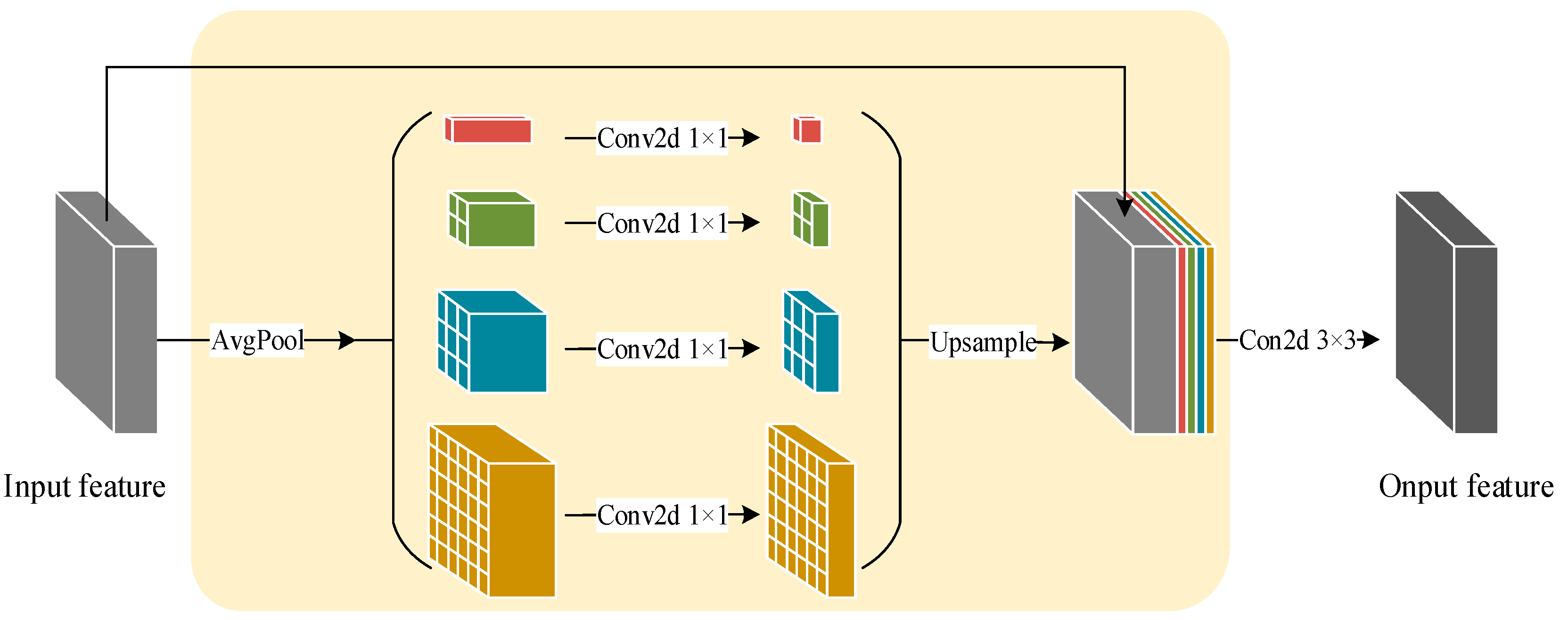
The Pyramid Pooling Module (PPM) [45] fuses multi-scale features by performing pooling operations on feature maps at different scales. It consists of multiple branches, each with a different pool size. These branches aid in extracting features at different scales and combining them to enrich the feature representation, providing a more comprehensive contextual understanding of the input data. By introducing the PPM, our model could better perceive variations in object scales, leading to improved segmentation accuracy and detail preservation.
As illustrated in Figure 6, we applied average pooling at different scales to the input feature map (512 × 8 × 8), resulting in feature maps of sizes 1, 2, 3, and 6. These feature maps were integrated using 3 × 3 convolutions and then upsampled to match the size of the input feature. They were concatenated along the channel dimension, including the original feature map. The concatenated feature map had a size of 2560 × 8 × 8, and a final 3 × 3 convolution was applied to produce a composite feature map that combined information from various scales. This feature map had the same size as the input (512 × 8 × 8). This process aimed to balance global semantic information and local detail information. This process can be mathematically expressed as follows.
X u p i = U P ( B N ( C o n v 2 d ( A v g P o o l ( X 4 ) ) ) ) ,
X P P M = C o n v 2 d ( C o n c a t ( I n p u t , X u p i ) ) ,
where i = 1, 2, 3, and 4, and UP indicates the up-sampling operation. X u p i is the upsampled output result,   X 4 is the output feature of the fourth stage of the encoder, and X P P M represents the output of the Pyramid Pool Module.

2.2.2. Feature Fusion Module

The top-level feature maps obtained through the Pyramid Pool Module contained rich semantic information, but they had lower resolution, especially near the flood boundaries, and their resolution was not sufficient for accurate semantic predictions. However, the lower-level feature maps connected laterally and fused with their corresponding layers had low-level semantic information but higher resolution. To address this issue, the proposed network in this paper used a feature fusion module to combine feature maps from different layers, effectively capturing multi-scale and multi-level semantic information, thereby improving flood prediction performance. As shown in Figure 7, first, feature maps from different layers were individually subjected to a 3 × 3 convolution for feature integration. Then, the high-level features were upsampled, and these feature maps were fused along the channel dimension to obtain a feature map with multi-level features. This process can be represented using the following equation.
X u p i = U P ( B N ( C o n v 2 d ( X i ) ) ) ,
O u t p u t = C o n v 2 d ( C o n c a t ( X 4 X u p i ) ) ,
where i = 1, 2, and 3, X i represents the three high-level features, UP denotes the upsampling operation, X u p i represents the result after upsampling, and O u t p u t represents the result after feature fusion and a 3 × 3 convolution for feature integration.

2.3. Experimental Metrics

Through a comprehensive consideration of the research in related fields [40,46], we selected five widely used evaluation metrics, namely Intersection over Union (IoU), mean Intersection over Union (mIoU), precision (P), recall rate (R), and F1-score as evaluation metrics. IoU and mIoU were used to evaluate the performance of the model in terms of target spatial positioning and boundary accuracy, while the precision and recall rate was used to evaluate the ability of the model to accurately predict the flood area and successfully identify the real flood area for the flood detection task. The F1-score, as a harmonic average of precision and recall, provided an overall assessment of the balance between the accuracy and completeness of the model. By selecting these five metrics, we ensured a comprehensive evaluation of the model’s performance in all aspects of the flood detection task.
The Intersection over Union (IoU) calculates the ratio of the intersection of the true values and predicted values to their union. This ratio can be expressed as the intersection (TP) divided by the sum of (TP, FP, and FN). The formula for calculating IoU is as follows:
I o U = T P F P + F N + T P .
The mean Intersection over Union (mIoU) is the average IoU computed for each class. The formula for calculating mIoU is as follows:
M I o U = 1 K + 1 i = 0 k T P F P + F N + T P .
Precision, also known as positive predictive value, is a metric that measures the probability of true positive samples among all the samples predicted as positive. The formula for calculating precision is as follows:
P = T P T P + F P .
Recall, also known as sensitivity or true positive rate, is a metric that measures the probability of samples correctly identified as positive among all the actual positive samples. The formula for calculating recall is as follows:
R = T P T P + F N .
The F1-score can comprehensively consider the precision rate and recall rate to make it more representative.
F 1 = 2 × P r e c i s i o n × R e c a l l P r e c i s i o n + R e c a l l .
In the above equation, TP represents the number of samples belonging to the “flood” category correctly identified as “flood” by the system, FP represents the number of samples belonging to the “background” category mistakenly classified as “flood” by the system, and FN represents the number of samples belonging to the “flood” category wrongly classified as “background” by the system.

3. Experiments

3.1. Dataset and Preprocessing

The dataset used in the experiments was derived from the ETCI 2021 flood dataset, which consists of SAR (Synthetic Aperture Radar) images captured by the European Space Agency’s Sentinel-1 satellite. These images were acquired in interferometric wide mode with a resolution of 5 × 20 m. The dataset included a total of 54 GeoTIFF format images, with a combined file size of 5.3 G. These images were divided into 256 × 256-pixel image patches, capturing both VV and VH polarization modes. Furthermore, the dataset provided annotations for pre-flood water pixels and flood-labeled pixels during flood events. The dataset covered a diverse range of regions, including Nebraska, North Alabama, Bangladesh, Florence, and more, encompassing five different flood events in various settings, such as agricultural land and urban environments. This diversity allowed the dataset to effectively reflect a wide range of changes in regions affected by floods.
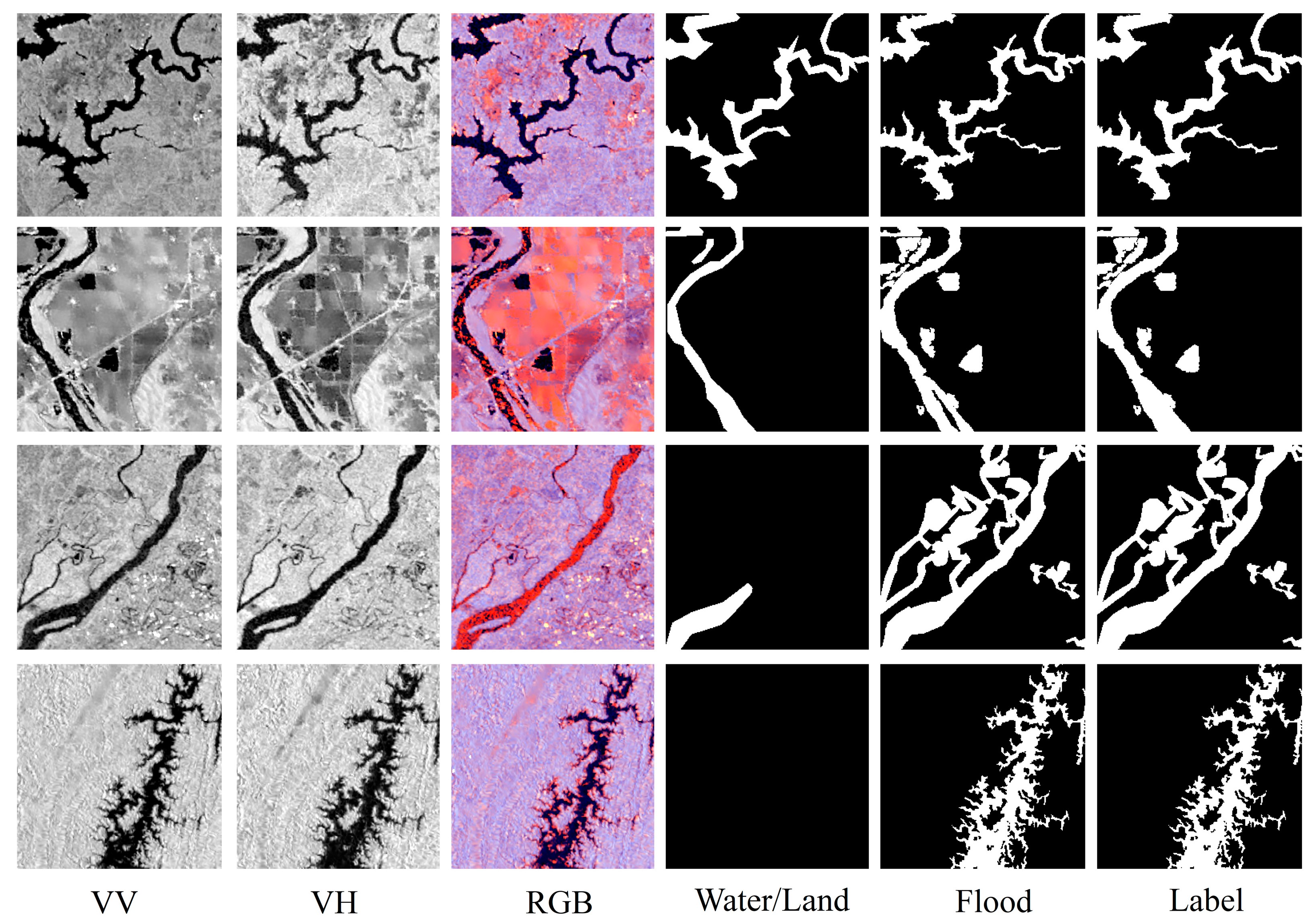
The data preprocessing workflow was as follows: (1) To remove speckle noise from SAR images, a Lee filter with a window size of 5 × 5 was applied. This filtering process helps in improving the quality of SAR images and is chosen for its balance between noise reduction effectiveness and processing speed. (2) Considering the limited polarization data from Sentinel-1 and the enhancement of water features using the |VV|/|VH| ratio, the |VV|/|VH| ratio was introduced to enrich the model features. In this study, a composite RGB dataset was created using the red channel for VV, the green channel for VH, and the blue channel for |VV|/|VH| ratio (as shown in Figure 8). (3) The labeled water pixels and flood pixels were combined to create the label data used during the training process. (4) Some images in the dataset contained striping artifacts or were completely empty, which can introduce noise. To improve the quality and reliability of the training data, images with an area smaller than 0.5% were excluded during training. (5) Data augmentation was performed to obtain a sufficient number of samples and prevent overfitting during model training. Data augmentation included random rotations, random cropping, horizontal flipping, and optical distortions applied to both the images and their corresponding label images.

3.2. Model Training

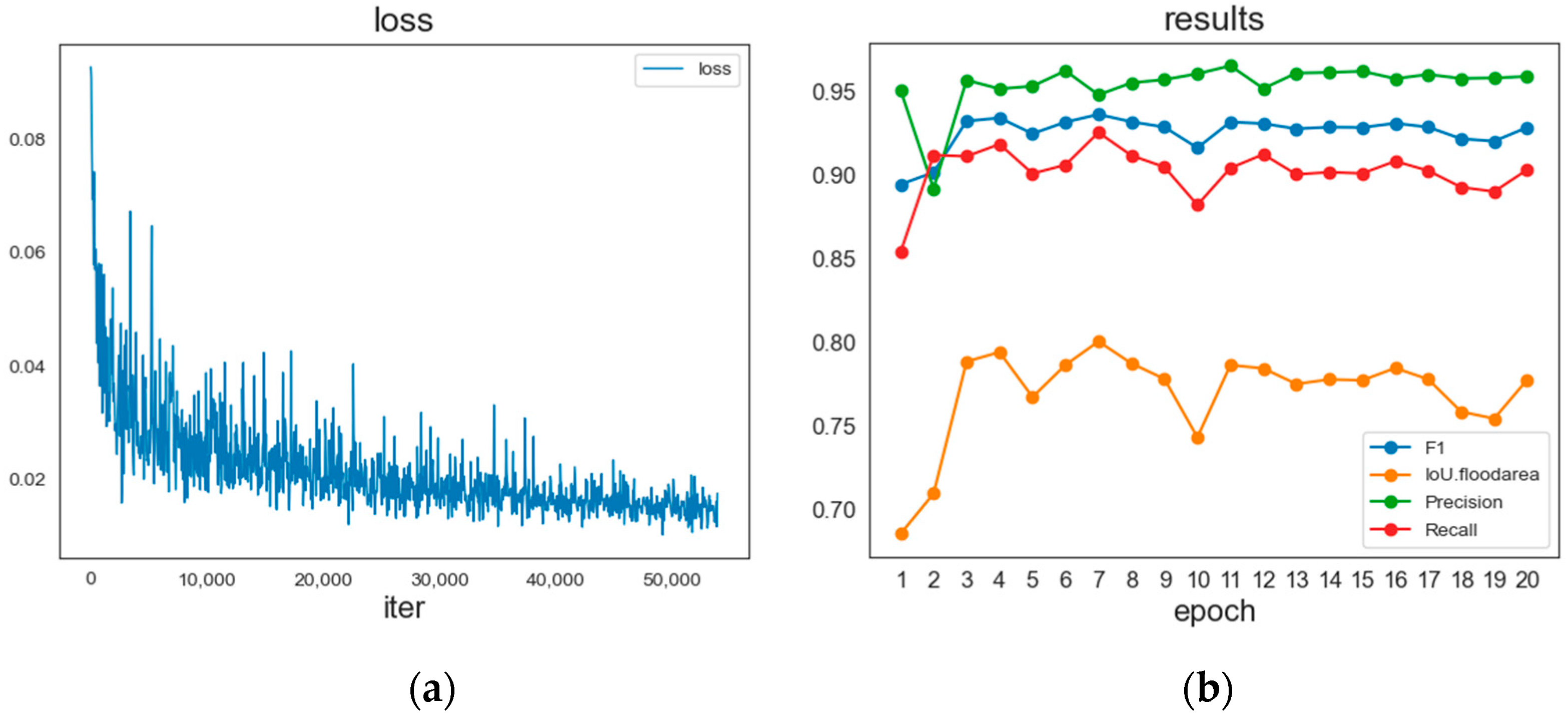
Due to the substantial computational requirements and numerous parameters in deep learning, the experimental setup demands meticulous attention. This study conducted thorough configurations in both hardware and software environments to ensure the reliability and performance of the experiments. In terms of hardware, the experiments were carried out on a system running the Windows 10 operating system. The hardware configuration included 64 GB of RAM, an Intel Core i9-9900K processor, and an NVIDIA GeForce RTX 2080 graphics card with 8 GB of VRAM. These specifications were chosen to leverage the computational power needed for deep learning tasks. Regarding software, the experiments were conducted using Python 3.8 as the primary programming language. The model was implemented using the Pytorch deep learning framework. To harness the hardware’s full potential, GPU acceleration technology was employed. Hyperparameter tuning was a crucial aspect of the experiment. Through multiple iterations, this study established appropriate hyperparameter settings. Specifically, the number of training iterations was set to 20, the batch size was configured as 4, and the AdamW optimizer was used. The initial learning rate was defined as 6 × 10⁻⁵, with momentum parameters (betas) set to (0.9, 0.999), and a weight decay parameter of 0.01 was applied. Additionally, the cross-entropy loss function was used during the model training process. After several rounds of iterative training, the model ultimately achieved the desired state of convergence. These carefully considered hardware and software configurations, along with optimized hyperparameters, ensured both the reliability and high-performance execution of the experiments. Figure 9 shows the training loss curve and the evaluation index curve of the model.

3.3. Results

3.3.1. Optimizer Analysis

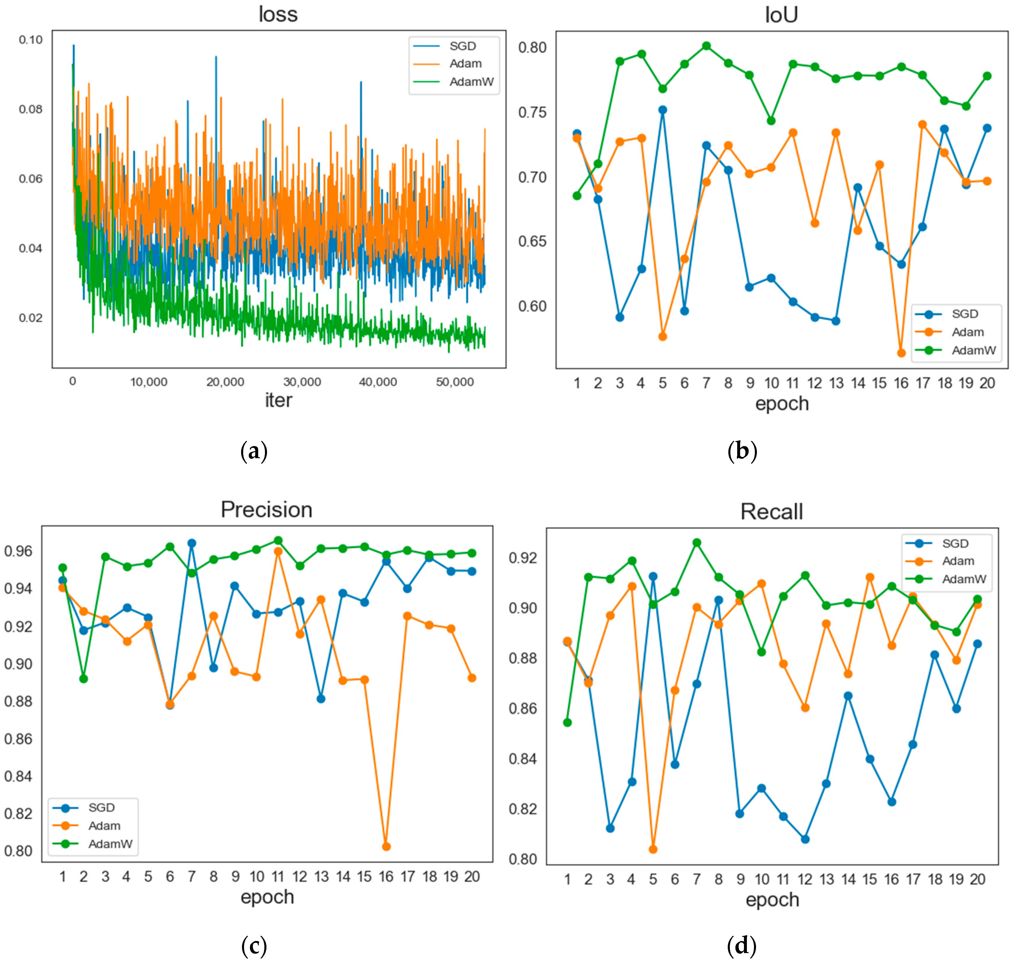
The essence of training a Convolutional Neural Network (CNN) is to continuously update parameters during the training process to minimize the loss. Currently, most optimization algorithms are achieved through iterations, primarily by optimizing a loss function to find the optimal parameters. To obtain a suitable optimizer, we experimented with different optimizers, including SGD, Adam, and AdamW, to analyze the training loss of the model.
Stochastic Gradient Descent (SGD) [47] is currently the most fundamental iterative algorithm for optimizing neural networks. It computes the derivatives of the error, with respect to the weights, layer by layer using the gradient descent method and then updates the weights and biases of the neural network layer by layer. SGD is known for its simplicity and ease of implementation, but it has some drawbacks, including relatively slow convergence and the potential for oscillations around saddle points. Its formula is as follows:
g t = l o s s ω t ,
ω t + 1 = ω t + l r × g t ,
where gt is the gradient of the loss function at time t with respect to the current parameter, ωt is the weight at time t, lr is the learning rate, and ωt+1 is the weight at time t + 1.
The Adaptive Moment Estimation (Adam) optimizer [48] is an adaptive optimization algorithm that adjusts the learning rate based on historical gradient information. Furthermore, it allows for the adaptation of momentum parameters to balance the influence of the previous and current gradients on parameter updates, preventing premature convergence to local minima. Additionally, the Adam optimizer normalizes parameter updates, ensuring that updates for each parameter have similar magnitudes, thereby improving training effectiveness. Finally, it incorporates L2 regularization to regularize the parameters, preventing overfitting of the neural network to the training data. Its formula is as follows:
m t 1 = m t 1 β 1 τ ,
v t 2 = v t 1 β 2 τ ,
ω t + 1 = ω t l r × m t 1 v t 2 ,
where m t 1 is to correct the deviation of first-order momentum, and v t 2 is to correct the deviation of second-order momentum, β1, β2 ∈ [0, 1].
The AdamW optimizer [49], proposed by Loshchilov and others, addresses a perceived issue with the traditional Adam optimizer combined with L2 regularization. It was observed that, under normal circumstances, larger weights should be penalized more, but Adam does not follow this principle. Therefore, the authors introduced the concept of weighted decay to create the optimized AdamW algorithm. AdamW retains the efficiency and low memory footprint of the Adam algorithm while improving its overall performance. This enhancement helps overcome potential issues with Adam, such as non-optimality and slow convergence. The parameter update formula for the optimization algorithm is as follows:
ω t + 1 = ω t η t α υ t + ε m t + λ · ω t ,
where t represents the time step, α represents the learning rate, ω t+1 represents the parameters to be updated, mt and vt represent the first-order moment momentum and second-order moment momentum respectively, λ represents the weight decay rate of each step, η t is a custom step size scale factor, and ε is an extremely small number to prevent the denominator from being 0.
Figure 10a illustrates the training losses when using three different optimizers. It is evident from the graph that SGD and Adam exhibited higher fluctuations in training loss, and the loss values were larger. In contrast, AdamW showed smaller fluctuations in training loss, resulting in smaller loss values. Figure 10b–d represents the IoU, precision, and recall on the validation dataset when using the three optimizers. It is evident from the figures that the AdamW optimizer outperformed the other optimizers across all three performance metrics. In addition, the results of Llugsi et al. [50] also showed that the AdamW optimizer had higher performance. Therefore, AdamW was selected as the network optimizer in this study.

3.3.2. Comparison of Different Backbone Models

To validate the effectiveness of different backbone architectures for water feature extraction in the FWSARNet model, this section provides a detailed comparison of various backbone architectures. These architectures include ResNet [41] based on convolution and residual connections, the Transformer-based Vision Transformer (ViT) [38], Twins_svt [51], and Swin Transformer [52]. All experiments maintained consistency by using the same decode_head structure. Evaluation metrics included Intersection over Union (IoU), mean IoU (mIoU), F1-score (F1), Precision, and Recall. Table 1 presents the prediction results of different backbones on the ETCI 2021 dataset, with the best results highlighted in bold for emphasis.
The results indicated that: (1) By observing the IoU and mIoU metrics, it was evident that the FWSARNet model achieved 80.06% and 88.49%, respectively, which were significantly better than other backbone models. This highlights the significant advantage of the FWSARNet model’s backbone in terms of the accuracy of water segmentation, enabling it to more precisely capture water features. (2) F1 scores are an important indicator of the balance between accuracy and recall. The network backbone of the model proposed in this paper also achieved the highest F1 score, reaching 93.68%, which showed that it could maintain a high recall rate while maintaining high precision. This conclusion was also verified by Precision and Recall scores, which were crucial for the accurate extraction of water features. (3) Furthermore, when compared to other network models, the FWSARNet model exhibited the highest improvements in terms of IoU and mIoU, which increased 11.89% and 7.03%, respectively. Even when compared to the high-performing backbone networks like Twins_svt and Swin Transformer, the IoU of the FWSARNet model was still 2–3 percentage points higher.
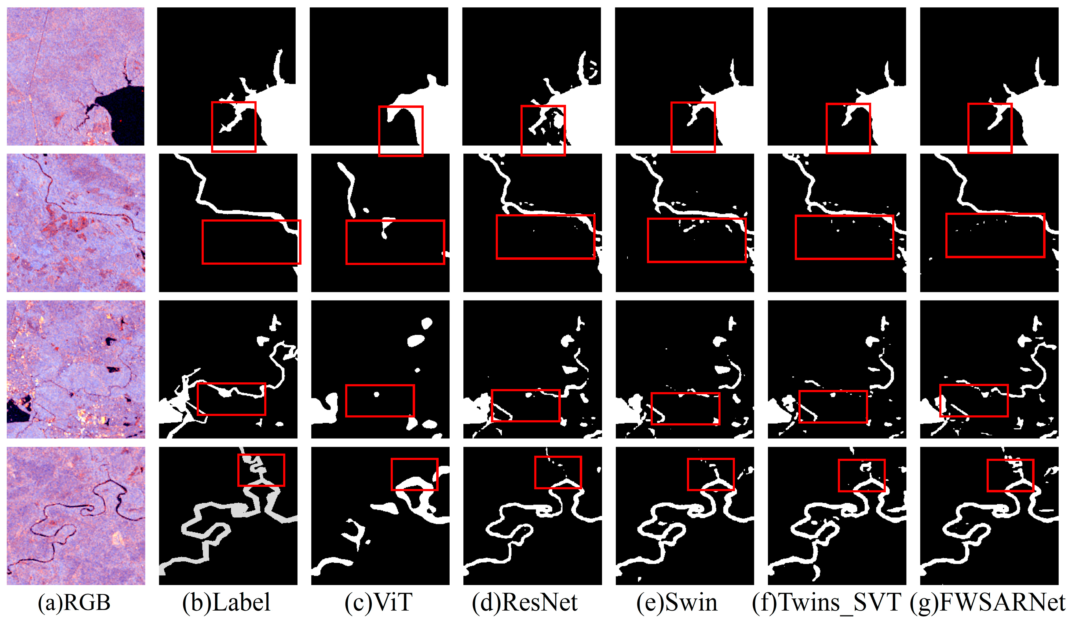
Figure 11 illustrates the visual results of flood detection using different backbone models on the ETCI 2021 test dataset. Observations from the results were as follows: The ViT model excels in modeling global context through its self-attention mechanism; however, its performance heavily relies on large-scale training data [38]. In ViT models, the relatively large receptive field leads to excessive averaging of details. Additionally, the fixed-size tokens are not well-suited for certain visual applications [51]. Consequently, in flood detection tasks, ViT’s performance was not ideal, as shown in Figure 10c, where the model could only detect large bodies of water and failed to accurately identify small rivers and flood boundaries. In contrast, the convolutional operations in ResNet are more flexible in handling different-sized receptive fields, making them better suited for tasks involving complex water boundaries. The spatially separable self-attention (SSSA) technique in Twins_svt can enable cross-group information exchange, aiming to reduce model complexity while improving accuracy. The Swin Transformer achieves significant results in image classification, object detection, and semantic segmentation by replacing the standard MHSA module in the Transformer block with the Shifted Window based Self-Attention (SW-MSA) technique, introducing connections between adjacent non-overlapping windows in the previous layer. Figure 11d–f shows that ResNet, Twins_svt, and Swin Transformer models performed well in flood detection. However, as shown in the third and fourth rows of Figure 11, they exhibited weaker performance in detecting small rivers and small water bodies. Furthermore, Figure 11d,e reveal that the ResNet and Swin Transformer models introduced considerable noise in flood detection. In comparison, Figure 11g demonstrates that the FWSARNet model excelled in flood detection by extracting the most comprehensive river and flood boundary details. It also performed better in detecting small rivers, producing results that were closely aligned with the ground truth labels. These findings were consistent with the results presented in Table 1.
In summary, the backbone network of the FWSARNet model exhibited the best performance, with the highest IOU, MIOU, Recall, and F1 metrics, with Precision being slightly behind Twins_svt. Visual results also demonstrated that the FWSARNet model performed exceptionally well. Therefore, the experimental results confirmed that replacing the Multi-Head Self-Attention (MHSA) module in ViT with deformable convolution DCNv3 better facilitates the comprehensive extraction of local details and spatial variations in flood boundaries.

3.3.3. Comparison of Different Decoder Models

For the flood detection task, we also experimented with different decode_head models, including Atrous Spatial Pyramid Pooling (ASPP) [53], Depthwise Separable Spatial Pyramid Pooling (DSASPPHead) [25], Feature Pyramid Network (FPN) [54], and Segformer [55] designed for the TNN architecture. Table 2 presents the prediction results of these different decode_head models on the ETCI 2021 dataset.
Based on Table 2, the comprehensive performance of different segmentation heads was compared and analyzed according to the performance indexes in the table. First of all, by observing the IoU and mIoU indicators, it can be clearly seen that the FWSARNet model exceeded other models when the IoU reached 80.1% and mIoU reached 88.47%, showing it had significant advantages in the accuracy of water body segmentation. Secondly, the FWSARNet model achieved a 93.67% F1 score, which was higher than other models, indicating that the model maintained a high recall rate while maintaining high precision, which is of great significance for the accurate extraction of water features. Comparing the performance of different segmentation heads, it was found that DSASPP, FPN, and Segformer performed well in IoU, mIoU, F1 scores, etc., but were slightly inferior to the FWSARNet model. In addition, in terms of Precision and Recall, the FWSARNet model also achieved a relatively high performance, 94.84%, and 92.59% respectively, indicating that the model could better balance accuracy and recall rate in practical applications.
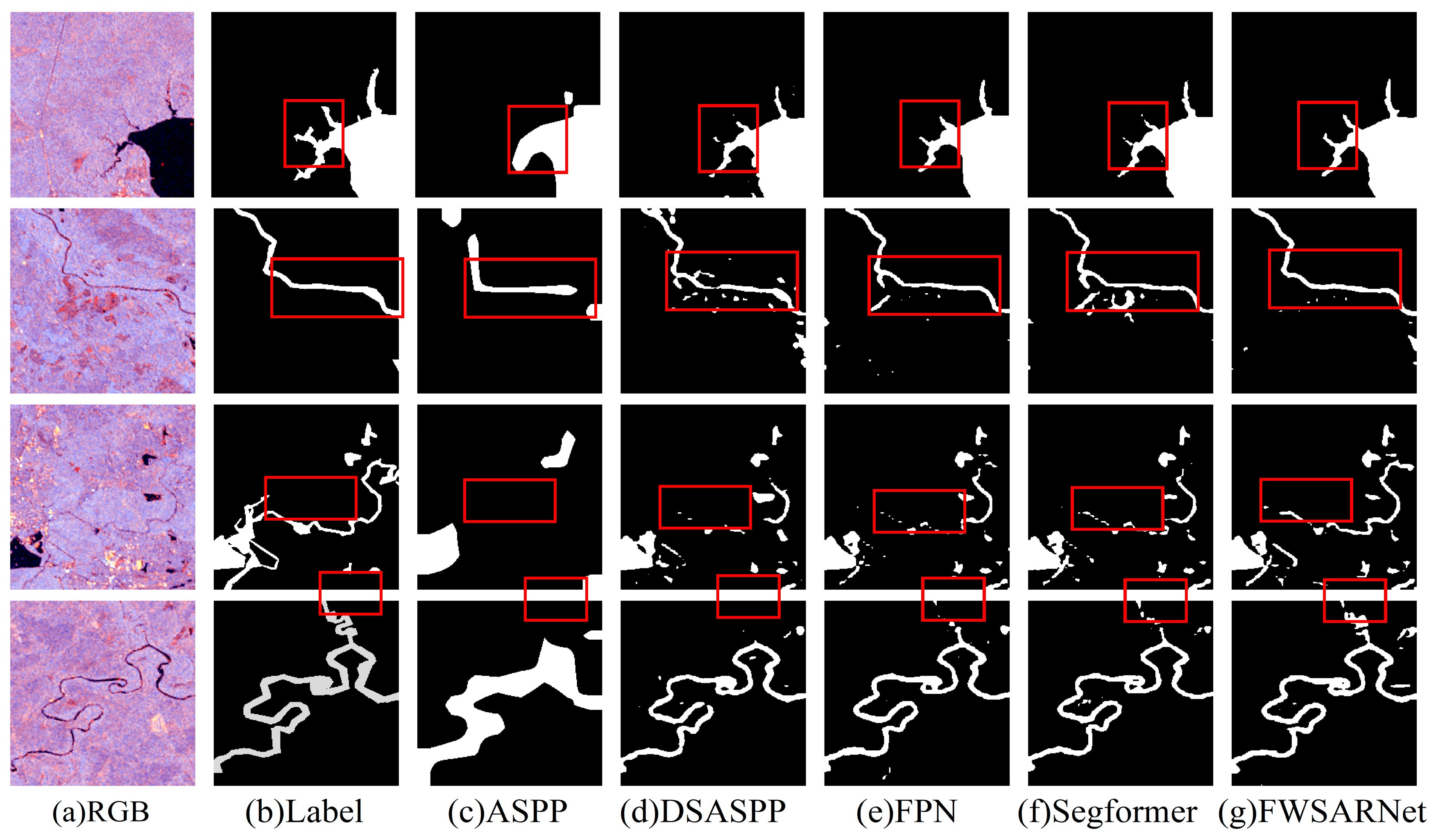
Figure 12 shows the visual results of different segmentation head models for flood detection on the ETCI2021 test dataset. The results of the model that used ASPP as the solution header can be seen in Figure 12c. Since ASPP mainly focuses on multi-scale context information, it could not make full use of local details for accurate river detection. Therefore, the model had a poor water detection effect, could only detect a large range of water, and could not accurately detect the water boundary. Figure 12d shows the detection effect of models using DSASPP as the decoder. On the basis of ASPP, DSASPP decomposes the standard convolution operation into depthwise convolution and pointwise convolution, which improves the efficiency and the segmentation accuracy. As shown in Figure 12d, the model with DSASPP as the segmentation head had a significant improvement in detection effect compared with ASPP, but it still could not detect tiny rivers and misdetected shadows for water bodies, resulting in more noise. By constructing a feature pyramid, FPN extracts features from networks at different levels and fuses these features to improve segmentation accuracy. As shown in Figure 12e, the model with FPN as the segmentation head could detect flood boundaries to a large extent, but the segmentation effect of small targets was insufficient, and small rivers could not be accurately detected. As shown in Figure 12f, the model Segformer was a semantic segmentation solution dock commonly used in TNNs, and the accuracy of the model depended on the self-attention mechanism of the transformer, which made it easy to recognize the mountain shadow as a water body in flood detection, and had a high error detection rate, and there were many breakpoints in the identification of small rivers. In contrast, Figure 12g shows that the decoder of the FWSARNet model could extract the most complete river information and flood boundary details in flood detection, and the detection effect was better for tiny rivers. This was consistent with the results in Table 2.
In summary, the solution terminal of the FWSARNet model had the best performance, with the highest indexes of IoU, mIoU, Recall, and F1, and the Precision had also reached an excellent level. The visualizations also showed that FWSARNet models performed best. Therefore, according to the experimental results, it can be proved that the multi-level feature map fusion method could further improve the recognition ability of small water bodies. Taking the above experimental results into consideration, the FWSARNet model showed excellent performance under several evaluated indexes and has the potential to become a cutting-edge model in the field of flood detection.

4. Discussion

4.1. Analysis of Data Category Weights

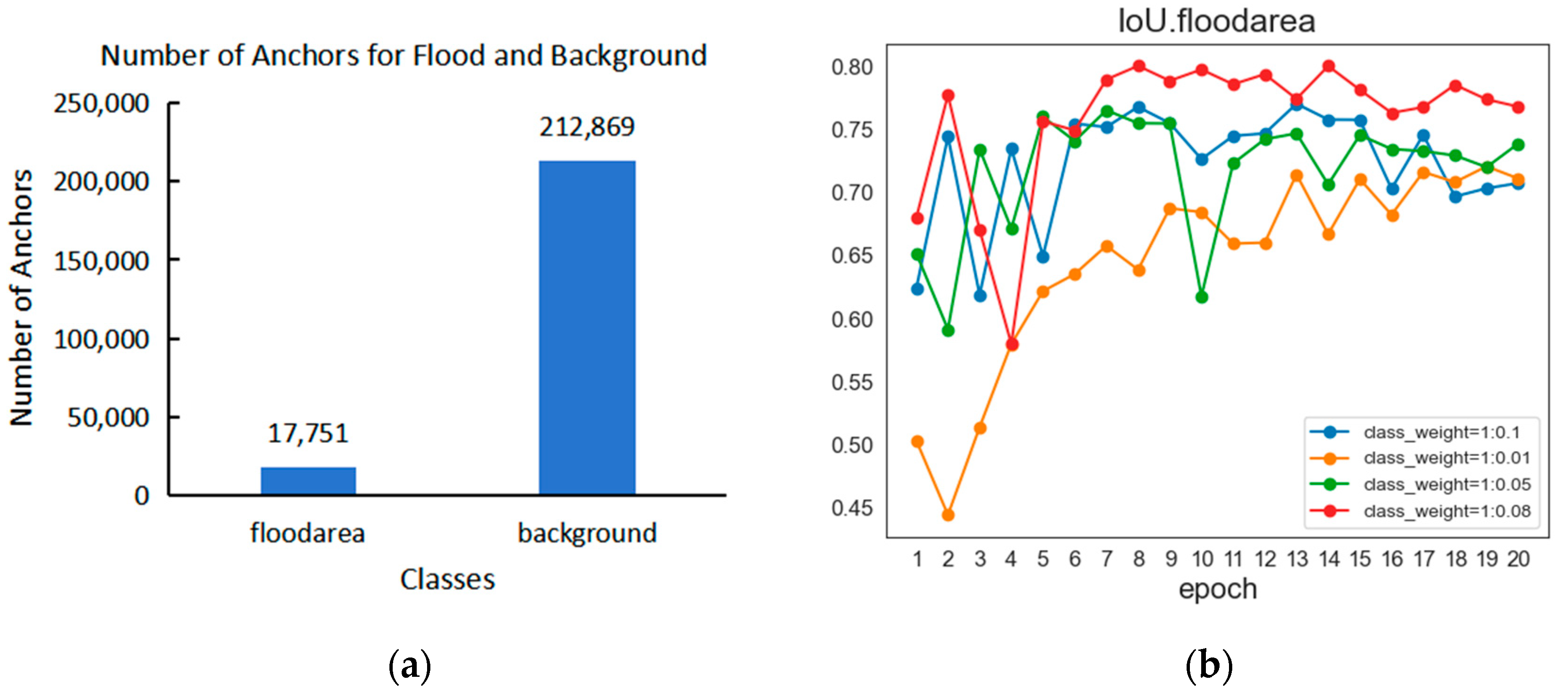
During the model training process, there was an issue of an imbalanced distribution of the number of foreground and background pixels. Specifically, the number of pixels in the flood-affected areas in the images was significantly less than the number of background pixels. As indicated by the pixel count data in Figure 13a, the number of pixels in the flood-affected areas was 17,751, accounting for only approximately 8% of the total number of pixels in the image. This imbalance may have a significant impact on the accuracy and robustness of the segmentation results.
To effectively address this issue, this study employed a category-weight adjustment strategy based on pixel values to weight the various pixel categories in the training dataset. Specifically, by analyzing the number of samples for each category in the training set, corresponding weights were introduced for different pixel categories. When a category had a larger number of samples, its weight was relatively lower. Conversely, categories with fewer samples received higher weights. The main objective of this weight adjustment strategy was to balance the model’s focus on different pixel categories, thereby enhancing the performance and robustness of the flood detection model. Considering that flood region pixels constituted only around 8% of the total image pixels, this experiment attempted various flood-to-background class weight ratios, including 1:0.1, 1:0.08, 1:0.05, and 1:0.01. The experimental results revealed that, as shown in Figure 13b, when the flood-to-background class weight ratio was set to 1:0.08, the model exhibited the most superior performance.

4.2. Model Efficiency Analysis

To enable a comprehensive assessment of the model’s complexity, we conducted an in-depth analysis of its computational efficiency. This analysis involved a meticulous comparison of the parameter calculations across different models. The results are presented in Table 3, which showcases the metrics for Floating Point Operations per Second (FLOPs), model parameters (Params), test time, and train time for various models assessed using the ETCI2021 dataset. Floating Point Operations per Second (FLOPs) indicates the number of floating point operations performed per second. In deep learning, FLOPs are often used to measure the computational complexity of a neural network model. The calculation method of FLOPs depends mainly on the different layer types in the network. For the Convolutional Layer, FLOPs can be calculated by the size of the convolutional kernel, the size of the input feature map, and the size of the output feature map. For a convolutional layer with a convolutional kernel size of (Kh, Kw), an input feature map size of (Hin, Win), and an output feature map size of (Hout, Wout), FLOPs are calculated as follows:
F L O P s = K h × K w × C i n × C o u t × H i n × H o u t ,
where Cin and Cout are the number of input and output channels, respectively. For the Fully Connected Layer, also known as the linear layer, the calculation of FLOPs can be determined by the input feature dimension (Din) and the output feature dimension (Dout). FLOPs are calculated as follows:
F L O P s = D i n × D o u t ,
Since there are no parameters to be learned for the pooling layer, the calculation formula for FLOPs is usually simpler, for the pooling layer with a feature map size of H × W, the number of channels is C, and the stride length is s, the calculation formula for FLOPs is as follows: maximum pooling is like Equation (22), and average pooling is like Equation (23).
F L O P s = H s × W s × C ,
F L O P s = 3 × H s × W s × C ,
In addition, for Activation Functions, such as GULE in the model, the calculation of FLOPs is generally considered to be small and usually negligible.
Table 3 reveals a compelling performance advantage of our FWSARNet in terms of FLOPs and model parameters (Params). Remarkably, FWSARNet stands out with only 58.75 G FLOPs and 58.96 M model parameters. This implies that FWSARNet achieved outstanding performance with remarkably low computational complexity, a highly valuable trait for practical applications. Furthermore, it is crucial to assess the practicality of a model by considering test and train times. In this context, the FWSARNet model excelled, achieving optimal results with test and train times of 140 s and 263.23 min, respectively. These metrics highlight the real-time capabilities and efficiency of FWSARNet in practical applications. In contrast, models such as ResNet, Twins_svt, and SwinTransformer exhibited good accuracy but came with higher computational complexity. The ViT model, on the other hand, fell short in terms of accuracy and presented a notable computational burden. Collectively, these results demonstrated that our proposed method incurs the lowest computational cost and is notably more efficient than alternative models.

4.3. Comparison with Other SOTA Models

When comparing the FWSARNet model to other state-of-the-art (SOTA) models [56,57,58] applied to the ETCI2021 dataset, significant performance improvements were evident. First, in comparison to the official results of the ETCI 2021 Competition on Flood Detection, the model proposed in this paper achieved a 3.29% higher IoU compared to the first-place team, Team Arren [56].
Furthermore, when compared with the approach introduced by B. Ghosh [57], the FWSARNet model demonstrated a substantial 4.34% increase in the IoU. Additionally, when contrasted with the convolutional neural network (CNN) based on the U-Net architecture proposed by Garg Shagun [58], the FWSARNet model outperformed it by a significant margin, with a 5.04% higher IoU. These results clearly indicate that the FWSARNet model excels in flood detection, and, overall, the FWSARNet model exhibited superior performance in flood detection compared to other SOTA models, showcasing the highest level of detection accuracy. These results strongly confirmed the exceptional performance of the FWSARNet model.

4.4. Comparison of Different Features

Given the limited availability of Sentinel-1 dual-polarization data, this study introduced the |VV|/|VH| ratio as an additional feature to enhance the model’s flood detection capabilities and precision. We conducted a series of meticulously executed experiments, exploring various combinations of VV, VH, and the |VV|/|VH| ratio as features. Subsequently, we thoroughly assessed the accuracy of water body extraction on the test dataset, and the quantitative evaluation results are comprehensively presented in Table 4. These results clearly demonstrated the effectiveness of the newly introduced |VV|/|VH| ratio feature in improving flood detection accuracy. Additionally, it is worth noting that VH features exhibit higher sensitivity to water bodies compared to VV features.”

4.5. Generalization Experiment

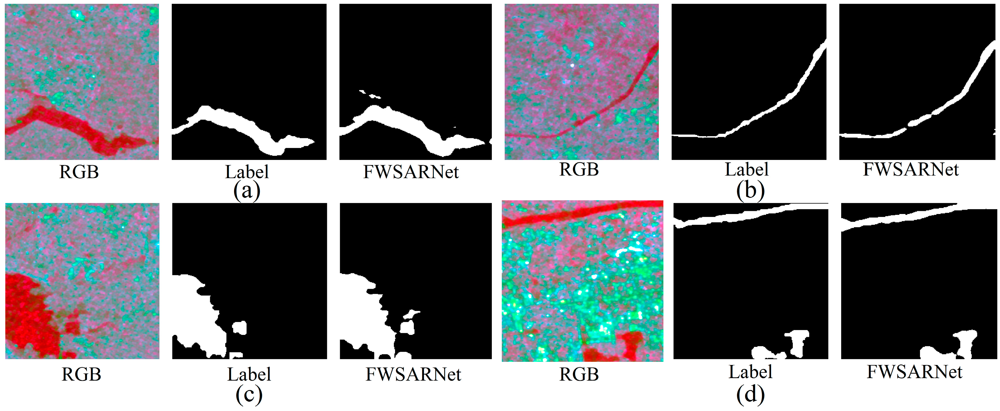
Starting from 27 July 2023, a period of prolonged heavy rainfall gripped most parts of Hebei Province, owing to the combined influence of cold and warm air masses, as well as the presence of Typhoon Doksuri. The cumulative average precipitation throughout the entire province amounted to 146.2 mm and endured for an extended duration. The continuous heavy rainfall, coupled with upstream flooding, significantly exacerbated the flood control situation in Hebei, rendering it extremely precarious. In this study, we leveraged Sentinel-1 satellite imagery acquired during the flooding and waterlogging disaster that occurred in the central region of Hebei in August 2023 to evaluate the generalization performance of the FWSARNet model. Following consistent preprocessing steps, we inputted the Sentinel-1 images from central Hebei into the FWSARNet model and compared the results with annotated images. Remarkably, the FWSARNet model demonstrated outstanding performance, yielding an F1 score of 94.03%, an Intersection over Union (IoU) of 80.79%, a mean IoU (mIoU) of 89.11%, precision at 91.25%, and a recall of 97.38%. The visualized results of the model predictions are presented in Figure 14. We have deliberately selected and showcased three typical waterbody scenarios and the results of urban flood detection. Figure 14a portrays a typical river area, while Figure 14b highlights smaller rivers and minor water bodies. Furthermore, Figure 14c provides insight into a scenario featuring a substantial water body. Upon examination of Figure 14, it becomes evident that the FWSARNet model excels not only in accurately delineating extensive water bodies but also in effectively identifying smaller rivers and tiny water bodies. The results in Figure 14d demonstrate the significant applicability of our model in urban areas. The FWSARNet model was capable of clearly distinguishing complex urban features and floods, further highlighting its robustness and generalization capability. This indicates its enormous potential in practical applications for urban flood monitoring.

5. Conclusions

This study addressed the issue of monitoring and responding to flood disasters by proposing a flood detection model, FWSARNet, based on polarized SAR data. This model utilized deformable convolution as a core operator and incorporated the structural approach of vision transformers to better capture the local details and spatial variations of flood boundaries. Additionally, it employed a multi-level feature fusion method, combining feature information from different hierarchies, enhancing the model’s expressive power and discriminative capability. In our comprehensive evaluation, we compared various backbone and decoder models. Our results clearly demonstrated that both the backbone and decoder components of the proposed model exhibited outstanding performance. FWSARNet outperformed other models in the task of SAR data flood detection and was better suited for this purpose. Furthermore, our investigation into different feature data highlights that the |VV|/|VH| ratio significantly improves the reflective properties of water bodies, thereby enhancing the performance of the flood detection model and increasing its sensitivity to changes in the water body region. To overcome the challenges posed by the scarcity of flood pixels and sample imbalance, our study conducted experiments using class weights at various ratios. Our findings reveal that the model’s optimal performance is achieved when the class weight ratio is set at 0.08:1.

6. Limitations and Prospects

Although the FWSARNet model proposed in this study had high flood detection accuracy, there are still some shortcomings. The first is image quality. The images used in this study were Sentinel-1 data, and there were fringe artifacts in the data, which may be due to sensor calibration issues or environmental interference. Although we did the filtering operation in the data pre-processing phase, we still faced some challenges. We plan to conduct in-depth research to explore ways to address these streak artifacts to further improve data quality and thus the performance of the model in real-world applications. Second, there is room for improvement in model design. Although we adopted deformable convolution v3, which is lighter than ViT and DCNv2, and reduced a large number of parameters, we recognize that there is still room for further improvement in the lightweight of the model. We plan to optimize the structure of the model at a deeper level to improve its computational efficiency and performance in real-world deployments. Third, we realize that another current limitation in the field of flood detection is the inadequacy of multi-temporal SAR images. Obtaining multi-temporal data over many years is essential to more accurately capture the dynamics of flood patterns. Therefore, future research plans include the creation of our own global multi-phase flood detection dataset to make an important contribution to flood detection research. This effort aims to fill the current gap in multi-temporal data to drive further development of flood detection technology.

Author Contributions

Methodology, H.Y. and R.W.; investigation, H.Y. and R.W.; resources, H.Y.; software, R.W.; validation, R.W.; writing—original draft preparation, R.W.; writing—review and editing, H.Y., P.L. and P.Z.; visualization, R.W. and P.L.; supervision, H.Y.; funding acquisition, H.Y. All authors have read and agreed to the published version of the manuscript.

Funding

This research was funded by the National Natural Science Foundation of China (U1304402, 41977284) and the Natural Science and Technology Project of the Natural Resources Department of Henan Province (2019-378-16).

Data Availability Statement

The ETCI_2021 Flood dataset is available online at https://www.kaggle.com/datasets/aninda/etci-2021-competition-on-flood-detection/, accessed on 17 October 2022.

Acknowledgments

The authors would like to thank the researchers who provided the open-source dataset ETCI_2021, which was very helpful to the research of this article.

Conflicts of Interest

The authors declare no conflict of interest.

References

  1. Lorenzo, A.; Berny, B.; Francesco, D.; Gustavo, N.; Ad, D.R.; Peter, S.; Klaus, W.; Luc, F. Global projections of river flood risk in a warmer world. Earth’s Future 2017, 5, 171–182. [Google Scholar]
  2. Tellman, B.; Sullivan, J.A.; Kuhn, C.; Kettner, A.J.; Doyle, C.S.; Brakenridge, G.R.; Erickson, T.A.; Slayback, D.A. Satellite imaging reveals increased proportion of population exposed to floods. Nature 2021, 596, 80–86. [Google Scholar] [CrossRef] [PubMed]
  3. Wenchao, K.; Yuming, X.; Feng, W.; Ling, W.; Hongjian, Y. Flood Detection in Gaofen-3 SAR Images via Fully Convolutional Networks. Sensors 2018, 18, 2915. [Google Scholar]
  4. Chen, Y.; Huang, J.; Song, X.; Gao, P.; Wan, S.; Shi, L.; Wang, X. Spatiotemporal Characteristics of Winter Wheat Waterlogging in the Middle and Lower Reaches of the Yangtze River, China. Adv. Meteorol. 2018, 2018, 3542103. [Google Scholar] [CrossRef]
  5. Munawar, H.S.; Hammad, A.W.A.; Waller, S.T. Remote Sensing Methods for Flood Prediction: A Review. Sensors 2022, 22, 960. [Google Scholar] [CrossRef]
  6. Kugler, Z.; De Groeve, T. The Global Flood Detection System. 2007. Available online: https://www.researchgate.net/publication/265746365_The_Global_Flood_Detection_System (accessed on 20 May 2022).
  7. Lin, Y.; Zhang, T.; Ye, Q.; Cai, J.; Wu, C.; Khirni, S.A.; Li, J. Long-term remote sensing monitoring on LUCC around Chaohu Lake with new information of algal bloom and flood submerging. Int. J. Appl. Earth Obs. Geoinf. 2021, 102, 102413. [Google Scholar] [CrossRef]
  8. Lin, L.; Di, L.; Tang, J.; Yu, E.; Zhang, C.; Rahman, M.; Shrestha, R.; Kang, L. Improvement and Validation of NASA/MODIS NRT Global Flood Mapping. Remote Sens. 2019, 11, 205. [Google Scholar] [CrossRef]
  9. Mateo, G.G.; Veitch, M.J.; Smith, L.; Oprea, S.V.; Schumann, G.; Gal, Y.; Baydin, A.G.; Backes, D. Towards global flood mapping onboard low cost satellites with machine learning. Sci. Rep. 2021, 11, 7249. [Google Scholar] [CrossRef]
  10. Tottrup, C.; Druce, D.; Meyer, R.P.; Christensen, M.; Riffler, M.; Dulleck, B.; Rastner, P.; Jupova, K.; Sokoup, T.; Haag, A.; et al. Surface Water Dynamics from Space: A Round Robin Intercomparison of Using Optical and SAR High-Resolution Satellite Observations for Regional Surface Water Detection. Remote Sens. 2022, 14, 2410. [Google Scholar] [CrossRef]
  11. Murfitt, J.; Duguay, C.R. 50 years of lake ice research from active microwave remote sensing: Progress and prospects. Remote Sens. Environ. 2021, 264, 112616. [Google Scholar] [CrossRef]
  12. Martinis, S. Automatic Near Real-Time Flood Detection in High Resolution X-Band Synthetic Aperture Radar Satellite Data Using Context-Based Classification on Irregular Graphs. Ph.D. Thesis, Faculty of Geosciences, LMU Munich, Munich, Germany, 2010. [Google Scholar]
  13. Ian, G. Polarimetric Radar Imaging: From Basics to Applications; Lee, J.-S., Pottier, E., Eds.; CRC Press: Boca Raton, FL, USA, 2012; Volume 33. [Google Scholar]
  14. Bao, L.; Lv, X.; Yao, J. Water Extraction in SAR Images Using Features Analysis and Dual-Threshold Graph Cut Model. Remote Sens. 2021, 13, 3465. [Google Scholar] [CrossRef]
  15. Shen, G.; Guo, H.; Liao, J. Object oriented method for detection of inundation extent using multi-polarized synthetic aperture radar image. J. Appl. Remote Sens. 2008, 2, 23512–23519. [Google Scholar] [CrossRef]
  16. Tong, X.; Luo, X.; Liu, S.; Xie, H.; Chao, W.; Liu, S.; Liu, S.; Makhinov, A.N.; Makhinova, A.F.; Jiang, Y. An approach for flood monitoring by the combined use of Landsat 8 optical imagery and COSMO-SkyMed radar imagery. ISPRS J. Photogramm. Remote Sens. 2018, 136, 144–153. [Google Scholar] [CrossRef]
  17. D’Addabbo, A.; Refice, A.; Pasquariello, G.; Lovergine, F.P.; Capolongo, D.; Manfreda, S. A Bayesian Network for Flood Detection Combining SAR Imagery and Ancillary Data. IEEE Trans. Geosci. Remote Sens. 2016, 54, 3612–3625. [Google Scholar] [CrossRef]
  18. Garcia-Garcia, A.; Orts-Escolano, S.; Oprea, S.; Villena-Martinez, V.; Garcia-Rodriguez, J. A Review on Deep Learning Techniques Applied to Semantic Segmentation. arXiv 2017, arXiv:1704.06857. [Google Scholar]
  19. Deng, J.; Xuan, X.; Wang, W.; Li, Z.; Yao, H.; Wang, Z. A review of research on object detection based on deep learning. J. Phys. Conf. Ser. 2020, 1684, 12028. [Google Scholar] [CrossRef]
  20. Abu, M.A.; Indra, N.H.; Rahman, A.H.A.; Sapiee, N.A.; Ahmad, I. A study on Image Classification based on Deep Learning and Tensorflow. Int. J. Eng. Res. Technol. 2019, 12, 563–569. [Google Scholar]
  21. Guo, H.; He, G.; Jiang, W.; Yin, R.; Yan, L.; Leng, W. A Multi-Scale Water Extraction Convolutional Neural Network (MWEN) Method for GaoFen-1 Remote Sensing Images. ISPRS Int. J. Geo-Inf. 2020, 9, 189. [Google Scholar] [CrossRef]
  22. Li, Z.; Liu, F.; Yang, W.; Peng, S.; Zhou, J. A Survey of Convolutional Neural Networks: Analysis, Applications, and Prospects. IEEE Trans. Neural Netw. Learn. Syst. 2022, 33, 6999–7019. [Google Scholar] [CrossRef]
  23. Long, J.; Shelhamer, E.; Darrell, T. Fully convolutional networks for semantic segmentation. In Proceedings of the 2015 IEEE Conference on Computer Vision and Pattern Recognition (CVPR), Boston, MA, USA, 7–12 June 2015; pp. 3431–3440. [Google Scholar]
  24. Olaf, R.; Philipp, F.; Thomas, B. U-Net: Convolutional Networks for Biomedical Image Segmentation. In Medical Image Computing and Computer-Assisted Intervention–MICCAI 2015: 18th International Conference, Munich, Germany, 5–9 October 2015, Proceedings, Part III 18; Springer International Publishing: New York, NY, USA, 2015. [Google Scholar]
  25. Chen, L.; Papandreou, G.; Schroff, F.; Hartwig, A. Rethinking Atrous Convolution for Semantic Image Segmentation. arXiv 2017, arXiv:1706.05587. [Google Scholar] [CrossRef]
  26. Zhou, Z.; Siddiquee, M.M.R.; Tajbakhsh, N.; Liang, J. UNet++: A Nested U-Net Architecture for Medical Image Segmentation. arXiv 2018, arXiv:1807.10165. [Google Scholar] [CrossRef]
  27. Sun, K.; Xiao, B.; Liu, D.; Wang, J. Deep High-Resolution Representation Learning for Human Pose Estimation. In Proceedings of the 2019 IEEE/CVF Conference on Computer Vision and Pattern Recognition (CVPR), Long Beach, CA, USA, 15–20 June 2019; pp. 5686–5696. [Google Scholar]
  28. Ng, K.W.; Huang, Y.F.; Koo, C.H.; Chong, K.L.; El-Shafie, A.; Najah Ahmed, A. A review of hybrid deep learning applications for streamflow forecasting. J. Hydrol. 2023, 625, 130141. [Google Scholar] [CrossRef]
  29. Essam, Y.; Huang, Y.F.; Ng, J.L.; Birima, A.H.; Ahmed, A.N.; El-Shafie, A. Predicting streamflow in Peninsular Malaysia using support vector machine and deep learning algorithms. Sci. Rep. 2022, 12, 3883. [Google Scholar] [CrossRef] [PubMed]
  30. Chen, Y.; Fan, R.; Yang, X.; Wang, J.; Latif, A. Extraction of Urban Water Bodies from High-Resolution Remote-Sensing Imagery Using Deep Learning. Water 2018, 10, 585. [Google Scholar] [CrossRef]
  31. He, Y.; Yao, S.; Yang, W.; Yan, H.; Zhang, L.; Wen, Z.; Zhang, Y.; Liu, T. An Extraction Method for Glacial Lakes Based on Landsat-8 Imagery Using an Improved U-Net Network. IEEE J. Sel. Top. Appl. Earth Observ. Remote Sens. 2021, 14, 6544–6558. [Google Scholar] [CrossRef]
  32. Zhong, H.; Sun, H.; Han, D.; Li, Z.; Jia, R. Lake water body extraction of optical remote sensing images based on semantic segmentation. Appl. Intell. 2022, 52, 17974–17989. [Google Scholar] [CrossRef]
  33. Wang, Z.; Gao, X.; Zhang, Y.; Zhao, G. MSLWENet: A Novel Deep Learning Network for Lake Water Body Extraction of Google Remote Sensing Images. Remote Sens. 2020, 12, 4140. [Google Scholar] [CrossRef]
  34. Edoardo, N.; Joseph, B.; Samir, B.; Lars, B. Fully Convolutional Neural Network for Rapid Flood Segmentation in Synthetic Aperture Radar Imagery. Remote Sens. 2020, 12, 2532. [Google Scholar]
  35. Peng, B.; Huang, Q.; Vongkusolkit, J.; Gao, S.; Wright, D.B.; Fang, Z.N.; Qiang, Y. Urban Flood Mapping With Bitemporal Multispectral Imagery Via a Self-Supervised Learning Framework. Ieee J. Sel. Top. Appl. Earth Observ. Remote Sens. 2021, 14, 2001–2016. [Google Scholar] [CrossRef]
  36. Yuan, K.; Zhuang, X.; Schaefer, G.; Feng, J.; Guan, L.; Fang, H. Deep-Learning-Based Multispectral Satellite Image Segmentation for Water Body Detection. IEEE J. Sel. Top. Appl. Earth Observ. Remote Sens. 2021, 14, 7422–7434. [Google Scholar] [CrossRef]
  37. Vaswani, A.; Shazeer, N.; Parmar, N.; Uszkoreit, J.; Jones, L.; Gomez, A.N.; Kaiser, Ł. Attention Is All You Need. 2017. Available online: https://proceedings.neurips.cc/paper_files/paper/2017/hash/3f5ee243547dee91fbd053c1c4a845aa-Abstract.html (accessed on 16 July 2023).
  38. Dosovitskiy, A.; Beyer, L.; Kolesnikov, A.; Weissenborn, D.; Zhai, X.; Unterthiner, T.; Dehghani, M.; Minderer, M.; Heigold, G.; Gelly, S.; et al. An Image is Worth 16 × 16 Words: Transformers for Image Recognition at Scale. arXiv 2021, arXiv:2010.11929. [Google Scholar]
  39. Abed, M.; Imteaz, M.A.; Ahmed, A.N.; Huang, Y.F. A novel application of transformer neural network (TNN) for estimating pan evaporation rate. Appl. Water Sci. 2023, 13, 31. [Google Scholar] [CrossRef]
  40. Ma, D.; Jiang, L.; Li, J.; Shi, Y. Water index and Swin Transformer Ensemble (WISTE) for water body extraction from multispectral remote sensing images. Giscience Remote Sens. 2023, 60, 2251704. [Google Scholar] [CrossRef]
  41. He, K.; Zhang, X.; Ren, S.; Sun, J. Deep Residual Learning for Image Recognition. In Proceedings of the 2016 IEEE Conference on Computer Vision and Pattern Recognition (CVPR), Las Vegas, NV, USA, 27–30 June 2016; pp. 770–778. [Google Scholar]
  42. Ding, X.; Zhang, X.; Zhou, Y.; Han, J.; Ding, G.; Sun, J. Scaling Up Your Kernels to 31 × 31: Revisiting Large Kernel Design in CNNs. arXiv 2022, arXiv:2203.06717. [Google Scholar]
  43. Chen, F.; Wu, F.; Xu, J.; Gao, G.; Ge, Q.; Jing, X. Adaptive deformable convolutional network. Neurocomputing 2021, 453, 853–864. [Google Scholar] [CrossRef]
  44. Wang, W.; Dai, J.; Chen, Z.; Huang, Z.; Li, Z.; Zhu, X.; Hu, X.; Lu, T.; Lu, L.; Li, H.; et al. InternImage: Exploring Large-Scale Vision Foundation Models with Deformable Convolutions. arXiv 2023, arXiv:2211.05778. [Google Scholar]
  45. Zhao, H.; Shi, J.; Qi, X.; Wang, X.; Jia, J. Pyramid Scene Parsing Network. arXiv 2017, arXiv:1612.01105. [Google Scholar]
  46. Aldahoul, N.; Momo, M.A.; Chong, K.L.; Ahmed, A.N.; Huang, Y.F.; Sherif, M.; El-Shafie, A. Streamflow classification by employing various machine learning models for peninsular Malaysia. Sci. Rep. 2023, 13, 14574. [Google Scholar] [CrossRef]
  47. Woodworth, B.; Patel, K.K.; Stich, S.U.; Dai, Z.; Bullins, B.; Mcmahan, H.B.; Shamir, O.; Srebro, N. Is Local SGD Better than Minibatch SGD? arXiv 2020, arXiv:2002.07839. [Google Scholar]
  48. Kingma, D.P.; Ba, J. Adam: A Method for Stochastic Optimization. arXiv 2017, arXiv:1412.6980. [Google Scholar]
  49. Loshchilov, I.; Hutter, F. Decoupled Weight Decay Regularization. arXiv 2019, arXiv:1711.05101. [Google Scholar]
  50. Llugsi, R.; Yacoubi, S.E.; Fontaine, A.; Lupera, P. Comparison between Adam, AdaMax and Adam W optimizers to implement a Weather Forecast based on Neural Networks for the Andean city of Quito. In Proceedings of the 2021 IEEE Fifth Ecuador Technical Chapters Meeting (ETCM), Cuenca, Ecuador, 12–15 October 2021; pp. 1–6. [Google Scholar]
  51. Chu, X.; Tian, Z.; Wang, Y.; Zhang, B.; Ren, H.; Wei, X.; Xia, H.; Shen, C. Twins: Revisiting the Design of Spatial Attention in Vision Transformers. arXiv 2021, arXiv:2104.13840. [Google Scholar]
  52. Liu, Z.; Lin, Y.; Cao, Y.; Hu, H.; Wei, Y.; Zhang, Z.; Lin, S.; Guo, B. Swin Transformer: Hierarchical Vision Transformer using Shifted Windows. arXiv 2021, arXiv:2103.14030. [Google Scholar]
  53. Chen, L.; Papandreou, G.; Kokkinos, I.; Murphy, K.; Yuille, A.L. DeepLab: Semantic Image Segmentation with Deep Convolutional Nets, Atrous Convolution, and Fully Connected CRFs. IEEE Trans. Pattern Anal. Mach. Intell. 2018, 40, 834–848. [Google Scholar] [CrossRef] [PubMed]
  54. Tsung-Yi, L.; Dollár, P.; Girshick, R.; He, K.; Hariharan, B.; Belongie, S. Feature Pyramid Networks for Object Detection. arXiv 2017, arXiv:1612.03144. [Google Scholar]
  55. Xie, E.; Wang, W.; Yu, Z.; Anandkumar, A.; Alvarez, J.M.; Luo, P. SegFormer: Simple and Efficient Design for Semantic Segmentation with Transformers. arXiv 2021, arXiv:2105.15203. [Google Scholar]
  56. Sayak, P.; Ganju, S. Flood Segmentation on Sentinel-1 SAR Imagery with Semi-Supervised Learning. arXiv 2021, arXiv:2107.08369. [Google Scholar]
  57. Ghosh, B.; Garg, S.; Motagh, M. Automatic Flood Detection from Sentinel-1 Data Using Deep Learning Architectures. ISPRS Ann. Photogramm. Remote Sens. Spat. Inf. Sci. 2022, V-3-2022, 201–208. [Google Scholar] [CrossRef]
  58. Garg, S.; Ghosh, B.; Motagh, M. Automatic Flood Detection from Sentinel-1 Data Using Deep Learning: Demonstration of NASA-ETCI Benchmark Datasets. 2022. Available online: https://ui.adsabs.harvard.edu/abs/2021AGUFM.H55A0739G/abstract (accessed on 16 July 2023).
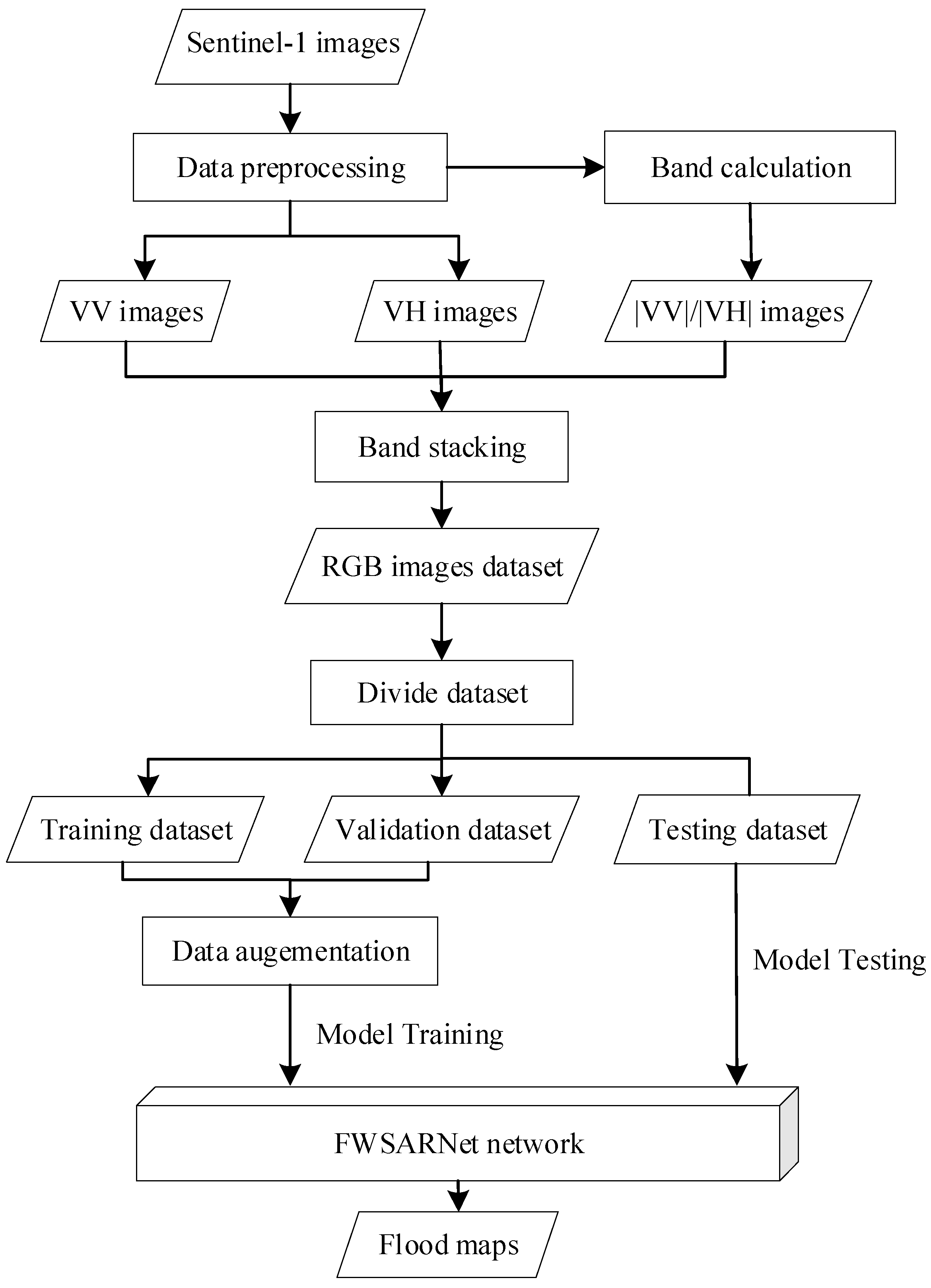
Figure 1. The flowchart of this study.
Water 15 04202 g001
Figure 2. The structure of the FWSARNet.
Water 15 04202 g002
Figure 3. The structure of the Stem Layer.
Water 15 04202 g003
Figure 4. The structure of the Feature Extraction Module.
Water 15 04202 g004
Figure 5. The structure of Deformable Convolution v3.
Water 15 04202 g005
Figure 6. The structure of the Pyramid pool module.
Water 15 04202 g006
Figure 7. The structure of the Fusion Module.
Water 15 04202 g007
Figure 8. Raw data (VV and VH tiles), RGB data for training, Water Body/Land Image, Flood Image, and Label for training.
Water 15 04202 g008
Figure 9. The training loss curves and resulting curves of the evaluation metrics. (a) loss curves; (b) resulting curves of the evaluation metrics.
Water 15 04202 g009
Figure 10. (a) Loss values using different optimizers; (b) IoU of floods using different optimizers; (c) Precision using different optimizers; (d) Recall using different optimizers.
Water 15 04202 g010
Figure 11. The extract results of different backbones in the testing region. The red box highlights areas of contrast.
Water 15 04202 g011
Figure 12. The extract results of different decode_head in the testing region. The red box highlights areas of contrast.
Water 15 04202 g012
Figure 13. (a) Number of Anchors for Flood and Background; (b) Comparison results of different Class weight ratios.
Water 15 04202 g013
Figure 14. The results of the generalization experiment of the FWSARNet model on flood disaster in central Hebei Province. (a) The prediction results for typical rivers; (b) The prediction results for tiny rivers; (c) The prediction results for widespread flooding; (d) Prediction results for flooding in urban areas.
Water 15 04202 g014
Table 1. Comparison of experimental results of different backbones.
BackboneIou (%)mIou (%)F1 (%)Precision (%)Recall (%)
ViT68.2181.4489.1891.4287.26
ResNet76.2186.1792.2694.2590.51
Swin Transformer77.0886.6892.5894.5990.81
Twins_svt77.8087.1392.8695.3890.69
FWSARNet80.1088.4793.6794.8492.59
Table 2. Comparison of experimental results of different decoders.
DecoderIou (%)mIou (%)F1 (%)Precision (%)Recall (%)
ASPP71.3983.2590.490.5390.28
DSASPP77.5287.0792.8196.5489.81
FPN77.9987.392.9695.8490.53
Segformer79.3288.0793.4295.9591.25
FWSARNet80.188.4793.6794.8492.59
Table 3. Comparison of the computational efficiency of different models.
ModelFlops (G)Params (M)Test Time (s)Train Time (min)
ViT98.51144.06267409.96
ResNet99.1766.4182318.07
Swin Transformer66.3981.15225272.27
Twins_svt63.3387.61232286.22
FWSARNet58.7558.96140263.23
Table 4. Accuracy comparison of different features in the testing region.
DATAVVVH|VV|/|VH|IoU (%)
ETCI2021+76.18
+78.14
++78.25
+++80.1
Note: where “+” means the feature is introduced and “−” means the feature is not introduced.
Disclaimer/Publisher’s Note: The statements, opinions and data contained in all publications are solely those of the individual author(s) and contributor(s) and not of MDPI and/or the editor(s). MDPI and/or the editor(s) disclaim responsibility for any injury to people or property resulting from any ideas, methods, instructions or products referred to in the content.