Flood Estimation and Control in a Micro-Watershed Using GIS-Based Integrated Approach

Abstract

Flood analyses when using a GIS-based integrated approach have been successfully applied around the world in large-sized watersheds. This study employed hydrological-hydraulic modeling to analyze flash floods by integrating HEC-HMS, HEC-RAS, and ArcGIS software for flood evaluation and control in a micro-watershed in the Samaru River, Nigeria. The watershed boundaries, its characteristics (soil and land use), the topographical survey, and the intensity duration frequency curve (IDF) of the study area were produced using data-driven techniques. The HEC-HMS model was used to derive the peak discharges for 2-, 5-, 10-, 25-, 50-, 100-, and 200-year return periods with the frequency storm method. Afterward, the water surface profiles for the respective return periods were estimated using the HEC-RAS hydrodynamic model. The simulated design flood for the 2-, 5-, 10-, 25-, 50-, 100-, and 200-year return periods at the reference location (the NUGA gate culvert) were 3.5, 6.8, 9.1, 12.1, 14.3, 16.6, and 19.0 m³/s, respectively, while those at the watershed outlet for the respective return periods were 7.5, 14.9, 20.3, 27.3, 32.6, 38.0, and 43.5 m³/s, respectively (with a water height of 0.9 m, 1.1 m, 1.3 m, 1.33 m, 1.38 m, 1.5 3m, and 1.8 m, respectively), at the NUGA gate culvert cross-section. The maximum water depths of about 0.9 m and 1.0 m were recorded in the right and left overbanks, which were similar to the simulated water depth for the 2- and 5-year return periods. Hence, for the smart control of floods passing through the river and major hydraulic structures, a minimum design height of 1.50 m is recommended. For the most economic trapezoidal channel section, a normal depth of 1.50 m, a bottom width of 1.73 m, a top width of 3.50 m, and a free board of 0.30 m is proposed to curb the overtopping of floods along the channel sub-sections. The findings of this study could help hydraulic engineers minimize flooding in streams and rivers overbanks in a micro-watershed.

1. Introduction

As a result of climate change, flooding is an increasing natural disaster that is bedeviling every nation worldwide. It causes catastrophic damage to ecosystems, life losses, and economic losses [1,2,3,4,5,6,7,8]. In Nigeria, flooding effects are similar to those in the rest of the world [6,9,10,11,12,13,14]. According to Cirella and Iyalomhe, [15] flooding displaces more people than any other disaster in Nigeria because about 20% of the population are at risk of flooding. Recently, floods have displaced about 2.3 million people, and this has resulted in the unfortunate loss of 363 lives. Additionally, approximately 16 million individuals were affected in various ways, thus leading to severe economic losses. Consequently, a state of emergency was recently declared in nine states of the nation by the Nigerian government [10,11,13,16].

Storm water flows through an open channel with high velocity as runoff; this flow may be unsteady, non-uniform, or backflow-dependent upon the channel geometry, obstructions in the channel, catchment characteristics, and the amount of runoff from the catchment. High floods tends to erode channel bottoms, which may lead to channel bank collapse, as well as to modifications to the channel geometry [17,18,19]. This usually results in spilling out of a reasonable quantity of water from the channel [18,20]. It is not possible for a natural or artificial waterway to remain unchanged during the urban development process because land use changes have a great influence on runoff generation [18,21,22]. Residential and industrial development have been the main activities taking place in micro-watersheds. In most cases, the stormwater from an upper catchment is conveyed through an unlined natural open channel to the watershed outlets. Thus, some sections of these channels collapse, and several diversion channels are formed by the flowing water; as such, a reasonable quantity of water can be lost via these channels, and this can be coupled with evaporation and infiltration losses. It is anticipated that these losses could be so high as to result in inadequate discharges, which are unable to reach the outlet. Moreover, a flow conveyance structure along the channel is normally constructed to allow access, but it might be in danger of washing away or collapsing as water overflows its top when there is excess rainfall. Having said this, owing to the above concerns, it has become imperative to model the flow and optimize channel geometry in order to design preventive and control measures through which to limit water loss and the collapse of conveyance structures. This can only be achieved by carrying out detailed hydrologic and hydraulic modeling.

Floodplain mapping has, in the past, been carried out using conventional methods [23,24]. These methods are tedious, time-consuming, and relatively expensive. In addition, they require considerable fieldwork and the maintenance of long-term river and stream records, which are not readily available for catchments (which are mostly ungauged) in a large developing country such as Nigeria [9,25,26]. These challenges could be addressed using an integrated approach of hydrologic and hydrodynamic modeling along with Arc-GIS analysis, which is less tedious and faster, more effective, and reliable, and it makes the immediate assessment of natural resources possible and more accurate [9,21,27]. Hydrological modeling aids in determining the catchment response to rainfall events [21]. Floodplain modeling is mainly concerned with the hydrological behavior of watersheds for a particular rainfall event. The development of flood management strategies and flood damage reduction and mitigation for an ungauged catchment has remained a big challenge to engineers and policymakers [6,28]. This is genuinely true because detailed hydrological modeling is highly necessary for the estimation of flood volume and its recurrence time, which are the key parameters on which floods solutions are based [29]. Hydraulic modeling results help to provide a set of actions and preventive measures that can be undertaken to curtail flood occurrences and flood aftermaths [30,31,32,33].

In this study, the Hydrologic Engineering Center-Hydrological Model System (HEC-HMS) and the Hydrologic Engineering Center-River Analysis System (HEC-RAS) were coupled alongside Arc-GIS to perform hydrologic and hydrodynamic modeling in a micro-watershed. These packages were produced by the Hydrologic Engineering Center (HEC) of the US Army Corps of Engineers. The latter was used for simulating rainfall runoff, and it has the capability of modeling a wide range of geographic expanses, including flood hydrology [18,21,34]. The former was used for the simulation of design floods and water surface profiles, which relies on I-D energy equation results [35,36]. Abdessamed and Abderrazak, [37] who coupled their work with HEC-RAS and HEC-HMS, performed rainfall runoff modeling for floodplain inundation mapping in a data-sparse environment. Laouacheria and Mansouri [38] employed the frequency storm approach in the HEC-HMS model to simulate runoff in a small urban catchment in the northeast region of Algeria. An integrated hydrologic and hydraulic modeling was performed for a medium-sized, ungagged urban watershed using HEC-HMS and HEC-RAS by Natarajan and Radhakrishnan [35]. Bruno et al. [39] applied hydrological and hydraulic modeling via integrating HEC-HMS and HEC-RAS, and they analyzed flash flood events in a small urban stream.

In this study, we conducted a comprehensive analysis of a data-sparse micro-watershed in Nigeria by employing a coupled hydrological-hydraulic modeling methodology that uses HEC-HMS and HEC-RAS. The goal was to provide a framework for other researchers to assess and validate their own flash flood modeling methodologies within a similar micro-watershed context. The study analyzed flood frequencies, peak discharges, and their effects on the flood frequencies. The specific objective of the study was to determine water surface profiles for different return periods and to propose smart flood control structures that will safely convey the excess floods to the watershed outlet. It is hoped that the information from this study will help inform the policy and decision makers within relevant authorities to be aware of flood-prone areas along streams, which will, in turn, help in planning for future flooding events.

2. Materials and Methods

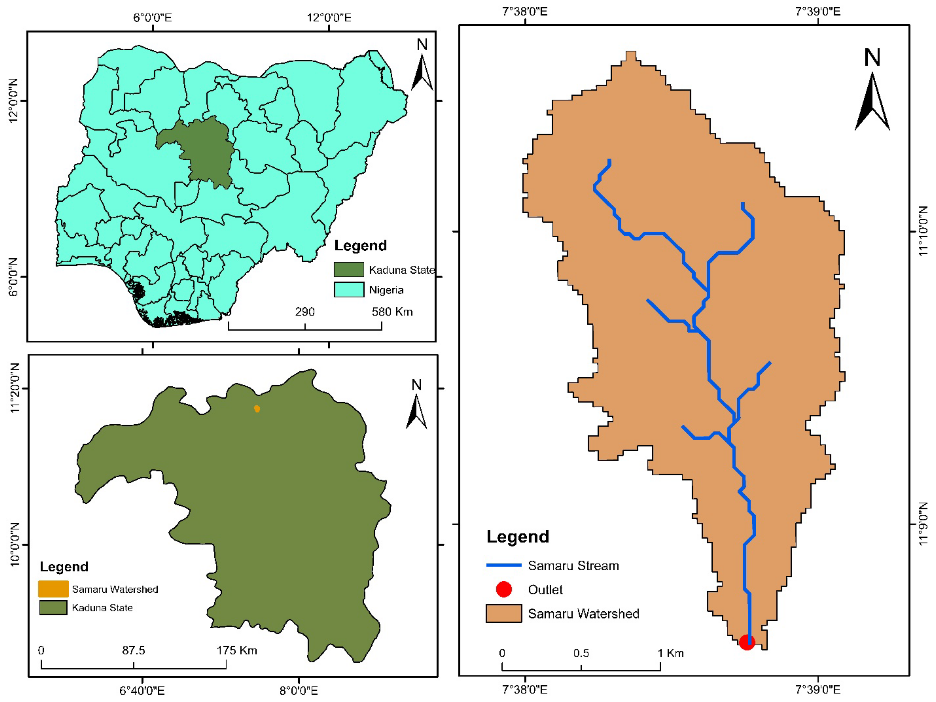
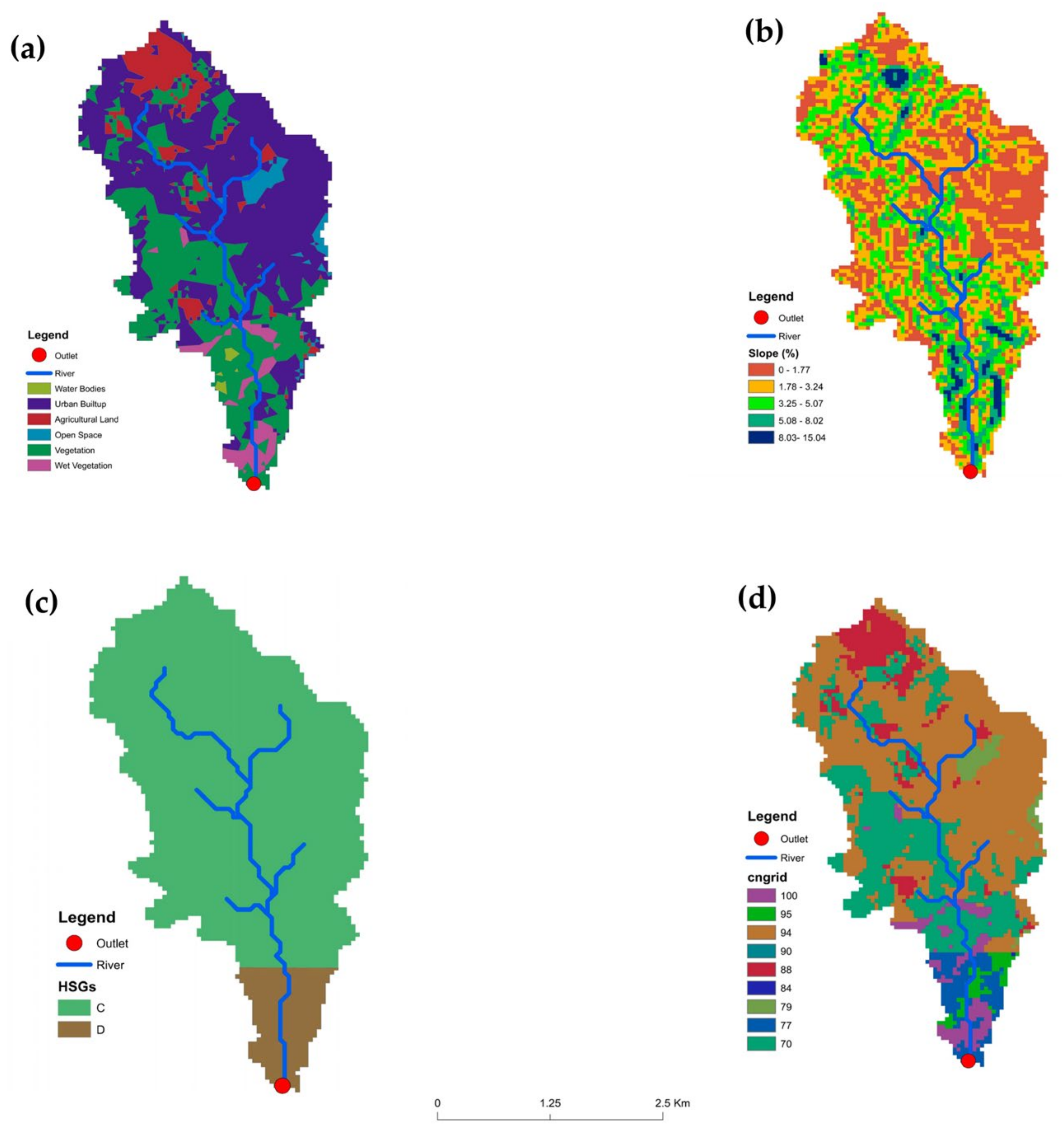
2.1. Study Area and Data Collection

The study area is within Zaria, Kaduna State, Nigeria. Zaria is one of the provinces that makes up the Central High Plains of Northern Nigeria, and it is approximately 670 m above mean sea level (Figure 1). It is located about 950 km away from Lagos; it covers a total landmass of about 61 km², thus making it a nodal point in terms of road and rail transport because of its locational factors [40,41].

The sub-catchment is a 1st-order minor tributary of the Kubanni River within the Kubanni drainage basin, lying between 110°08′32″ and 110°09′38″ N, and 70°38′36″ and 70°38′48″ E. The stream has a length of 1.05 km, a basin area of 2.28 km², a drainage density of 0.4605 m/km², and a relative relief of 30.48 m. It has a maximum depth of 3.01 m and a maximum width of 10.8 m [40,41]. This stream flows in the southeast direction of Samaru through Ganga Uku and Ahmadu Bello University, Zaria to the Kubanni reservoir. For the land use characteristics of the watershed (Figure 2a), it has six main classes, which are as follows: urban build up (57.5%), open space (4.2%), agricultural land (8.1%), vegetation (26.2%), wet vegetation (3%), and Water bodies (1%). The highest elevation in the watershed is 716 m, while the lowest elevation is 640 m. Also, the catchment is very sloped at the downstream part of the Samaru River, as shown in Figure 2b. The mean slope of the watershed is 2.8%, while the maximum and minimum slopes are 15% and 0%, respectively. Analysis of the soil hydrologic characteristics shows that the dominant hydrological soil group is C, which covers 3.76 km² (90.4%) of the watershed and is at the upstream part (Figure 2c); meanwhile, group D covers 0.39 km² (9.6%) at the far downstream near the outlet. The curve number (CN) grid of the watershed shows (Figure 2d) that the maximum curve number is 100 while the minimum is 70, and the mean curve number in the watershed is 86.2.

The data used in this study and their sources are summarized in

Table 1. Data type and sources of the data.

S/N	Data Category	Data Type	Data Source
1	Satellite imagery (Landsat 8 OLI)	Land use data (30 m)	United State Geological Survey (USGS)
2	GIS data	SRTM DEM (30 m)	United State Geological Survey (USGS)
		Slope
3	Meteorological data	Rainfall data	Nigerian Meteorological Agency (NiMet)
		Observed discharge data	[41]
4	Geomorphological data	Soil data (10 m)	Digital World Soil Map (FAO)
5	Ancillary data	Channel cross-section and elevation data	Field (Topographical survey)

. The channel cross-section data was obtained through a topographical survey that was constructed using Total Station (Tables S1 and S2). Climate and geospatial data were utilized to drive the HEC-HMS and HEC-RAS models. The Landsat 8 Operational Land Imager (OLI) with spatial resolution of 30 m, wasobtained from the United States Geological Survey (USGS) Global Visualization Viewer GLOVIS. The land use classification was achieved using the supervised classification method, and it was evaluated using onsite data. The accuracy of the LULC map was assessed using ground truthing and by comparing the data from the field. A confusion matrix was constructed to estimate the producer, user, and kappa accuracy (with a kappa index of 96%). The Shuttle Radar Topography Mission (SRTM) DEM data with a spatial resolution of 30 m were downloaded from GLOVIS, and the source of the data for the soil map was the Food and Agricultural Organization (FOA). A time series of the climate data (rainfall data from the Nigerian College of Aviation Technology, Zaria station) was obtained from the Nigerian Meteorological Agency (NiMet), which covered the period from 1967 to 2017 (i.e., 50 years of data).

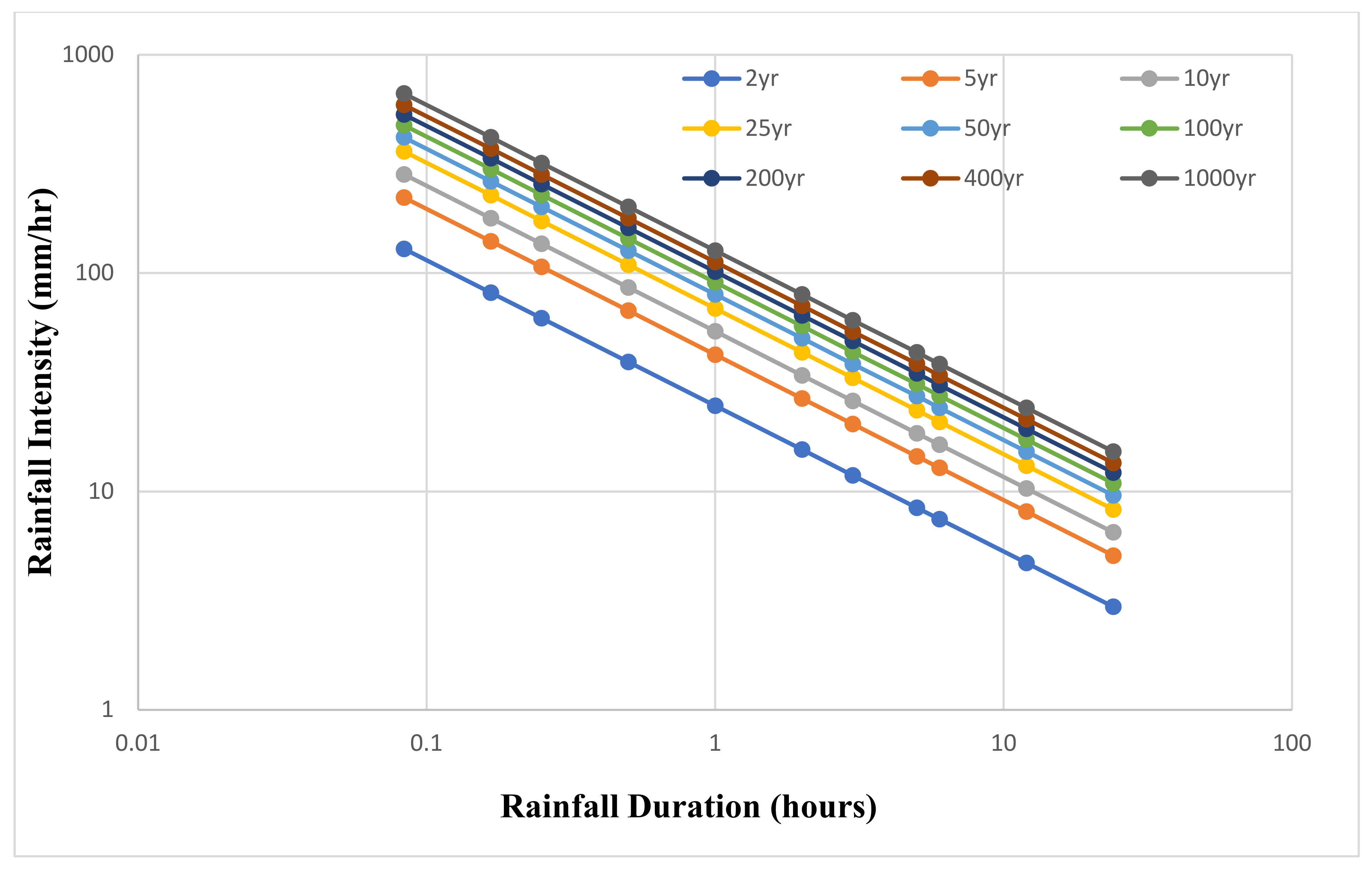
2.2. Intensity Duration Frequency Curve IDF

Intensity duration frequency curve (IDF) development is the first step for HEC-HMS hydrologic simulation when using the frequency storm method. The peak discharges (Qmax) were determined for different return periods. The maximum daily (24 h) precipitation data for 1968–2017 in Samaru was reduced to a shorter time scale of 10, 20, 30, 60, 120, 360, 720, and 1440 min using the formula recommended by the Indian Meteorological Department [42,43]. The formula has been widely used and has gained acceptance worldwide [44,45,46,47,48].

The required precipitation depth of less than 24 h is given by Equation (1).

$${\mathit{P}}_{\mathit{t}}={\mathit{P}}_{24}{\left[\frac{\mathit{t}}{24}\right]}^{\left(\frac{1}{3}\right)},$$

(1)

where ${\mathit{P}}_{\mathit{t}}=$ the required precipitation depth for a duration less than 24 h in mm, ${\mathit{P}}_{24}=$ the daily precipitation depth in mm, and $\mathit{t}=$ the required time duration in hours.

To determine the intensity, duration, and frequency curves of the Samaru stream watershed, vital input data for the HEC-HMS simulation and Gumbel’s statistical distribution for frequency analysis were utilized. This method is often used to predict extreme hydrological events such as floods [49,50]. The cumulative distribution function (cdf) of the Gumbel extreme value distribution (maximum) is given by the following [50]:

$$\mathit{F}(\mathit{X})=\mathit{exp}\left[-\mathit{exp}(-\mathit{y})\right]={\mathit{e}}^{-{\mathit{e}}^{-\mathit{y}}},$$

(2)

where $\mathit{F}\left(\mathit{X}\right)=$ the probability distribution function of a random variable $\mathit{x}$, and $\mathit{y}=$ the reduced variate.

The probability of exceedance is related to the return period $\left(\mathit{T}\right)$. The probability of exceedance of the excluded events is thus

$${\mathit{F}}_1(\mathit{X})=1-\mathit{F}(\mathit{X})=\frac{1}{\mathit{T}},$$

(3)

where ${\mathit{F}}_1\left(\mathit{X}\right)=$ the probability of exceedance at a return period $\left(\mathit{T}\right)$, and $\mathit{T}$ = the return period.

Combining Equations (2) and (3) yields

$$\frac{1}{\mathit{T}}=1-{\mathit{e}}^{-{\mathit{e}}^{-\mathit{y}}},$$

(4)

where $\mathit{T}$ = the return period, and $\mathit{y}=$ the reduced variate.

The reduced variate from Equation (4) may be transformed into the following form

$$\mathit{y}=-\mathit{I}\mathit{n}\left\{\mathit{I}\mathit{n}\left[\frac{\mathit{T}}{\left(\mathit{T}-1\right)}\right]\right\}.$$

(5)

The Gumbel’s reduced variate is represented by a linear relationship with Gumbel’s reduced mean variable ${\overline{\mathit{y}}}_{\mathit{n}}$, standard deviation ${\mathit{\sigma }}_{\mathit{n}}$, and frequency factor $\mathit{K}$. Thus, we have

$$\mathit{y}={\overline{\mathit{y}}}_{\mathit{n}}+\mathit{K}.{\mathit{\sigma }}_{\mathit{n}}.$$

(6)

Hence, $\mathit{K}$ is then

$$\mathit{K}=\frac{\mathit{y}-{\overline{\mathit{y}}}_{\mathit{n}}}{{\mathit{\sigma }}_{\mathit{n}}}=\frac{\left(-\mathit{I}\mathit{n}\left\{\mathit{I}\mathit{n}\left[\frac{\mathit{T}}{\mathit{T}-1}\right]\right\}\right)-{\overline{\mathit{y}}}_{\mathit{n}}}{{\mathit{\sigma }}_{\mathit{n}}}.$$

(7)

The frequency factor $\mathit{K}$ for a Gumbel distribution is also given by Equation (8)

$$\mathit{K}=\frac{\sqrt{6}}{\mathit{\pi }}\left\{0.5772+\mathit{I}\mathit{n}\left[\mathit{I}\mathit{n}\left(\frac{\mathit{T}}{\mathit{T}-1}\right)\right]\right\},$$

(8)

where $\mathit{T}$ = the return periods, and $\mathit{K}=$ the frequency factor.

The Gumbel equation for the total maximum precipitation for a given return period is given as

$${\mathit{P}}_{\mathit{T}}=\overline{\mathit{P}}+\mathit{K}{\mathit{\sigma }}_{\mathit{x}},$$

(9)

where ${\mathit{P}}_{\mathit{T}}=$ the magnitude of precipitation for a $\mathit{T}$ return period, $\overline{\mathit{P}}=$ the mean maximum precipitation for $\mathit{n}$ years, and ${\mathit{\sigma }}_{\mathit{x}}=$ the standard deviation of the sample size.

The mean maximum precipitation for $\mathit{n}$ years $\overline{\mathit{P}}$ is given by the expression below:

$$\overline{\mathit{P}}=\frac{{\sum }_{\mathit{i}=1}^{\mathit{n}}{\mathit{P}}_{\mathit{i}}}{\mathit{n}},$$

(10)

where $\overline{\mathit{P}}=$ the mean maximum precipitation for $\mathit{n}$ years, ${\mathit{P}}_{\mathit{i}}=$ the maximum precipitation of the $\mathit{i}\mathit{t}\mathit{h}$ year, $\mathit{n}$ = the number of sample size/number of years of record.

The standard deviation of the sample size ${\mathit{\sigma }}_{\mathit{x}}$ is given by Equation (11)

$${\mathit{\sigma }}_{\mathit{x}}=\sqrt{\frac{1}{\left(\mathit{n}-1\right)}{\sum }_{\mathit{i}=1}^{\mathit{n}}{\left({\mathit{P}}_{\mathit{i}}-\overline{\mathit{P}}\right)}^2},$$

(11)

where ${\mathit{\sigma }}_{\mathit{x}}=$ the standard deviation of the sample size, $\overline{\mathit{P}}=$ the mean maximum precipitation for $\mathit{n}$ years, ${\mathit{P}}_{\mathit{i}}=$ the maximum precipitation of the $\mathit{i}\mathit{t}\mathit{h}$ year, and $\mathit{n}$ = the sample size/number of years of record.

The intensity of precipitation (mm/h) for any time duration $\mathit{t}$ for all the respective return periods was calculated using Equation (12)

$$\mathit{I}=\frac{{\mathit{P}}_{\mathit{T}}}{\mathit{t}},$$

(12)

where $\mathit{I}=$ the intensity of rainfall in mm/h, ${\mathit{P}}_{\mathit{T}}=$ the precipitation depth in mm, and $\mathit{t}=$ the time duration of rainfall in hours.

For the estimation of the maximum precipitation when using the Gumbel distribution in this study, 50 years of maximum annual precipitation data of the Samaru stream watershed from 1968 to 2017 were considered.

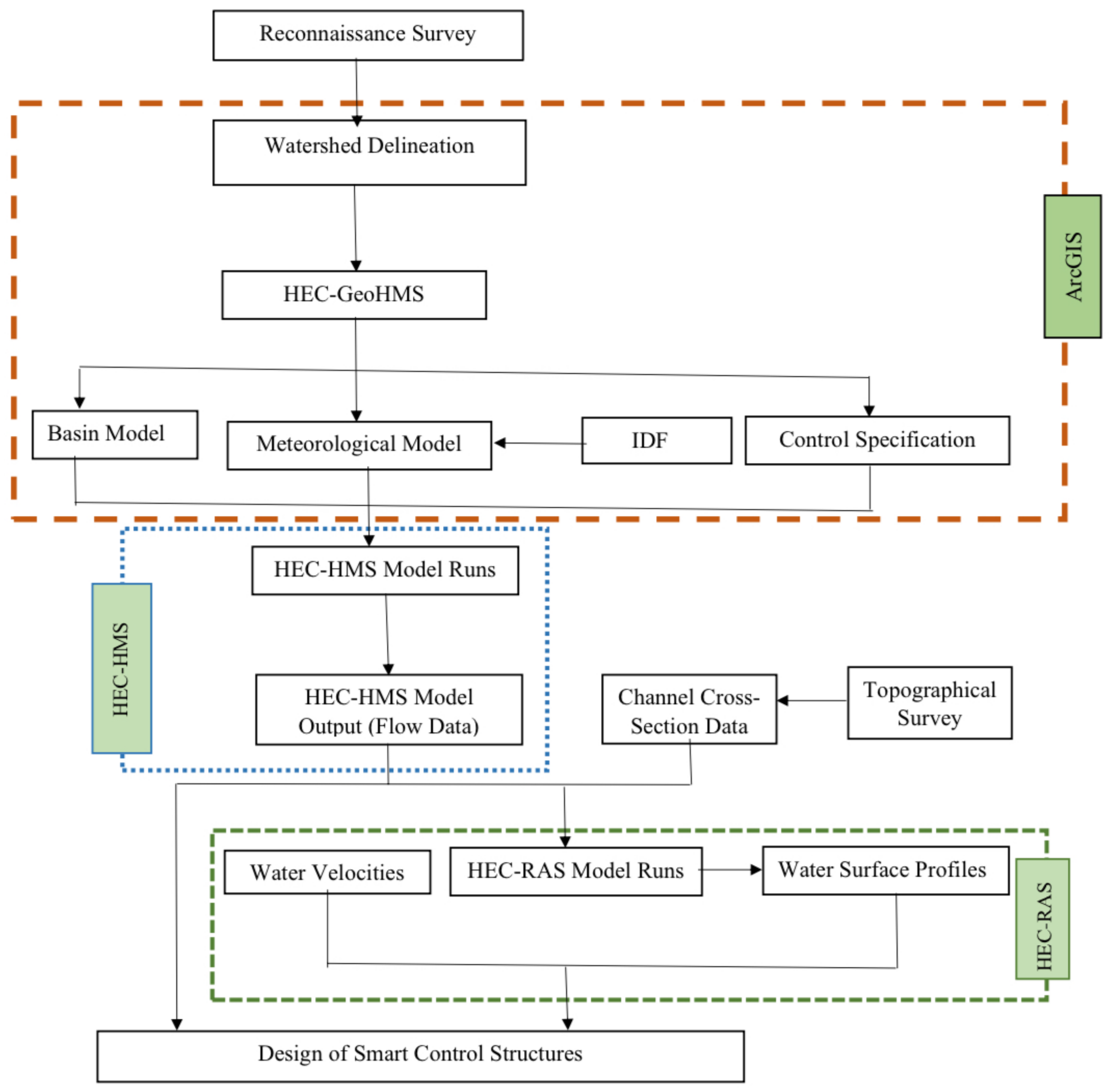
2.3. Model Setup and Evaluation

The methodological sequence of the model connections, evaluation, and development used in this study, from the onset to completion, is presented in Figure 3.

2.3.1. HEC-HMS Model

The HEC-HMS basin model contains information relevant to the physical attributes of a watershed, such as the basin area, river reach connectivity, or reservoir data. The model of the Samaru basin contains four of these elements, and they were developed in Arc-GIS using the HEC-GeoHMS extension. A total of 18 hydrologic elements were generated for the Samaru model, which consists of 9 sub-basins, 4 river reaches, 4 junctions, and 1 outlet (at the point where the Samaru stream drains into the Malmo River). Although, the meteorologic model was developed based on the climatic data of the study area, afterward, the control specifications were defined. In this study, hourly time intervals were used and simulated for only two days. This period was selected based on the temporal size of the observed streamflow. The HEC-HMS model for the Samaru watershed was calibrated and validated with the August and September 2014 daily discharge data, which were obtained from a gauge station located at the outlet of the watershed. The choice of the August and September data was made because we are interested in peak discharge, and in those periods of the year the watershed usually experiences flood events. An auto-optimization operation and the peak weighted root mean square error (PWRMSE) were selected as objective functions in the HEC-HMS model during the calibration of the model parameters. This approach was selected because of its simplicity and high performance [21,37,51]. A sensitivity analysis of the model parameter was performed by varying the values of the respective model parameters by ±20% at 5% intervals. The parameters checked were the curve number, lag time, percentage imperviousness, and Muskingum K. The percentage change in the simulated peak flow and volume as a result of variations in the respective model parameters was plotted. The model’s performance was evaluated using statistical hydrologic indices of the agreement between the observed and simulated runoff values. The indices used were the root mean square error (RMSE), the Nash–Sutcliffe efficiency (NSE), and percentage bias (PBIAS).

$$\mathit{R}\mathit{M}\mathit{S}\mathit{E}=\sqrt{\frac{1}{\mathit{N}}{\sum }_{\mathit{i}=1}^{\mathit{n}}{\left({\mathit{Q}}_{\mathit{o}\mathit{b}\mathit{s}}-{\mathit{Q}}_{\mathit{c}\mathit{o}\mathit{m}\mathit{p}}\right)}_{\mathit{i}}^2}$$

(13)

$$\mathit{N}\mathit{S}\mathit{E}=100\left[1-\frac{{\sum }_{\mathit{i}=1}^{\mathit{n}}{\left({\mathit{Q}}_{\mathit{o}\mathit{b}\mathit{s}}-{\mathit{Q}}_{\mathit{c}\mathit{o}\mathit{m}\mathit{p}}\right)}_{\mathit{i}}^2}{{\sum }_{\mathit{i}=1}^{\mathit{n}}{\left({\mathit{Q}}_{\mathit{o}\mathit{b}\mathit{s}}-\overline{{\mathit{Q}}_{\mathit{o}\mathit{b}\mathit{s}}}\right)}_{\mathit{i}}^2}\right]$$

(14)

$$\mathit{P}\mathit{B}\mathit{I}\mathit{A}\mathit{S}=100\left[\frac{{\sum }_{\mathit{i}=1}^{\mathit{n}}\left({\mathit{Q}}_{\mathit{o}\mathit{b}\mathit{s}}-{\mathit{Q}}_{\mathit{c}\mathit{o}\mathit{m}\mathit{p}}\right)}{{\sum }_{\mathit{i}=1}^{\mathit{n}}{\mathit{Q}}_{\mathit{o}\mathit{b}\mathit{s}}}\right],$$

(15)

where ${\mathit{Q}}_{\mathit{o}\mathit{b}\mathit{s}}$ = the observed storm runoff (mm), ${\mathit{Q}}_{\mathit{c}\mathit{o}\mathit{m}\mathit{p}}$ = the computed runoff (mm), $\overline{{\mathit{Q}}_{\mathit{a}\mathit{b}\mathit{s}}}$ = the mean observed storm runoff (mm), $\mathit{N}=$ the total number of rainfall runoff events, and $\mathit{i}=$ an integer varying from 1 to $\mathit{N}$.

2.3.2. HEC-RAS Model

The development of the HEC-RAS model was a stepwise process that requires three main components: geometric data, flow data, and plan data. The objective of hydraulic modeling was to convert flow values into water surface elevation along the stream. HEC RAS solves the energy equation by using the standard step-backwater method to calculate the water surface profiles of successive channel cross-sections [52]. Equation (16) presents the energy equation. The geometric data involves the establishment of a river system schematic (connectivity of the river system). It was achieved by entering cross-section data, which involved defining all of the necessary junction information, adding hydraulic structures, and interpolating cross-sections. The cross-section data were entered after the river schematic process was completed. The cross-section data gave the stream a geometric boundary. The cross-sections were measured at representative locations from Ganga Uku to the ABU detention basin. Manning’s roughness coefficient selection involves judgment, skills, and subjectivity. Barnes [53] presented detailed photographs of natural rivers and creeks, as well as their respective roughness values. Manning’s “n” value was assigned based on field observations and via a comparison of the Samaru stream main channel and the Barnes standard photographs. After the comparison, the roughness value was found to be between 0.03 and 0.035, and it was selected for the Samaru stream main channel. The expansion and contraction coefficients were entered manually into the HEC RAS cross-section data editor. USACE [54] gives typical values of expansion and contraction coefficient-based flow transition types. Based on the knowledge of the physical characteristics of the stream, the transition was gradual, and the default values of 0.3 and 0.1 were assigned for expansion and contraction coefficients, respectively. Seven pieces of discharge data were entered for the 2-year, 5-year, 10-year, 25-year, 50-year, 100-year, and 200-year return periods, and these were obtained from HEC HMS model outputs. The critical depth was selected as the upstream boundary condition, whereas the channel slope was selected as the downstream boundary condition (after which a steady flow analysis was executed).

$${\mathit{y}}_2+{\mathit{Z}}_2+\frac{{\mathit{\alpha }}_2{\mathit{v}}_2^2}{2\mathit{g}}={\mathit{y}}_1+{\mathit{Z}}_1+\frac{{\mathit{\alpha }}_1{\mathit{v}}_1^2}{2\mathit{g}}+{\mathit{h}}_{\mathit{e}},$$

(16)

where y₁ and y₂ are the water depths in the two cross sections, Z₁ and Z₂ are the heights of the main channel above the datum, v₁ and v₂ are the average velocities, α₁ and α₂ are the velocity weighing coefficients, g is acceleration due to gravity, and h_e is the head loss of energy level.

2.4. Hydraulic Evaluation

The floods for various return periods simulated by HEC-HMS software were utilized as flow data in HEC-RAS for surface water profiles and velocity computations; in addition, basic parameters were required for hydraulic evaluation. The most economic channel section was designed for the Samaru stream using the HEC-HMS and HC-RAS outputs. According to Chow [55] the most economic channel section is the one where the maximum discharge gives the least wetted perimeter. Manning’s equation was used for the computation of the channel dimension, and a free board of 20% of the normal flow depth was selected. The channel stability was checked based on the procedure recommended by Muhammad et al. [56]. The mean velocity and tractive stress were first calculated. Afterward, an assessment of the existing stability was achieved by comparing the estimated local and instantaneous shear velocities to the velocity values. If the existing conditions were found to be stable and were in agreement with other project objectives, the channel was considered stable and no further analysis was required.

3. Results and Discussion

3.1. Intensity Duration Frequency Curve (IDF)

The IDF of the Samaru watershed was developed using daily rainfall data for a span of 50 years. The maximum daily rainfall data for each year was discretized into short time steps. The Gumbel distribution was used for flood frequency analysis.

Table 2. Intensity–frequency and duration values for 24 h events.

	Estimated Rainfall Intensity (mm/h) for Different Return Periods
Duration (Minutes)	2 Years	5 Years	10 Years	25 Years	50 Years	100 Years	200 Years	400 Years	1000 Years
5	129	222	283	361	419	476	533	589	665
10	82	140	179	227	264	300	336	371	419
15	62	107	136	174	201	229	256	283	319
30	39	67	86	109	127	144	161	179	201
60	25	42	54	69	80	91	102	112	127
120	16	27	34	43	50	57	64	71	80
180	12	20	26	33	38	44	49	54	61
300	8	14	19	24	27	31	35	38	43
360	7	13	16	21	24	27	31	34	38
720	5	8	10	13	15	17	19	21	24
1440	3	5	7	8	10	11	12	14	15

presents the rainfall depth for different return periods at different time steps, while Figure 4 shows the IDF curve of the Samaru stream watershed. From both Table 2 and Figure 4, it was observed that the rainfall depth increased with an increase in the return period. The IDF and the return period were used as the input in the meteorological model of HEC-HMS for peak flow simulation at various return periods.

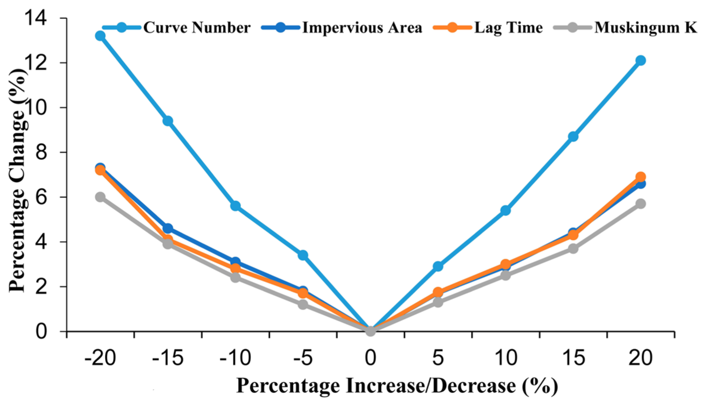
3.2. HEC-HMS Parameters Sensitivity Analysis

Model sensitivity analysis was conducted to determine which parameters of the model had a significant influence on the model output. The contribution of model parameters to an overall error in the model predictions was ranked with the aid of sensitivity analysis. Four (4) parameters of the model were subjected to sensitivity analysis. The curve number, impervious area, lag time, and Muskingum K were checked on a ±20% increment with a 5% interval. The curve number was determined to be the most sensitive parameter, as evident from Figure 5. An increase in the curve number by 20% made the peak discharge increase by 13.2%, and, when the curve number was decreased by 20%, the peak discharge was observed to decrease by 12.1%. The reason for it being the most sensitive parameter is that it depends on land use, hydrological soil groups, and antecedent moisture conditions, which are known to be the major influential factors in runoff generation. Lag time was also found to be sensitive as it tended to increase the peak discharge by 7.2% when increased by 20%, and it decreased the peak discharge by 6.8% when shortened by 20%. Figure 6 shows how these parameters deviated from the origin.

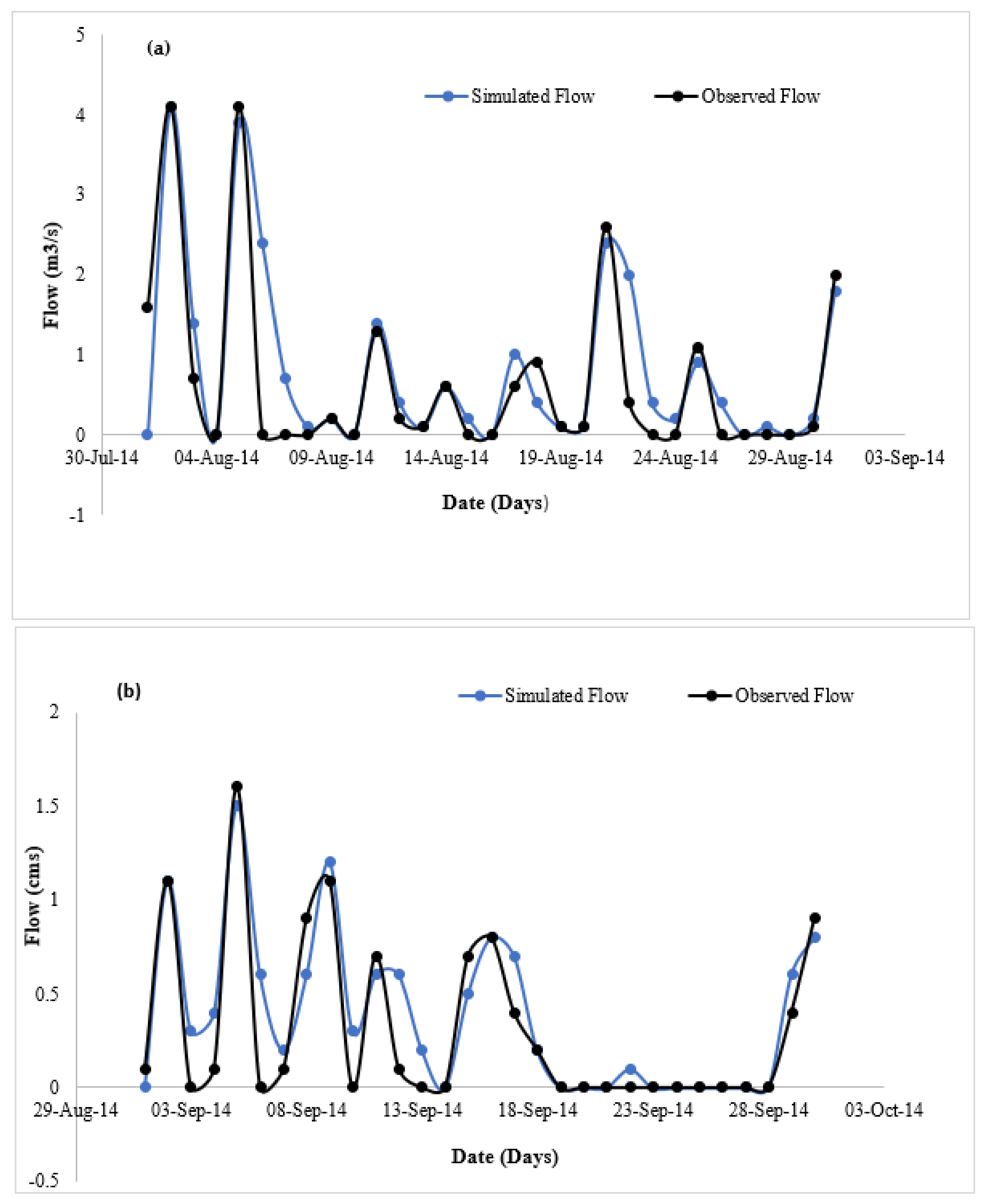
3.3. HEC-HMS Model Calibration, Validation, and Performance Evaluation

The model was found to be sensitive to curve number (CN), lag time, and Muskingum K. The HEC-HMS model calibration was achieved by auto-optimizing the sensitive parameter of the model. The parameters optimized were the curve number, lag time, and Muskingum K. The optimization operation was conducted on parameters that were sensitive to the model output.

Table 3. Initial and optimized parameters of the HEC-HMS model.

Element	Parameter	Units	Initial Value	Optimized Value
All Sub-basins	SCS Curve Number—Initial Abstraction Scale Factor		1	1.1603
All Sub-basins	SCS Curve Number—Curve Number Scale Factor		1	0.98729
W120	SCS Curve Number—Curve Number		92.66304	75.453
W110	SCS Curve Number—Curve Number		88.41209	56.694
W100	SCS Curve Number—Curve Number		89.13062	41.733
W180	SCS Curve Number—Curve Number		84.12308	84.421
W170	SCS Curve Number—Curve Number		80.13656	73.511
W160	SCS Curve Number—Curve Number		91.75	70.627
W150	SCS Curve Number—Curve Number		90.01976	63.081
W140	SCS Curve Number—Curve Number		81.43609	52.916
W130	SCS Curve Number—Curve Number		83.84741	55.924
W120	SCS Unit Hydrograph—Lag Time	MIN	16.66416	13.776
W110	SCS Unit Hydrograph—Lag Time	MIN	163.1303	156.74
W100	SCS Unit Hydrograph—Lag Time	MIN	76.08306	81.507
W180	SCS Unit Hydrograph—Lag Time	MIN	141.1654	163.75
W170	SCS Unit Hydrograph—Lag Time	MIN	79.06074	88.216
W160	SCS Unit Hydrograph—Lag Time	MIN	4.1292	4.8915
W150	SCS Unit Hydrograph—Lag Time	MIN	81.23118	100.31
W140	SCS Unit Hydrograph—Lag Time	MIN	62.38896	79.1
W130	SCS Unit Hydrograph—Lag Time	MIN	67.54464	84.897
R90	Muskingum—K	HR	0.1	0.35946
R80	Muskingum—K	HR	0.11	0.34604
R50	Muskingum—K	HR	0.11	0.2658
R40	Muskingum—K	HR	0.1	0.16622

gives the initial and optimized values of the sensitive parameters of the model.

The discharge data from August 2014 were used for the calibration, which spanned from 1 August to 31 August 2014 and showed good agreement between the simulated outflows at all junctions, including the outlet. The observed outflows that produced hydrograph shapes and the time to peak were relatively the same, as shown in Figure 6. The root mean square error standard deviation (RMSE), Nash–Sutcliffe coefficient (NSE), and percentage bias (PBIAS) before and after optimization are presented in

Table 4. Performance indices during verification.

Performance Indices	Calibration				Validation
	Before Optimization	Remark	After Optimization	Remark		Remark
RMSE	0.9	Unsatisfactory	0.6	Good	0.5	Good
NSE	0.27	Poor	0.67	Very Good	0.78	Very Good
PBIAS	50.6%	Very Poor	20.5%	Satisfactory	20.8%	Good

, while the simulated peak discharge and the total volume at the outlet were 5.3 m³/s and 583.1 mm before optimization and 4.1 m³/s and 401.7 mm after optimization. However, the performance of the model improved significantly when the RMSE, Nash–Sutcliffe coefficient, and percentage biases were within the acceptable threshold limit.

The model was validated with the daily discharge data for September 2014, which spanned from September 1 to September 30. The validation was achieved by running the calibrated model with the September 2014 (Figure 6) events. The validation shows a very close match between the observed and simulated outflows at the watershed outlet, but it slightly underestimated the peak discharge. Based on model performance indices, the result was closely similar to the result obtained in the calibration session. The RMSE, NSE, and PBIAS of the validation result were 0.50, 0.78, and 20.8%, respectively, indicating very good performance (Table 4). These results are in good agreement with those obtained by Derdour et al. [51] (who worked on the Ain Sefra watershed and the Ksour Mountains (SW Algeria)) and Khaddor et al. [57] (who modeled the Boukhalef watershed in Morocco) when using the HEC-HMS model. Moreover, other researchers used the SCS-CN method for rainfall runoff simulations, and their model performance results matched with the results obtained in this research.

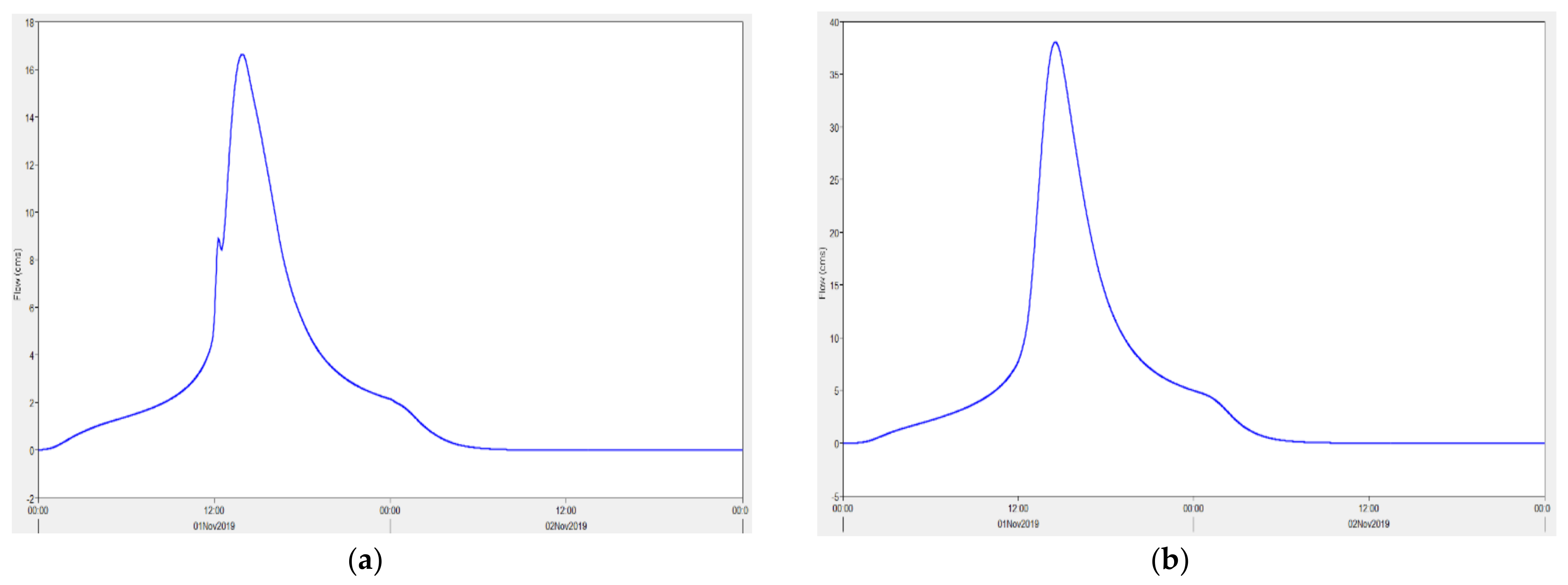
3.4. Simulation of Peak Runoff

The simulation results of the HEC-HMS model when using the frequency storm method for 2-year, 5-year, 10-year, 25-year, 50-year, 100-year, and 200-year periods at the upstream (Ganga Uku culvert), the NUGA gate culvert, towards the outlet (Dan Fodio culvert), and the watershed outlet in m³/s are presented in

Table 5. Peak discharges at a location of interest in m³/s.

	Return Periods
Location	2-Year	5-Year	10-Year	25-Year	50-Year	100-Year	200-Year
Ganga Uku (upstream)	2.9	5.4	7.1	9.4	11.1	12.8	14.6
NUGA gate culvert	3.7	6.8	9.1	12.1	14.3	16.6	19
Mid-section	5.7	11	14.9	20	23.9	27.8	31.8
Dan Fodio culvert (Towards the outlet)	6.3	12.4	16.9	22.8	27.3	31.8	36.4
Outlet	7.5	14.9	20.3	27.3	32.6	38	43.5

. It was observed from the results that the discharge increases with increased flow length. This is because of the contributions the river receives from adjacent sub-basins. For instance, the peak discharge at the NUGA gate culvert for a 50-year return period was 14.3 m³/s, which is less than the 27.3 m³/s at the Dan Fodio culvert, which is at its downstream. This is due to the fact that the stream receives runoff from Dan Fodio’s impervious surfaces through the tributary upstream of the Dan Fodio culvert. The result also follows a normal pattern of hydrological analysis, as the peak discharge was observed to increase with an increase in the return period.

The flood hydrograph for the 100-year Tr at the NUGA gate culvert and the watershed outlet are shown in Figure 7. As seen from the figure, the flood hydrographs have a shape similar to the ones obtained by Derdour et al. [51].

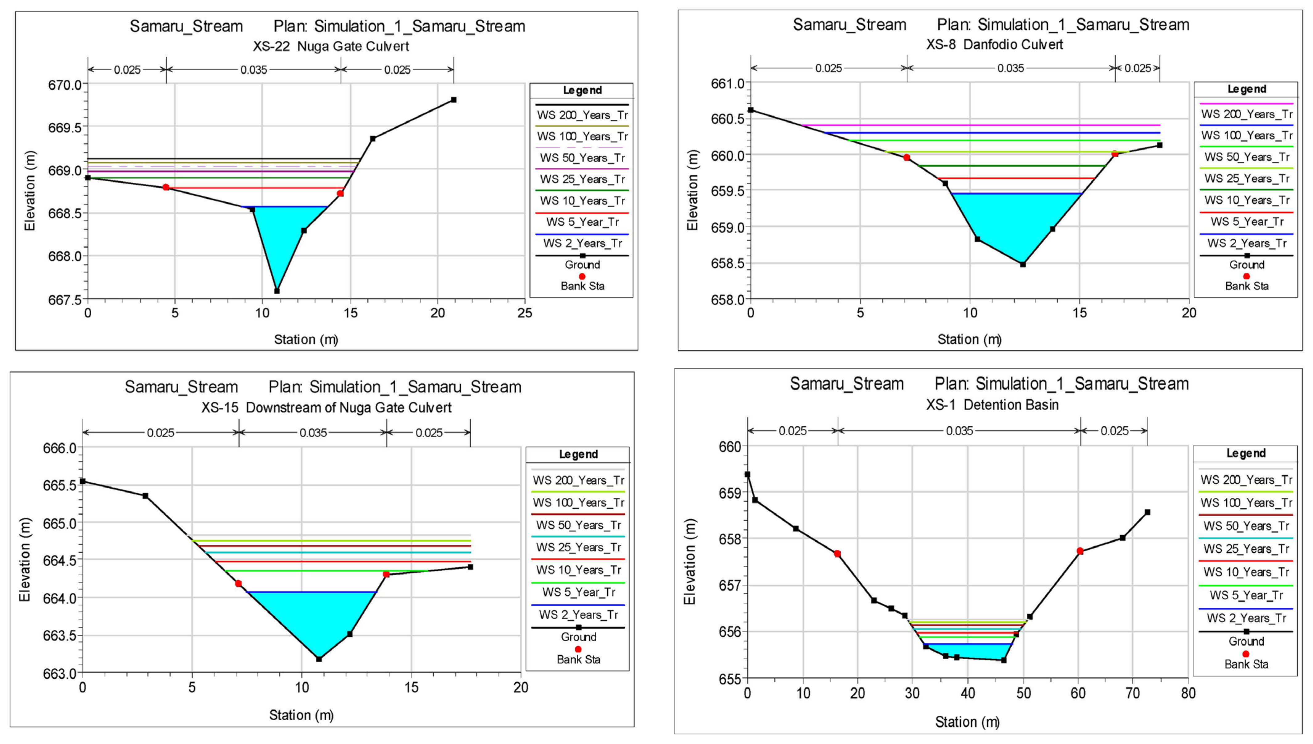
3.5. Hydraulic Evaluation of the River System of Watershed

The results for the hydraulic simulation with HE-RAS and the water surface profiles of some of the sections (where overtopping and spilling occur for flows of different return periods) were reviewed. Manning’s coefficient was not calibrated due to the lack of high-quality aerial imagery data. However, Manning’s values were carefully assigned to the main channel and the overbanks based on rigorous field observation and via consultations from literature sources.

(a)

Cross-sectional Water Surface Profile

The cross-sectional water surface profile at the NUGA gate culvert, Dan Fodio culvert, downstream of the NUGA gate culvert, and the detention basin are shown in Figure 8. As seen from the cross-section at the NUGA gate culvert (XS-22), virtually all of the flows of different return periods produced a water surface profile that overtopped the main channel and the overbanks. Hence, this signified a flash flood or overtopping of the culvert.

The culvert height was measured to be 1.24 m during a topographical survey, but the simulation results for the 2-year, 5-year, 10-year, 25-year, 50-year, 100-year, and 200-year return periods’ floods yielded water heights of 0.9 m, 1.1 m, 1.3m, 1.33 m, 1.38 m, 1.53 m, and 1.8 m, respectively. The flow characteristics at the 26 (Ganga Uku), 22 (NUGA gate culvert), 8 (Dan Fodio culvert), and 1 (Detention basin) stations for the 100-year Tr profile are shown in

Table 6. Flow characteristics at some selected river stations.

Reach	River Station	Q Total (m3/s)	Min Ch. Elv. (m)	WS. Elv. (m)	Vel. Chl. (m/s)	Flow Area (m2)	Top Width (m)	Froude No.
	Ganga Uku	12.8	675	676.2	2.6	5.0	7.4	1
Samaru Stream	NUGA gate culvert	16.5	667.6	669.1	2.3	7.7	15.5	0.9
	Dan Fodio culvert	31.3	658.5	660.3	2.9	11.6	15.3	0.87
	Detention basin	31.3	655.4	656.2	2.5	12.8	21.2	1.01

.

(b)

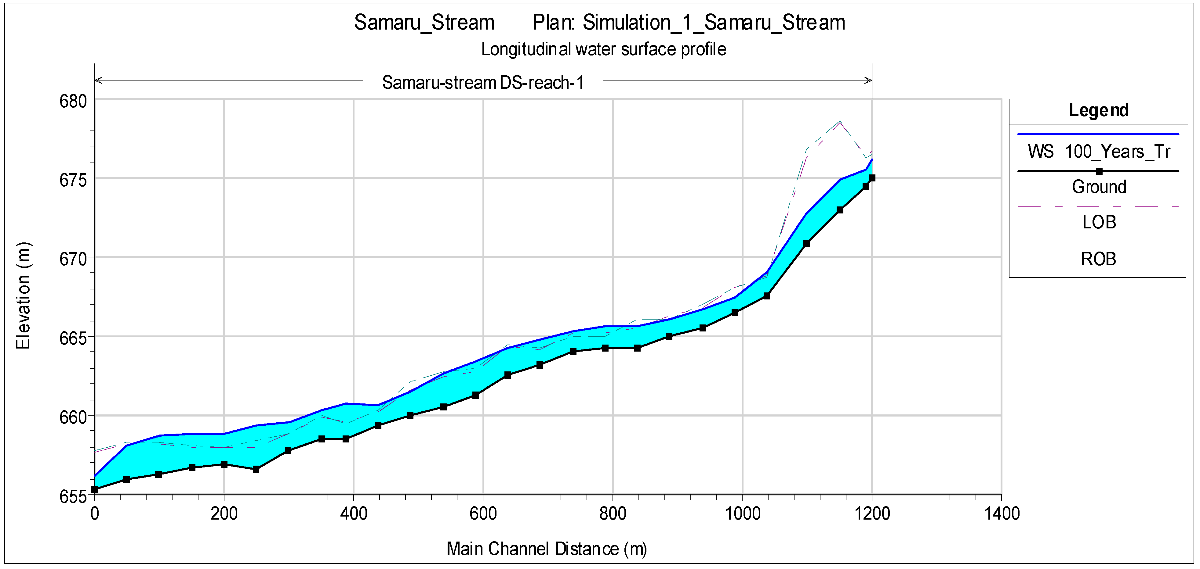
Longitudinal Water Surface Profile

The longitudinal profile shows the variation of the water surface profile for each cross-section in the channel. Figure 9 shows the longitudinal water surface profiles for the floods in a 100-year period. The profile varies significantly from section to section, as seen from the figures, and this is evident because the natural streams usually have varying cross-sections.

(c)

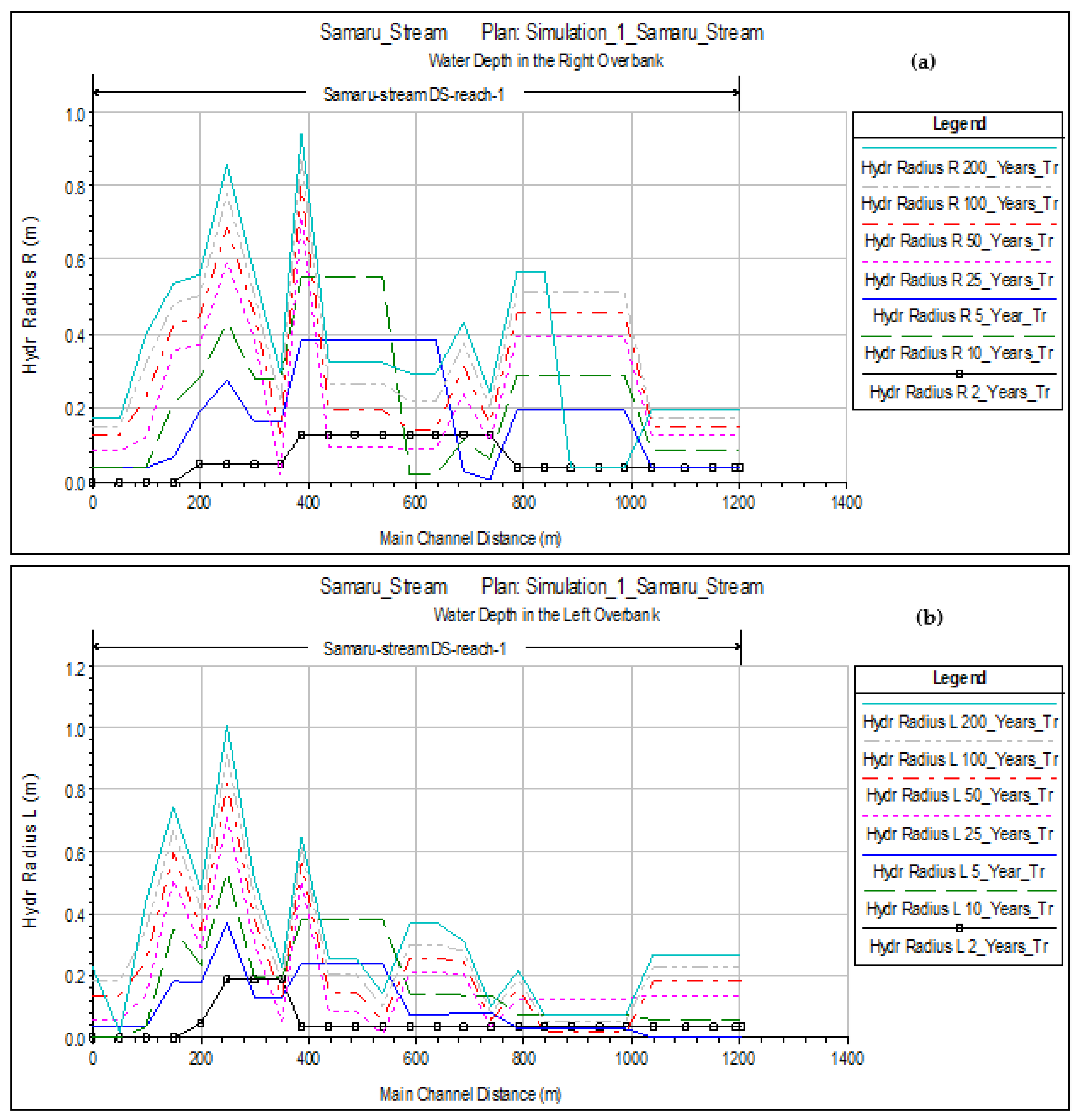
Water Depth in Overbanks

The water depth in the right and left overbanks for the different return periods is presented in Figure 10. The maximum water depth of the right overbank is about 0.9 m, while it is 1.0 m in the left overbank. Furthermore, it was observed that the water depth in both overbanks increased with an increase in the return period.

3.6. Smart Flood Control Structures

The 100-year design flood was selected along with the other basic data required for hydraulic design, such as the channel cross-section and flow characteristics. To safely convey the peak runoff from the Samaru stream watershed to the stream outlet, a hydraulically economical trapezoidal channel of a constant cross-section was designed, which was achieved by considering the peak runoff of a 100-year return period at the Dan Fodio culvert junction. The HEC-HMS model output gave the design peak discharge at the Dan Fodio culvert as 31.8 m³/s. The mean slope of the channel was obtained from the topographic survey as 0.0154. Chow [55] proposed a Manning’s coefficient for concrete as 0.012.

The channel was found to be stable after checking the value of the mean velocity to be 2.86 m/s, which falls below the allowable velocity limit for a concrete lining. Hence, the channel was deemed stable against erosion for all flow durations, which meant that the velocity was lower than the allowable velocity. The summary of the design channel is presented in

Table 7. Summary of the design channel parameters.

Channel Characteristics	Units	Symbols	Values
Normal flow depth	m	y	1.5
Bottom width	m	b	1.7
Top width	m	T	3.5
Side slope	-	z	$\raisebox{1ex}{$1$}\!\left/ \!\raisebox{-1ex}{$\sqrt{3}$}\right.$
Freeboard	m	F	0.3

.

4. Conclusions

GIS-based techniques were employed to estimate flood events in the micro-watershed of Samaru via multi-model inference. The HEC-HMS model was developed to evaluate the effect of rainfall on the peak discharges of different return periods, while the HEC-RAS model was used to analyze the water surface profiles of different return periods and their characteristics so as to develop flash flood adaptation and mitigation measures. The following conclusions were drawn from the study.

(a)

The hydrological modeling of the watershed was achieved using HEC-HMS. The intensity duration frequency curve (IDF) of the watershed was successfully developed and used for peak discharge estimation. The calibration and validation of the HEC-HMS results showed a close match between the observed and simulated flows in August and September 2014.

(b)

The calibration performance evaluation gave an RMSE, NSE, and PBIAS of 0.6, 0.67, and 20.54%, respectively, while the validation performance evaluation produces were 0.50, 0.783, and 20.77%, respectively.

(c)

A parameter sensitivity analysis of the HEC-HMS model revealed that the model outputs were more sensitive to the curve number. This may be attributed to the land use changes in the watershed, which led to increasing urbanization and paved surfaces; thus, land development in the watershed should be monitored.

(d)

The peak runoff rates from the Samaru watershed for 2-, 5-, 10-, 25-, 50-, 100-, and 200-year return periods at all junctions and reaches along the Samaru stream, including the watershed outlet, were successfully estimated. The peak discharges at the NUGA gate culvert for 2-, 5-, 10-, 25-, 50-, 100-, and 200-year return periods were estimated as 3.7, 6.8, 9.1, 12.1, 14.3, 16.6, and 19.0 m³/s, respectively, while those at the watershed outlet were found to be 5.7, 11.0, 14.9, 20.0, 23.9, 27.8, and 31.8 m³/s, respectively.

(e)

The hydraulic modeling of the Samaru stream was performed using the HEC-RAS model with river cross-sections; the flow data from the 2-, 5-, 10-, 25-, 50-, 100-, and 200-year return periods; and Manning’s coefficient as the input data. The modeling analysis yielded water depth, water velocity, and other flow characteristics at all of the cross-sections that were entered for the respective return periods.

(f)

The floods of the 25-year return period and above produced water surface profiles that inundated the overbanks at cross-sections 22, 24, 9, and 8. Furthermore, the NUGA gate culvert was also found to be overtopped by floods in 25-year return periods and above.

(g)

The maximum water depth in the right and left overbanks was found to be about 0.9 m and 1.0 m, respectively. This was used for channel design, which was achieved by considering the floods in a 100-year return period. The most economical channel section design gave approximate channel dimensions of 1.50 m as the normal flow depth, 1.73 m as the bottom width, 3.50 m as the channel top width, and a free board of 0.30 m.

(h)

These findings enable an improved understanding of parameter behavior in the HEC-HMS model application, as well as aids in the identification of the dominant processes under different hydrological scenarios that will allow for the accurate estimation of floods in micro-watersheds.

References

1. Nabinejad, S.; Schüttrumpf, H. Flood Risk Management in Arid and Semi-Arid Areas: A Comprehensive Review of Challenges, Needs, and Opportunities. Water 2023, 15, 3113. [Google Scholar] [CrossRef]
2. Subraelu, P.; Ahmed, A.; Ebraheem, A.A.; Sherif, M.; Mirza, S.B.; Ridouane, F.L.; Sefelnasr, A. Risk Assessment and Mapping of Flash Flood Vulnerable Zones in Arid Region, Fujairah City, UAE-Using Remote Sensing and GIS-Based Analysis. Water 2023, 15, 2802. [Google Scholar] [CrossRef]
3. Mishra, K.; Sinha, R. Flood risk assessment in the Kosi megafan using multi-criteria decision analysis: A hydro-geomorphic approach. Geomorphology 2020, 350, 106861. [Google Scholar] [CrossRef]
4. Pinos, J.; Quesada-Román, A. Flood Risk-Related Research Trends in Latin America and the Caribbean. Water 2022, 14, 10. [Google Scholar] [CrossRef]
5. Quesada-Román, A. Disaster Risk Assessment of Informal Settlements in the Global South. Sustainability 2022, 14, 10261. [Google Scholar] [CrossRef]
6. Shuaibu, A.; Hounkpè, J.; Bossa, Y.A.; Kalin, R.M. Flood Risk Assessment and Mapping in the Hadejia River Basin, Nigeria, Using Hydro-Geomorphic Approach and Multi-Criterion Decision-Making Method. Water 2022, 14, 3709. [Google Scholar] [CrossRef]
7. Khosravi, K.; Pham, B.T.; Chapi, K.; Shirzadi, A.; Shahabi, H.; Revhaug, I.; Prakash, I.; Bui, D.T. A comparative assessment of decision trees algorithms for flash flood susceptibility modeling at Haraz watershed, northern Iran. Sci. Total Environ. 2018, 627, 744–755. [Google Scholar] [CrossRef]
8. Abdulrahman, S.; Bwambale, J. A review on flood risk assessment using multicriteria decision making technique. World Water Policy 2021, 7, 209–221. [Google Scholar] [CrossRef]
9. Alfa, M.I.; Ajibike, M.A.; Daffi, R.E. Application of Analytic Hierarchy Process and Geographic Information System Techniques in Flood Risk Assessment: A Case of Ofu River Catchment in Application of analytic hierarchy process and geographic information system techniques in flood risk assessm. J. Degrad. Min. Lands Manag. 2018, 5, 1363–1372. [Google Scholar] [CrossRef]
10. Echendu, A.J. The impact of flooding on Nigeria’s sustainable development goals (SDGs). Ecosyst. Health Sustain. 2020, 6, 1791735. [Google Scholar] [CrossRef]
11. Echendu, A.J. Flooding in Nigeria and Ghana: Opportunities for partnerships in disaster-risk reduction. Sustain. Sci. Pract. Policy 2022, 18, 1–15. [Google Scholar] [CrossRef]
12. Umar, N.; Gray, A. Flooding in Nigeria: A review of its occurrence and impacts and approaches to modelling flood data. Int. J. Environ. Stud. 2022, 80, 540–561. [Google Scholar] [CrossRef]
13. Oyedele, P.; Kola, E.; Olorunfemi, F.; Walz, Y. Understanding Flood Vulnerability in Local Communities of Kogi State, Nigeria, Using an Index-Based Approach. Water 2022, 14, 2746. [Google Scholar] [CrossRef]
14. Dorcas, I.; Wendy, Z. Land Use and Land Cover Change Assessment in the Context of Flood Hazard in Lagos State, Nigeria. Water 2021, 13, 1105. [Google Scholar] [CrossRef]
15. Cirella, G.T.; Iyalomhe, F.O. Flooding Conceptual Review: Sustainability-Focalized Best Practices in Nigeria. Appl. Sci. 2018, 8, 1558. [Google Scholar] [CrossRef]
16. Oladokun, V.; Proverbs, D. Flood risk management in Nigeria: A review of the challenges and opportunities. Int. J. Saf. Secur. Eng. 2016, 6, 485–497. [Google Scholar] [CrossRef]
17. Miguez, M.G.; Battemarco, B.P.; De Sousa, M.M.; Rezende, O.M.; Veról, A.P.; Gusmaroli, G. Urban Flood Simulation Using MODCEL—An Alternative Quasi-2D Conceptual Model. Water 2017, 9, 445. [Google Scholar] [CrossRef]
18. Xiao, H.; Vasconcelos, J.G. Evaluating Curve Number Implementation Alternatives for Peak Flow Predictions in Urbanized Watersheds Using SWMM. Water 2022, 15, 41. [Google Scholar] [CrossRef]
19. Kurki-Fox, J.J.; Doll, B.A.; Line, D.E.; Baldwin, M.E.; Klondike, T.M.; Fox, A.A. Estimating Changes in Peak Flow and Associated Reductions in Flooding Resulting from Implementing Natural Infrastructure in the Neuse River Basin, North Carolina, USA. Water 2022, 14, 1479. [Google Scholar] [CrossRef]
20. Ran, L.; Wang, S.; Lu, X.X. Hydraulic geometry change of a large river: A case study of the upper Yellow River. Environ. Earth Sci. 2011, 66, 1247–1257. [Google Scholar] [CrossRef]
21. Feng, B.; Zhang, Y.; Bourke, R. Urbanization impacts on flood risks based on urban growth data and coupled flood models. Nat. Hazards 2021, 106, 613–627. [Google Scholar] [CrossRef]
22. McGrane, S.J. Impacts of urbanisation on hydrological and water quality dynamics, and urban water management: A review. Hydrol. Sci. J. 2016, 61, 2295–2311. [Google Scholar] [CrossRef]
23. Mizuki, C.; Kuzuha, Y. Frequency Analysis of Hydrological Data for Urban Floods—Review of Traditional Methods and Recent Developments, Especially an Introduction of Japanese Proper Methods. Water 2023, 15, 2490. [Google Scholar] [CrossRef]
24. Nugent, J.L. A Comparison of Manual and Geographic Information System Techniques for Environmental Planning Mapping and Analysis; State University of New York: New York, NY, USA, 1991. [Google Scholar]
25. Deshpande, S.S. Improved Floodplain Delineation Method Using High-Density LiDAR Data. Comput. Civ. Infrastruct. Eng. 2012, 28, 68–79. [Google Scholar] [CrossRef]
26. Jafarzadegan, K.; Merwade, V. A DEM-based approach for large-scale floodplain mapping in ungauged watersheds. J. Hydrol. 2017, 550, 650–662. [Google Scholar] [CrossRef]
27. Sindhu, K.; Rao, D. Hydrological and hydrodynamic modeling for flood damage mitigation in Brahmani—Baitarani River Basin, India. Geocarto Int. 2017, 32, 1004–1016. [Google Scholar] [CrossRef]
28. Boutaghane, H.; Boulmaiz, T.; Lameche, E.K.; Lefkir, A.; Hasbaia, M.; Abdelbaki, C.; Moulahoum, A.W.; Keblouti, M.; Bermad, A. Flood Analysis and Mitigation Strategies in Algeria. In Wadi Flash Floods: Challenges and Advanced Approaches for Disaster Risk Reduction; Springer: Cham, Switzerland, 2022. [Google Scholar] [CrossRef]
29. El-Naqa, A.; Jaber, M. Floodplain Analysis using ArcGIS, HEC-GeoRAS and HEC-RAS in Attarat Um Al-Ghudran Oil Shale Concession Area, Jordan. J. Civ. Environ. Eng. 2018, 8, 1–11. [Google Scholar] [CrossRef]
30. Grimaldi, S.; Schumann, G.J.; Shokri, A.; Walker, J.P.; Pauwels, V.R.N. Challenges, Opportunities, and Pitfalls for Global Coupled Hydrologic-Hydraulic Modeling of Floods. Water Resour. Res. 2019, 55, 5277–5300. [Google Scholar] [CrossRef]
31. Zeleňáková, M.; Fijko, R.; Labant, S.; Weiss, E.; Markovič, G.; Weiss, R. Flood risk modelling of the Slatvinec stream in Kružlov village, Slovakia. J. Clean. Prod. 2018, 212, 109–118. [Google Scholar] [CrossRef]
32. Plate, E.J. Flood risk and flood management. J. Hydrol. 2002, 267, 2–11. [Google Scholar] [CrossRef]
33. Şen, Z. Flood Modeling, Prediction and Mitigation; Springer Science and Business Media LLC.: Dordrecht, The Netherlands, 2018; ISBN 9783319523552. [Google Scholar]
34. Nharo, T.; Makurira, H.; Gumindoga, W. Mapping floods in the middle Zambezi Basin using earth observation and hydrological modeling techniques. Phys. Chem. Earth Parts A/B/C 2019, 114, 102787. [Google Scholar] [CrossRef]
35. Natarajan, S.; Radhakrishnan, N. An Integrated Hydrologic and Hydraulic Flood Modeling Study for a Medium-Sized Ungauged Urban Catchment Area: A Case Study of Tiruchirappalli City Using HEC-HMS and HEC-RAS. J. Inst. Eng. Ser. A 2020, 101, 381–398. [Google Scholar] [CrossRef]
36. Xiao, B.; Wang, Q.-H.; Fan, J.; Han, F.-P.; Dai, Q.-H. Application of the SCS-CN Model to Runoff Estimation in a Small Watershed with High Spatial Heterogeneity. Pedosphere 2011, 21, 738–749. [Google Scholar] [CrossRef]
37. Abdessamed, D.; Abderrazak, B. Coupling HEC-RAS and HEC-HMS in rainfall–runoff modeling and evaluating floodplain inundation maps in arid environments: Case study of Ain Sefra city, Ksour Mountain. SW of Algeria. Environ. Earth Sci. 2019, 78, 586. [Google Scholar] [CrossRef]
38. Laouacheria, F.; Mansouri, R. Comparison of WBNM and HEC-HMS for Runoff Hydrograph Prediction in a Small Urban Catchment. Water Resour. Manag. 2015, 29, 2485–2501. [Google Scholar] [CrossRef]
39. Bruno, L.S.; Mattos, T.S.; Oliveira, P.T.S.; Almagro, A.; Rodrigues, D.B.B. Hydrological and Hydraulic Modeling Applied to Flash Flood Events in a Small Urban Stream. Hydrology 2022, 9, 223. [Google Scholar] [CrossRef]
40. Garba, M.L.; Yusuf, Y.O.; Arabi, A.S.; Musa, S.K.; Schoeneich, K. An Update on the quality of water in Samaru Stream. Zaria Geogr. 2014, 21, 75–84. [Google Scholar]
41. Shehu, J.; Yusuf, Y.O.; Koki, I.B. Dissolved Sediment Delivery by the Samaru Stream into the Ahmadu Bello University Reservior, Zaria, Nigeria. J. Nat. Sci. Res. 2016, 6, 16–22. [Google Scholar]
42. Youssef, A.M.; Hegab, H.A. Flood-Hazard Assessment Modeling Using Multicriteria Analysis and GIS: A Case Study—Ras Gharib Area, Egypt, No. 2017; Elsevier Inc.: Amsterdam, The Netherlands, 2019. [Google Scholar] [CrossRef]
43. Zakaria, S.; Mustafa, Y.T.; Mohammed, D.A.; Ali, S.S.; Al-Ansari, N.; Knutsson, S. Estimation of annual harvested runoff at Sulaymaniyah Governorate, Kurdistan region of Iraq. Nat. Sci. 2013, 05, 1272–1283. [Google Scholar] [CrossRef]
44. Al Mamun, A.; bin Salleh, N.; Noor, H.M. Estimation of short-duration rainfall intensity from daily rainfall values in Klang Valley, Malaysia. Appl. Water Sci. 2018, 8, 203. [Google Scholar] [CrossRef]
45. Sam, M.G.; Nwaogazie, I.L.; Ikebude, C.; Inyang, U.J.; Irokwe, J.O. Modeling Rainfall Intensity-Duration-Frequency (IDF) and Establishing Climate Change Existence in Uyo-Nigeria Using Non-Stationary Approach. J. Water Resour. Prot. 2023, 15, 194–214. [Google Scholar] [CrossRef]
46. Bibi, T.S.; Tekesa, N.W. Impacts of climate change on IDF curves for urban stormwater management systems design: The case of Dodola Town, Ethiopia. Environ. Monit. Assess. 2022, 195, 1–17. [Google Scholar] [CrossRef]
47. Halder, A.; Majed, N. The effects of unplanned land use and heavy seasonal rainfall on the storm-water drainage in Dhaka metropolitan city of Bangladesh. Urban Water J. 2023, 20, 707–722. [Google Scholar] [CrossRef]
48. Haddad, K.; Rahman, A. Derivation of short-duration design rainfalls using daily rainfall statistics. Nat. Hazards 2014, 74, 1391–1401. [Google Scholar] [CrossRef]
49. Bhagat, N. Flood Frequency Analysis Using Gumbel’s Distribution Method: A Case Study of Lower Mahi Basin, India. J. Water Resour. Ocean Sci. 2017, 6, 51. [Google Scholar] [CrossRef]
50. Onen, F.; Bagatur, T. Prediction of Flood Frequency Factor for Gumbel Distribution Using Regression and GEP Model. Arab. J. Sci. Eng. 2017, 42, 3895–3906. [Google Scholar] [CrossRef]
51. Derdour, A.; Bouanani, A.; Babahamed, K. Modelling rainfall runoff relations using HEC-HMS in a semi-arid region: Case study in Ain Sefra watershed, Ksour Mountains (SW Algeria). J. Water Land Dev. 2018, 36, 45–55. [Google Scholar] [CrossRef]
52. Howard, D.A.; Luzzadder-Beach, S.; Beach, T. Field evidence and hydraulic modeling of a large Holocene jökulhlaup at Jökulsá á Fjöllum channel, Iceland. Geomorphology 2012, 147–148, 73–85. [Google Scholar] [CrossRef]
53. Barnes, H.H. Roughness Characteristics of Natural Channels; US Government Printing Office: Washington, DC, USA, 1967; Volume 1849.
54. USACE. “HEC-RAS Hydraulic Reference Manual”. p. 464. 2016. Available online: https://www.hec.usace.army.mil/software/hec-ras/documentation/HEC-RAS%205.0%20Reference%20Manual.pdf (accessed on 23 November 2023).
55. Akan, A.O. Open Channel Hydraulics; Elsevier: Amsterdam, The Netherlands, 2006; ISBN 9780128217702. [Google Scholar]
56. Muhammad, M.M.; Petronas, U.T.; Yusof, K.W.; Mustafa, M.R.U.; Ghani, A.A. Velocity Distributions in Grassed Channel. In Proceedings of the 4th Annual International Conference on Architecture and Civil Engineering (ACE 2016), Singapore, 25–26 April 2016. [Google Scholar]
57. Khaddor, I.; Achab, M.; Soumali, M.R.; Alaoui, A.H. Rainfall-runoff calibration for semi-arid ungauged basins based on the cumulative observed hyetograph and SCS storm model: Application to the Boukhalef watershed (Tangier, North Western Morocco). J. Mater. Environ. Sci. 2017, 8, 3795–3808. [Google Scholar]
Figure 1. Location of the Samaru stream watershed on a Nigerian map.
Water 15 04201 g001
Figure 2. Characteristics of the Samaru watershed. (a) Land use of the study area, (b) slope, (c) hydrological soil map, and (d) curve number grid.
Water 15 04201 g002
Figure 3. Flow chart of the methodology.
Water 15 04201 g003
Figure 4. The IDF curve of the Samaru watershed.
Water 15 04201 g004
Figure 5. Sensitivity analysis on a 100−year return period simulation.
Water 15 04201 g005
Figure 6. Simulated and observed hydrographs: (a) the calibration and (b) validation.
Water 15 04201 g006
Figure 7. Flood hydrograph of the 100−year Tr at (a) the NUGA gate culvert and (b) the watershed outlet.
Water 15 04201 g007
Figure 8. Cross-sectional profile at the NUGA gate culvert, Dan Fodio culvert, downstream of the NUGA gate Culvert, and the detention basin.
Water 15 04201 g008
Figure 9. Longitudinal water surface profile for floods in a 100-year period.
Water 15 04201 g009
Figure 10. Water depth in (a) the right overbank and (b) the left overbank.
Water 15 04201 g010