Article

Performance of LSTM over SWAT in Rainfall-Runoff Modeling in a Small, Forested Watershed: A Case Study of Cork Brook, RI

by
Shiva Gopal Shrestha
and
Soni M. Pradhanang
*
Department of Geosciences, University of Rhode Island, Kingston, RI 02881, USA
*
Author to whom correspondence should be addressed.
Water 2023, 15(23), 4194; https://doi.org/10.3390/w15234194
Submission received: 27 October 2023 / Revised: 28 November 2023 / Accepted: 30 November 2023 / Published: 4 December 2023

Abstract

:
The general practice of rainfall-runoff model development towards physically based and spatially explicit representations of hydrological processes is data-intensive and computationally expensive. Physically based models such as the Soil Water Assessment tool (SWAT) demand spatio-temporal data and expert knowledge. Also, the difficulty and complexity is compounded in the smaller watershed due to data constraint and models’ inability to generalize hydrologic processes. Data-driven models can bridge this gap with their mathematical formulation. Long Short-Term Memory (LSTM) is a data-driven model with Recurrent Neural Network (RNN) architecture, which is better suited to solve time series problems. Studies have shown that LSTM models have competitive performance in watershed hydrology studies. In this study, a comparative analysis of SWAT and LSTM models in the Cork Brook watershed shows that results from LSTM were competitive to SWAT in flow prediction with NSE of 0.6 against 0.63, respectively, given the limited availability of data. LSTM models do not overestimate the high flows like SWAT. However, both these models struggle with low values estimation. Although interpretability, explainability, and use of models across different datasets or events outside of the training data may be challenging, LSTM models are robust and efficient.

1. Introduction

The history of rainfall–runoff modeling is among the oldest yet evolving in hydrological sciences. Initially, attempts were made to simulate and predict discharge based on precipitation events using regression-based approaches dating back over a century [1]. Physically based concepts, formulations, and algorithms followed this development. However, as computational technology and high-resolution spatial and temporal data availability advanced, the modeling concepts evolved to incorporate physically based processes and spatiotemporal variability of catchments enabling more accurate representations of hydrological processes [1,2,3,4].
Despite the progress in physically based modeling, its application in operational rainfall–runoff forecasting remains limited owing to the main challenges posed due to high computational costs and the extensive meteorological data requirements [5]. This limitation has led to the continued use of simplified physically based or conceptual models for operational purposes [6,7,8]. The major hurdle caused by high computational cost becomes more cumbersome when multi-model runs, and uncertainty analysis are to be incorporated. However, data-based modeling approaches, such as regression and artificial neural networks (ANNs), have been explored as viable alternatives to bridge the complexity posed by physically based approaches [9,10,11].
Among these alternatives, ANNs have gained significant attention due to their ability to effectively mimic highly non-linear and complex systems. Early studies in the 1990s demonstrated the potential of ANNs for rainfall–runoff prediction, and since then, they have been widely applied in hydrological modeling [12]. However, traditional feed-forward ANNs have limitations in handling time series data as they do not retain information about the sequential order of inputs. To overcome this limitation, recurrent neural networks (RNNs) were introduced. RNNs are a specialized type of neural network architecture designed to understand temporal dynamics by processing inputs in their sequential order. Using RNNs for rainfall–runoff modeling has demonstrated their potential for event-based applications [13].
Further advancements in neural network architecture led to the development of Long Short-Term Memory (LSTM) networks, which excel in capturing long-term dependencies and storage effects within the hydrological catchments [14,15,16]. LSTM was introduced to address the limitations of traditional RNNs, making them more suitable for problems where the sequential order of inputs matters [17]. In recent years, deep neural networks, including LSTM-based models, have gained traction in water quantity and quality due to their capacity to leverage big data [18]. Researchers have increasingly utilized these models to simulate rainfall–runoff relationships and improve water resources and flood management. As data availability and computing power continue to grow, the application of ANN models in hydrological sciences is expected to advance further, enabling more accurate and reliable predictions of rainfall–runoff processes [4,15,19].
In recent years, deep learning, particularly through neural networks, has garnered significant attention and success in various fields, including hydrological modeling. While deep learning is well-known for its applications in computer vision, speech recognition, and natural language processing, researchers have explored its potential in hydrological problems. LSTM has shown promise in various hydrological applications The research conducted in precipitation nowcasting, soil moisture prediction, water quality, and stream flow predictions show that deep learning has had large success and generated huge interest in hydrological sciences recently [4,18,20,21,22,23]. These studies have shown the predictive capacity of such model par with the current state-of-the-art hydrological models [14,24,25,26]. These advancements are largely facilitated by improvements in computer technology, especially through graphic processing units, and the availability of vast datasets. Moreover, the increasing popularity is attributed to solving environmental problems due to their ability to handle highly nonlinear challenges without requiring knowledge of physical processes and often large volumes of data [14,26,27].
Various studies have evaluated the effectiveness of ANN models in predicting water quantity. Still, they come with challenges, such as determining the optimal network structure through trial and error and selecting the best input variables [8,17,28]. Extrapolation beyond the training data range can also lead to significant errors, and ML-based models may need help to capture the impact of changing land use in watersheds [29]. In recent hydrological studies, recurrent neural networks and long short-term memory networks have gained momentum due to their ability to handle time series data effectively [4,13,26]. RNNs have loops that allow information from previous time steps to be passed to the next, making them suitable for time-dependent data [13]. However, the vanishing or exploding gradient problem hampers their ability to learn long-term dependencies [30]. LSTM networks were developed to overcome this issue, allowing them to effectively learn long-term dependencies in the data series [31].
Despite the successes, there is still a need to understand how LSTM structures and parameters affect predictive accuracy in different hydrological contexts [9,32]. Research in this area is ongoing, and applying deep learning approaches, especially LSTM, holds promise for advancing hydrological modeling and improving our understanding of complex hydrological phenomena [16,33]. In addition to the applications of deep learning in hydrological modeling, it is worth noting that regardless of the modeling approach used, models are typically calibrated for specific catchments where observed time series of meteorological and hydrological data are available [34]. Predictions in ungauged regions have shown decreased performance [19]. The calibrated model and parameter are localized or need explainability for the usability field [19,33,35]. Moreover, the calibration process is essential because models are simplified representations of real catchment hydrology, and parameters must effectively represent hydrological processes and address hydrologic behavior and catchment characteristics [1,36].
Although SWAT is very popular in hydrological studies, the inference of performance has largely been drawn from a couple of goodness of fit measures like the Nash–Sutcliffe model efficiency coefficient (NSE) and Coefficient of Determination (R2) [37]. In this study, a case study was conducted to investigate the performance of SWAT and LSTM in a small undisturbed forested watershed with limited data in Rhode Island. Apart from the frequently used goodness of fit measures, model results were compared against various percentiles of flows and flow duration curve (FDC) signature indices for a better assessment of model performance. Further developments in this approach can lead to in-depth analysis for water quality modeling and climate change impact assessment.

2. Materials and Methods

2.1. Study Area

The study area is Cork Brook in Scituate, Rhode Island, USA. It is a small, forested, and pristine watershed with a 7 sq km area contributing to the Scituate Reservoir (Figure 1 and Figure 2). The Scituate Reservoir is a large reservoir serving as a drinking water source to Providence. The main land use of the study area is undeveloped forest covering 79% of the area and brushland, where 14% of land use is classified as medium-density residential [38]. The soil in this area is mainly coarse-loamy, mixed, mesic Typic Dystrudept [39].
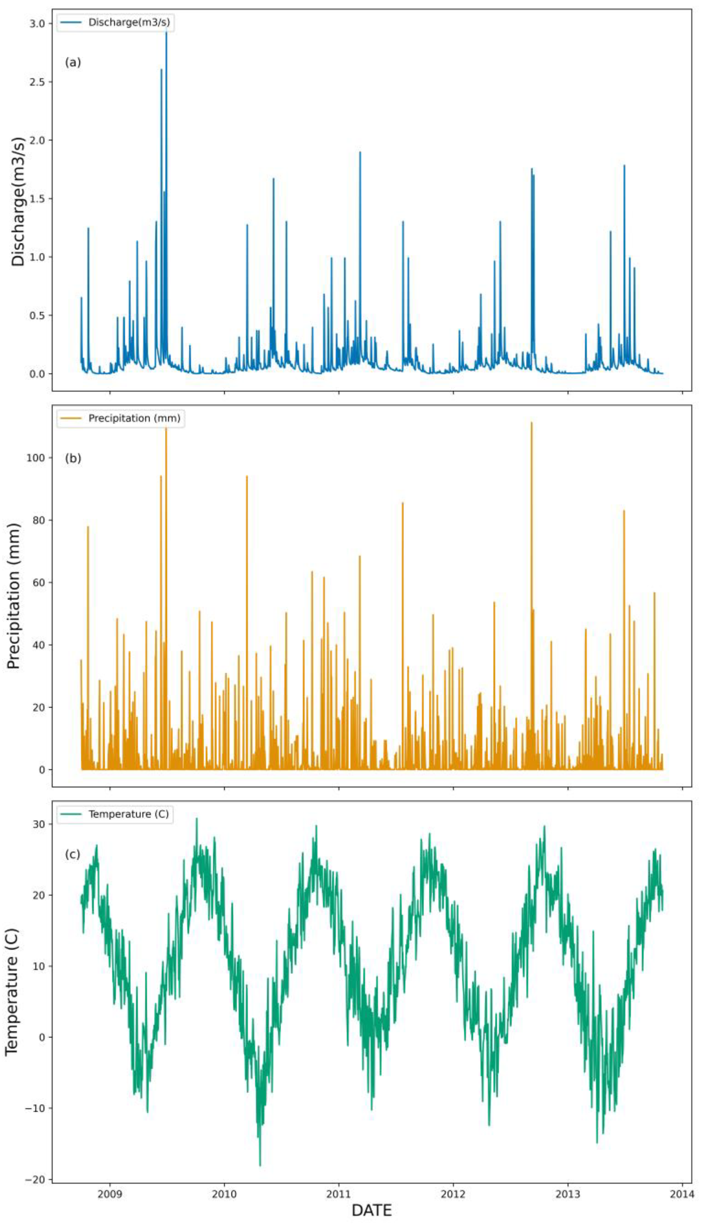
The climate of the study area consists of a humid continental climate with warm summers and cold winters with a mix of rain and snow in the form of precipitation. The meteorological forcing data used here are daily rainfall and average daily temperature from 2009–2014 from the Parameter-elevation Regressions on the Independent Slopes Model (PRISM), and daily discharge data for the same period is used from USGS station 01115280. The watershed has an annual average discharge of 0.0914 m3/s, an average annual precipitation of around 1380 mm, and an average daily temperature of around 9.6 °C since 2001. The discharge is characterized by flood events in winter, mainly in March and December, and a low-flow period in summer months from July to October. There is uniformity and coherence in the observed flow and meteorological data with high flows matching high precipitation events (Figure 3).

2.2. Model

2.2.1. SWAT

The SWAT model is a physically based hydrological model developed by the U.S. Department of Agriculture and the Agricultural Research Service [40]. It represents the hydrologic process at hydrological response units, which are the building blocks of watersheds representing similar land use, soil type, and elevation class. The SWAT model has a strong conceptual and physical understanding of watershed processes and the explainability of parameters. Numerous studies have been conducted using the application of SWAT in forested watersheds [41,42,43]. In this study, the SWAT model is calibrated using the Uncertainty in Sequential Uncertainty Fitting (SUFI) in SWATCUP, a Calibration Uncertainty Procedure program, which has the ability for sensitivity analysis, calibration, validation, and uncertainty analysis of the SWAT model [44].
The SWAT model uses the soil water equation to simulate the water balance of a watershed.
SW t =   SW o + i = 1 t   ( P i R i ET i W i Q i )
where SWt is the resultant soil water content from SW0 which is the initial soil water content, t is time (days), Pi is the amount of precipitation(mm), Ri is the amount of surface runoff (mm), ETi is the amount of evapotranspiration (mm), Wi is the percolation of water the soil profile (mm), and Qi is the amount of return flow all at the same daily time step.
The spatio-temporal data requirements of SWAT are generally topography, soil characteristics, land cover or land use, and meteorological data. In this study land use was retrieved from 2011 statewide 10-m resolution National Land Cover Data imagery [38]; soil data were retrieved from a soil map from the Natural Resource Conservation Service (NRCS) Soil Survey Geographic database (SSURGO); and topographical data was retrieved from USGS 7.5-min digital elevation models (DEMs) with a 10-m resolution. These spatial data were sourced from a public database called the Rhode Island Geographic Information System (RIGIS) database. Gridded PRISM meteorological data from 2009 to 2014 was used as temporal data as the USGS gauge has flow records starting only from 2009. SWAT employs the spatial data to create subbasin and HRU units. The Cork Brook SWAT model consists of seven subbasins and 60 HRUs using land, soil, and slope thresholds of 20%, 10%, and 5%.

2.2.2. LSTM

LSTM’s structure is developed based on recurrent neural networks. RNN has an architecture with a feedback loop that simulates time series data. However, it cannot remember longer dependencies. In contrast to RNN, LSTM employs gates and cell states which addresses challenge of the remembering long-term dependencies and gradient explosion [31]. This robustness introduced in the algorithm enables LSTM to model processes with long-term dependencies like snow moisture groundwater recharges and enables its robust prediction algorithm to be better suited to time series data [45].
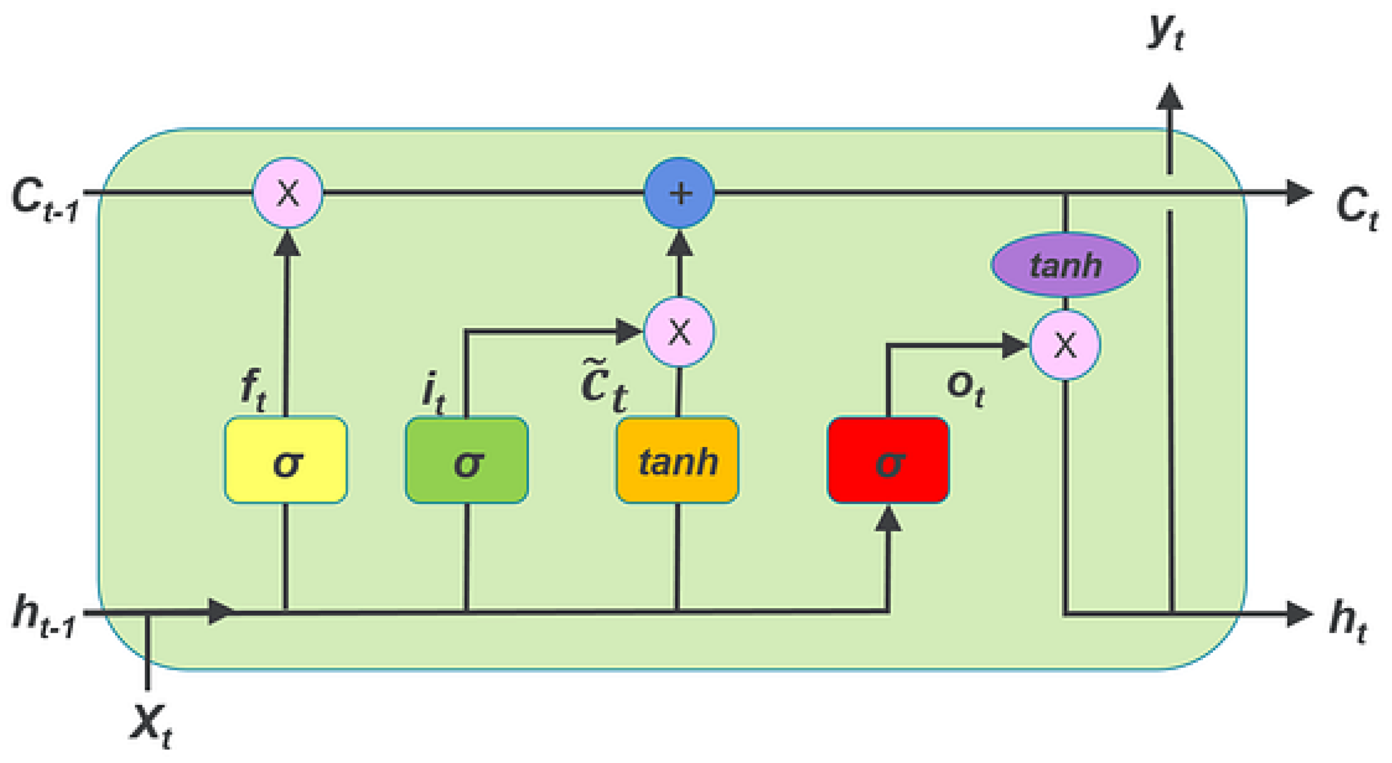
An LSTM network consists of an input layer for input sequence data, the fully connected layer that feeds input data to LSTM cells, the LSTM cell layer acting memorizing cells, and output layers that result in an output vector. In the LSTM architecture, the main elements are fully connected layers and LSTM cells [46]. Within each LSTM layer, there are two main states, the cell state and the hidden state which are carried over to the next steps (Figure 4) [47]. These memory states are responsible for remembering the model learnings. Three major gates namely input, output, and forget gates are used to manipulate this memory. Forget and input gates update the cell state and output gate updates the hidden state at each sequence.
Rewriting these into equations, LSTM has 3 gates: input, output, forget gate, cell state, and hidden states. The equation of gates is as follows:
it = σ (wi[ht−1,xt] + bi)
ft = σ (wf[ht−1,xt] + bf)
ot = σ (wo[ht−1,xt] + bo)
Čt = tanh(wc[ht−1,xt] + bc)
C t = f t   ×   C t 1   +   i t   ×   Č t
h t = o t   ×   tanh ( C t )
where it, ft and ot are input, forget, and output gates, wt weight matrix at each gate, ht−1 is the output of each previous block, xt is input, bx are biases of each gate(x), Ct are cell state at t, and Čt candidate for cell state, σ is the sigmoid function; tanh is the hyperbolic tangent function.
After the forward propagation process, the backpropagation algorithm updates the parameters and optimizes the model. In this study, observed flow data are used as targets to evaluate the loss values of the simulated flows by the LSTM network, and the Adam algorithm was proposed and applied to optimize and update the network weights.

2.2.3. Methodology

The main steps in building the LSTM model are (a) feature selection and data preprocessing (b) LSTM model structure hyperparameters tuning (c) model evaluation.

2.2.4. Feature Selection and Data Preprocessing

To set up the model, the data from 2009–2014 was split into 70% training data and 30% test data. Data splitting is a common practice to evaluate model performance and avoid overfitting. This was kept uniform for SWAT as well.
Also, for the LSTM model, the training data are manipulated by varying the time lags of the stream flow to find the best feed for the subset of features. As this is closely linked to the autocorrelation in the data, this is tuned as a parameter to train the model. It varied from 3 days to 365 days and the best values were chosen from optimization.
The data is further transformed by scaling and normalization which is a key pre-processing step in deep learning models. Normalization is a generally used transformation method that transforms the data between a standard range of zero and one. In this study, the MinMax Scaler was used to subtract the minimum values in the feature and divide by the range of the original data. This helps to balance the impact of variables and helps aid the performance of the algorithm [14,49].

2.2.5. LSTM Model Structure and Hyperparameter Tuning

The model structure of a neural network is complicated as there is no established approach to define the hydrological system. This necessitates the use of hit and trial over different model structures and configurations that can mimic a hydrological system. LSTM model structure was composed of five neural network layers and two dense layers with Adam as the model optimizer and mean square error as the loss function. Moreover, we used a regularization method as early stopping and dropout to reduce overfitting and enhance the model speed and performance. A batch size of 75 is used with a number of epochs as 300 which defines the total number of iterations for training all data in one cycle as 300 and, regularizers as an early stop of 50 epochs combined with dropout optimized from 0 to 0.5. An iterative process was followed for LSTM layers, batch size, timestep, and dropout to finalize all the hyperparameters tuning processes.

2.2.6. Model Evaluation

For model performance in hydrology, the NSE and R2 are generally used [37,50]. For, evaluating the performance of SWAT and LSTM models. NSE and R2 were calculated using the following equations.
R 2 =   ( y i y ¯ ) ( y i , s i m y ¯ s i m )     ( y i y ¯ ) 2   ( y i , s i m y ¯ s i m ) 2
NSE = 1     ( y i y i , s i m ) 2   ( y i y ¯ ) 2
where yi and yi,sim is the observed value and simulated value at i and y ¯ and y ¯ sim are the mean of observed and simulated values.
Apart from the comparison of the goodness of fit parameters, there is an increasing trend to compare FDC and signature indices for a better understanding of estimation. FDC is simply a plot of the cumulative distribution of flow against the probability of exceedance whereas signature indices help investigate the various aspects of hydrograph at different exceedance probabilities [51]. Here we have three of the signature indices relevant to our study.
Bias FDC mid-slope: bias of the mean slope in mid-segment of FDC in percentage
Bias FDC = ( log ( FDC sim , 0.2 ) log ( FDC sim , 0.7 ) ) ( log ( FDC obs , 0.2 ) log ( FDC obs , 0.7 ) ) ( log ( FDC obs , 0.2 ) log ( FDC obs , 0.7 ) )
Bias FLV: bias of the low segment of the FDC
Bias   FLV = 0.7 1 ( log ( FDC sim , p ) log ( Q sim , min ) ) dp 0.7 1 ( log ( FDC obs , p ) log ( Q obs , min ) ) dp 0.7 1 log ( FDC obs , p ) log ( Q obs , min ) ) dp × 100
Bias FHV: bias of the high segment of the FDC
Bias   FHV = 0 0.02 ( log ( FDC sim , p ) dp 0 0.02 ( log ( FDC obs , p ) dp 0 0.02 ( log ( FDC obs , p ) dp   ×   100

3. Results

The LSTM and SWAT models were calibrated against meteorological data during 2009–2013 and validated for the 2013–2014 data period which had spells of both high flow and low event in continuous time series data. The LSTM model was calibrated using mean square error as a loss function and Adam as an optimizer whereas the SWAT model was calibrated in SWAT-CUP using observed streamflow data from the USGS gauge In general, model simulation can be judged as satisfactory if NSE > 0.50 for streamflow [37]. The model prediction results were found to be better than compared with previous studies in the same study area [52].
The most sensitive parameters in SWAT SUFI calibration are summarized in Table 1. The curve number and alpha-BF recession value were one of the most effective parameters for all three models and the values were all very small. The curve number explains the runoff response of the basin and the higher the values curve number, the higher the runoff response likewise, the alpha baseflow factor is a recession coefficient attributing to the aquifer contributing to baseflow. Higher values imply steep recession meaning quick response and lower storage and vice versa. Groundwater in the shallow aquifer (GWQMN) which indicates the threshold for a shallow aquifer to respond and Groundwater delay (GW_DELAY) indicating groundwater response timing are both small in value. The other parameters listed are all indicative of soil and groundwater characteristics. Due to the nature of watershed soil and land use distribution, a groundwater-dominated response was expected, and this also explains the high sensitivity of soil and groundwater parameters.
Regarding the model complexity, the strength of deep learning lies in the flexibility of building complexity. The model was built with an LSTM layer and dense layer with 75 neurons and the number of time steps used was 10 (Table 2). The model structure and parameters were finalized after optimization was performed on each of them. The values of timestep were varied from 3 to 365 and the calibrated value of 10 can highly be correlated with groundwater parameters of the SWAT model which indicates a quick response of the watershed.
The parameters in SWAT have a defined range and parameters calibration is conducted within the range. Unlike SWAT, the parameters of LSTM are not built with physical meaning which causes a great hindrance in the deduction of model parameters. However, there are defined parameters such as dropout which excludes parameters in the model probabilistically, and early stopping which halts the training of the model when no real progress is observed. Both of these parameters help ensure minimizing problems with overfitting.
In watersheds with short-spanned discharge data, further complexity, and uncertainty may be accompanied by the presence of noise in data [53,54]. This is quite evident in Figure 3 where sufficient discharge is not observed when similar precipitation was recorded during other events at different times. This is an example of inherent non-linearity that exists in small watersheds. Spatial variation in elevation profile, soil properties, and geology impact catchment functioning [55].
It has been regularly observed that headwater hydrology is generally affected by spatial variations [56,57]. Such variabilities causes the model difficulties in generalizing and efficiently simulating the hydrologic process. The nature of LSTM is data-intensive and short-spanned data means a big challenge in building LSTM models [14].
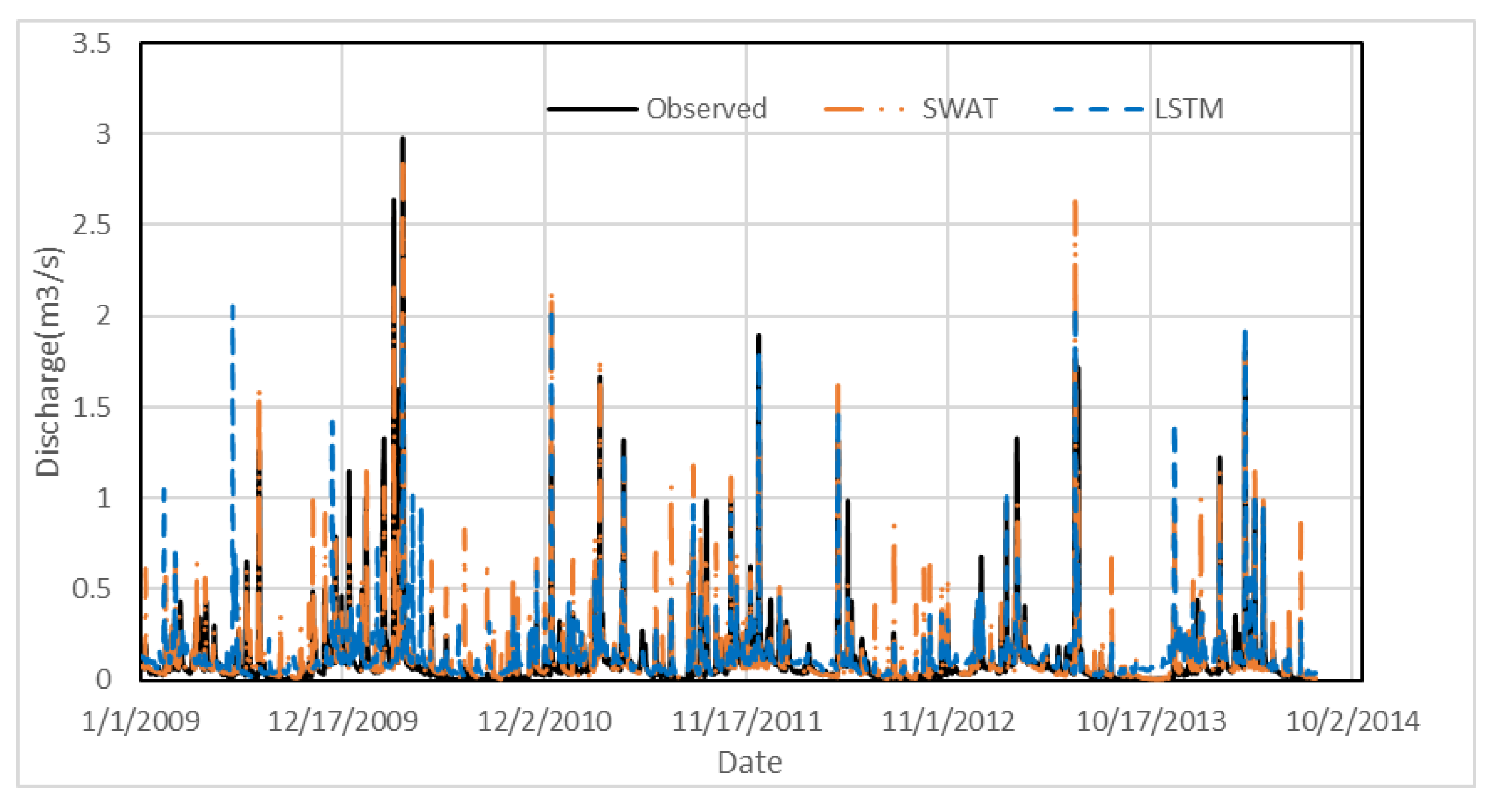
Although, modeling efforts with both conceptual and data-driven models are difficult for small watersheds, in this study, both SWAT and LSTM model results were judged satisfactorily but even though supervised calibration can be performed in SWAT, the LSTM results were comparable to SWAT results (Figure 5, Table 3). Both SWAT and LSTM results were often overestimating the low flows and some instances of high flows but did not largely overestimate peak flow as the SWAT model. The SWAT also completely misses some peaks (Figure 5) although, the physical parameters were available in SWAT with the ability to be tuned to match high flows and has been also confirmed in other studies as well [14,15,22]. In other percentiles, both models show better agreement with the observed data.
In addition to the comparison of goodness of fit, FDC and signature indices were also analyzed for a better comparison of model performance at the percentile of flows (Figure 6). From the FDC comparison at low flow areas, the difference is very apparent, but the log scale does vertical exaggeration in terms of scale. A better representation is provided by Bias FLV values. This value is positive for both SWAT and LSTM results and shows that LSTM overestimated low flows more than SWAT. As for the comparison of high flows, Bias FHV values are positive for SWAT and negative for LSTM which shows that while SWAT overestimates the peak values, LSTM underestimates it. A further look at the area under the curve till lower values of percentile from 5, 10, and 20 shows that SWAT continuously overestimates peak till 10 percentiles but starts underestimating at 20 (Table 4). In the case of LSTM, the negative discrepancy at high values continues to decrease and become positive from the 10 percentiles. The bias in low flows is very high compared to high flows and this is true for both the models. It has also been identified as LSTM’s weakness in simulating low flow.

4. Discussion

Several studies have suggested that LSTM rainfall-runoff models learn a generalizable representation of the underlying physical processes. This allows them to perform well in out-of-sample conditions, such as prediction in ungauged basins [4,19,35] and unseen extreme events [16]. These results suggest that LSTMs have captured information that generalizes to these conditions, information that can help us improve hydrological theory and predictions.
A robust hydrological model for ungauged catchment has been a challenge. SWAT has been very successful in the simulation of water quantity and quality in both gauged and ungauged watersheds across the world [57,58]. LSTM has also shown great promise in simulating flows at ungauged watersheds. Recent studies conducted with LSTM show that the prediction used in ungauged watersheds was better than conventional hydrologic models [35,58].
Interpretability and explainability in hydrological systems have always been integral to hydrological modeling [14]. Although efforts are being made for the hydrological interpretation of the LSTM from the cell states, this field is still evolving [33]. Like conceptual hydrological models, the LSTM processes the input data in increasing timestep. In every time step, LSTM internal cell states are updated from the data, which is like what a hydrological model does when it updates its states like soil moisture, snow accumulation, groundwater storage, etc. Studies have shown that individual LSTM cells correlate with snow water content, although the model was only trained to predict discharge from meteorological inputs [14]. The learned embedding of catchment attributes shows that an LSTM variant had learned to group the rainfall-runoff behaviors of hydrologically similar catchment characteristics [4]. One of the main uses of hydrological models is to understand the hydrologic response of a system under various scenarios of land use and climate change [59]. Studies show that SWAT has the ability to simulate land use changes and land use is embedded in its structure, and it could be coupled with other tools for such purposes [60,61]. There is very little research that shows the ability of LSTM to simulate under changing land use scenarios. Such research uses a modified LSTM structure called entity aware LSTM which is capable of incorporating static catchment attributed [4,62]. This may be a future direction for rainfall-runoff modeling studies.
The difficulty in hydrological modeling in smaller watersheds is large and challenging. This may be attributed to complex hydro-geological settings and nonlinear interactions among them [63]. Despite such complexities, the applicability of LSTM in small watersheds can be justified with a study with its performance metrics comparable to SWAT. This may be further tested in other smaller watersheds to bolster these results and findings. Also, it may be tested for the applicability of LSTM under land use and climate change scenarios.
However, hydrological modeling in SWAT and LSTM is not without challenges and limitations. The lack of interpretability and explainability in LSTM is present and in SWAT, this remains its core strength. On the other hand, the need for strong hydrological knowledge, and spatial data may be a major constraint for physically based models like SWAT but not a constraint for LSTM. Like other data-driven methods, LSTM networks require a large volume of data for training, which can be challenging to obtain, especially in cases where data are scarce or expensive to collect. Training LSTM networks can be computationally expensive, especially when dealing with large data and complex network architectures [64]. Due to many parameters, LSTM networks are susceptible to overfitting, especially when dealing with noisy or heterogeneous datasets hence, data validation and sufficient data are a major pivot [23]. Despite its strong architecture, LSTM can still find it difficult to establish long-term relationships, and the major hurdle when subjecting the model to data it has yet to be trained [62].

5. Conclusions

This study assessed LSTM networks for river flow simulations in small, forested watersheds, and cork brook river basins, and their prediction performances were compared against SWAT. The results from LSTM are comparable to SWAT based on goodness of fit parameters and FDC signature indices. Despite the positive results from the goodness of fit parameters, both SWAT and LSTM struggle largely at low-value estimation. Although discrepancy is also observed in high values, this is not a large discrepancy. This can be also explained as an effect of the non-linear threshold behavior of watershed [22]. Despite the successful implementation of LSTM on a small watershed, the method is scalable and applicable to larger watersheds as well. Also, to further improve the model against FDC signature indices, changes in the architecture of LSTM may be required. This could also be enhanced by the addition of static input data of DEM, Land use, and soil or some physically informed ML architecture [4].
The benefits of LSTM network models lie in their lower computational cost, lesser data need requirement, knowledge-based assessment of watersheds compared to physically based models, and its ability to handle data without requiring an in-depth understanding of the underlying physical laws. Moreover, it is superior to traditional ANN networks, which need help learning long-term dependencies such as snow accumulation, soil moisture, and groundwater storage effects crucial to the hydrological process.
LSTM models have limitations, complexity, and interpretability issues. Data availability, computation cost, model calibration and susceptibility to overfitting, difficulties in establishing long-term relationships, agnostic to data range outside training data, and interpretability are the major areas of challenge and limitation for LSTM. The lack of physical understanding of processes is a major challenge in the field of data-driven models as a whole. It hinders their ability to provide insight into the causal relationships between different hydrological variables when required. However, more research may help better understand which conceptual structures the LSTM has learned and help diagnose potential gaps existing in the current state.

Author Contributions

Conceptualization, writing—original draft preparation, S.G.S.; review and editing, S.M.P.; funding acquisition, S.M.P. All authors have read and agreed to the published version of the manuscript.

Funding

This work was supported mainly by Rhode Island Department of Planning CDBG AWD05913 and supplemted by USDA RI0014-S1063, RI0021-S1089, and McIntire Stennis RI0020-MS984.

Data Availability Statement

The data presented in this study are available upon request from the corresponding author.

Conflicts of Interest

The authors declare no conflict of interest.

References

  1. Beven, K.; Lamb, R.; Quinn, P.; Romanowicz, R.; Freer, J. Topmodel. Comput. Models Watershed Hydrol. 1995, 627–668. [Google Scholar]
  2. Kirchner, J.W. Getting the right answers for the right reasons: Linking measurements, analyses, and models to advance the science of hydrology. Water Resour. Res. 2006, 42. [Google Scholar] [CrossRef]
  3. Kollet, S.J.; Maxwell, R.M.; Woodward, C.S.; Smith, S.; Vanderborght, J.; Vereecken, H.; Simmer, C. Proof of concept of regional scale hydrologic simulations at hydrologic resolution utilizing massively parallel computer resources. Water Resour. Res. 2010, 46. [Google Scholar] [CrossRef]
  4. Kratzert, F.; Klotz, D.; Shalev, G.; Klambauer, G.; Hochreiter, S.; Nearing, G. Benchmarking a catchment-aware long short-term memory network (LSTM) for large-scale hydrological modeling. Hydrol. Earth Syst. Sci. Discuss 2019, 2019, 1–32. [Google Scholar]
  5. Wood, E.F.; Roundy, J.K.; Troy, T.J.; Van Beek, L.P.H.; Bierkens, M.F.; Blyth, E.; Whitehead, P. Hyperresolution global land surface modeling: Meeting a grand challenge for monitoring Earth’s terrestrial water. Water Resour. Res. 2011, 47. [Google Scholar] [CrossRef]
  6. Adams, T.E.; Pagano, T.C. Flood Forecasting: A Global Perspective; Academic Press: Cambridge, MA, USA, 2016. [Google Scholar]
  7. Herrnegger, M.; Senoner, T.; Nachtnebel, H.-P. Adjustment of spatio-temporal precipitation patterns in a high Alpine environment. J. Hydrol. 2018, 556, 913–921. [Google Scholar] [CrossRef]
  8. Wesemann, J.; Herrnegger, M.; Schulz, K. Hydrological modelling in the anthroposphere: Predicting local runoff in a heavily modified high-alpine catchment. J. Mt. Sci. 2018, 15, 921–938. [Google Scholar] [CrossRef]
  9. Razavi, S. Deep learning, explained: Fundamentals, explainability, and bridgeability to process-based modelling. Environ. Model. Softw. 2021, 144, 105159. [Google Scholar] [CrossRef]
  10. Remesan, R.; Mathew, J. Hydrological Data Driven Modelling; Springer: Berlin/Heidelberg, Germany, 2016. [Google Scholar]
  11. Solomatine, D.; See, L.M.; Abrahart, R.J. Data-driven modelling: Concepts, approaches and experiences. Pract. Hydroinform. Comput. Intell. Technol. Dev. Water Appl. 2008, 68, 17–30. [Google Scholar]
  12. Halff, A.H.; Halff, H.M.; Azmoodeh, M. Predicting runoff from rainfall using neural networks. In Proceedings of the Engineering Hydrology, ASCE, San Francisco, CA, USA, 25–30 July 1993. [Google Scholar]
  13. Kumar, D.N.; Raju, K.S.; Sathish, T. River flow forecasting using recurrent neural networks. Water Resour. Manag. 2004, 18, 143–161. [Google Scholar] [CrossRef]
  14. Kratzert, F.; Klotz, D.; Brenner, C.; Schulz, K.; Herrnegger, M. Rainfall–runoff modelling using long short-term memory (LSTM) networks. Hydrol. Earth Syst. Sci. 2018, 22, 6005–6022. [Google Scholar] [CrossRef]
  15. Lees, T.; Buechel, M.; Anderson, B.; Slater, L.; Reece, S.; Coxon, G.; Dadson, S.J. Benchmarking data-driven rainfall–runoff models in Great Britain: A comparison of long short-term memory (LSTM)-based models with four lumped conceptual models. Hydrol. Earth Syst. Sci. 2021, 25, 5517–5534. [Google Scholar] [CrossRef]
  16. Frame, J.M.; Kratzert, F.; Klotz, D.; Gauch, M.; Shalev, G.; Gilon, O.; Qualls, L.M.; Gupta, H.V.; Nearing, G.S. Deep learning rainfall–runoff predictions of extreme events. Hydrol. Earth Syst. Sci. 2022, 26, 3377–3392. [Google Scholar] [CrossRef]
  17. Schmidhuber, J.; Hochreiter, S. Long short-term memory. Neural Comput. 1997, 9, 1735–1780. [Google Scholar]
  18. Saha, G.K.; Rahmani, F.; Shen, C.; Li, L.; Cibin, R. A deep learning-based novel approach to generate continuous daily stream nitrate concentration for nitrate data-sparse watersheds. Sci. Total. Environ. 2023, 878, 162930. [Google Scholar] [CrossRef] [PubMed]
  19. Ma, K.; Feng, D.; Lawson, K.; Tsai, W.P.; Liang, C.; Huang, X.; Shen, C. Transferring hydrologic data across continents–leveraging data-rich regions to improve hydrologic prediction in data-sparse regions. Water Resour. Res. 2021, 57, e2020WR028600. [Google Scholar] [CrossRef]
  20. Yang, T.; Sun, F.; Gentine, P.; Liu, W.; Wang, H.; Yin, J.; Du, M.; Liu, C. Evaluation and machine learning improvement of global hydrological model-based flood simulations. Environ. Res. Lett. 2019, 14, 114027. [Google Scholar] [CrossRef]
  21. Tao, Y.; Gao, X.; Hsu, K.; Sorooshian, S.; Ihler, A. A deep neural network modeling framework to reduce bias in satellite precipitation products. J. Hydrometeorol. 2016, 17, 931–945. [Google Scholar] [CrossRef]
  22. Ley, A.; Bormann, H.; Casper, M. Intercomparing LSTM and RNN to a Conceptual Hydrological Model for a Low-Land River with a Focus on the Flow Duration Curve. Water 2023, 15, 505. [Google Scholar] [CrossRef]
  23. Nifa, K.; Boudhar, A.; Ouatiki, H.; Elyoussfi, H.; Bargam, B.; Chehbouni, A. Deep Learning Approach with LSTM for Daily Streamflow Prediction in a Semi-Arid Area: A Case Study of Oum Er-Rbia River Basin, Morocco. Water 2023, 15, 262. [Google Scholar] [CrossRef]
  24. Hu, C.; Wu, Q.; Li, H.; Jian, S.; Li, N.; Lou, Z. Deep learning with a long short-term memory networks approach for rainfall-runoff simulation. Water 2018, 10, 1543. [Google Scholar] [CrossRef]
  25. Sungmin, O.; Dutra, E.; Orth, R. Robustness of process-based versus data-driven modeling in changing climatic conditions. J. Hydrometeorol. 2020, 21, 1929–1944. [Google Scholar]
  26. Hunt, K.M.R.; Matthews, G.R.; Pappenberger, F.; Prudhomme, C. Using a long short-term memory (LSTM) neural network to boost river streamflow forecasts over the western United States. Hydrol. Earth Syst. Sci. 2022, 26, 5449–5472. [Google Scholar] [CrossRef]
  27. Barzegar, R.; Aalami, M.T.; Adamowski, J. Short-term water quality variable prediction using a hybrid CNN–LSTM deep learning model. Stoch. Environ. Res. Risk Assess. 2020, 34, 415–433. [Google Scholar] [CrossRef]
  28. Hettiarachchi, P.; Hall, M.J.; Minns, A.W. The extrapolation of artificial neural networks for the modelling of rainfall—Runoff relationships. J. Hydroinformatics 2005, 7, 291–296. [Google Scholar] [CrossRef]
  29. Noori, N.; Kalin, L.; Isik, S. Water quality prediction using SWAT-ANN coupled approach. J. Hydrol. 2020, 590, 125220. [Google Scholar] [CrossRef]
  30. Pascanu, R.; Mikolov, T.; Bengio, Y. On the difficulty of training recurrent neural networks. In Proceedings of the International Conference on Machine Learning, Pmlr, Atlanta, GA, USA, 16–21 June 2013. [Google Scholar]
  31. Schmidhuber, J. Deep learning in neural networks: An overview. Neural Netw. 2015, 61, 85–117. [Google Scholar] [CrossRef]
  32. Essam, Y.; Huang, Y.F.; Ng, J.L.; Birima, A.H.; Ahmed, A.N.; El-Shafie, A. Predicting streamflow in Peninsular Malaysia using support vector machine and deep learning algorithms. Sci. Rep. 2022, 12, 383. [Google Scholar] [CrossRef]
  33. Klotz, D.; Kratzert, F.; Gauch, M.; Sampson, A.K.; Brandstetter, J.; Klambauer, G.; Hochreiter, S.; Nearing, G. Uncertainty estimation with deep learning for rainfall–runoff modeling. Hydrol. Earth Syst. Sci. 2022, 26, 1673–1693. [Google Scholar] [CrossRef]
  34. Liang, W.; Chen, Y.; Fang, G.; Kaldybayev, A. Machine learning method is an alternative for the hydrological model in an alpine catchment in the Tianshan region, Central Asia. J. Hydrol. Reg. Stud. 2023, 49, 101492. [Google Scholar] [CrossRef]
  35. Feng, D.; Beck, H.E.; Lawson, K.; Shen, C. The suitability of differentiable, physics-informed machine learninghydrologic models for ungauged regions and climate change impact assessment. Hydrol. Earth Syst. Sci. 2023, 17, 2357–2373. [Google Scholar] [CrossRef]
  36. Merz, R.; Blöschl, G.; Parajka, J. Spatio-temporal variability of event runoff coefficients. J. Hydrol. 2006, 331, 591–604. [Google Scholar] [CrossRef]
  37. Moriasi, D.N.; Arnold, J.G.; van Liew, M.W.; Bingner, R.L.; Harmel, R.D.; Veith, T.L. Model evaluation guidelines for systematic quantification of accuracy in watershed simulations. Trans. ASABE 2007, 50, 885–900. [Google Scholar] [CrossRef]
  38. Homer, C.; Dewitz, J.; Yang, L.; Jin, S.; Danielson, P.; Xian, G.; Megown, K. Completion of the 2011 National Land Cover Database for the conterminous United States–representing a decade of land cover change information. Photogramm. Eng. Remote Sens. 2015, 81, 345–354. [Google Scholar]
  39. Addy, K.; Gold, A.J.; Loffredo, J.A.; Schroth, A.W.; Inamdar, S.P.; Bowden, W.B.; Kellogg, D.Q.; Birgand, F. Stream response to an extreme drought-induced defoliation event. Biogeochemistry 2018, 140, 199–215. [Google Scholar] [CrossRef]
  40. Krysanova, V.; Arnold, J.G. Advances in ecohydrological modelling with SWAT—A review. Hydrol. Sci. J. 2008, 53, 939–947. [Google Scholar] [CrossRef]
  41. Walega, A.; Amatya, D.M.; Caldwell, P.; Marion, D.; Panda, S. Assessment of storm direct runoff and peak flow rates using improved SCS-CN models for selected forested watersheds in the Southeastern United States. J. Hydrol. Reg. Stud. 2020, 27, 100645. [Google Scholar] [CrossRef]
  42. Marin, M.; Clinciu, I.; Tudose, N.C.; Ungurean, C.; Adorjani, A.; Mihalache, A.L.; Davidescu, A.A.; Davidescu, O.; Dinca, L.; Cacovean, H. Assessing the vulnerability of water resources in the context of climate changes in a small forested watershed using SWAT: A review. Environ. Res. 2020, 184, 109330. [Google Scholar] [CrossRef] [PubMed]
  43. Im, S.; Lee, J.; Kuraji, K.; Lai, Y.-J.; Tuankrua, V.; Tanaka, N.; Gomyo, M.; Inoue, H.; Tseng, C.-W. Soil conservation service curve number determination for forest cover using rainfall and runoff data in experimental forests. J. For. Res. 2020, 25, 204–213. [Google Scholar] [CrossRef]
  44. Abbaspour, K.C.; Rouholahnejad, E.; Vaghefi, S.; Srinivasan, R.; Yang, H.; Kløve, B. A continental-scale hydrology and water quality model for Europe: Calibration and uncertainty of a high-resolution large-scale SWAT model. J. Hydrol. 2015, 524, 733–752. [Google Scholar] [CrossRef]
  45. Siami-Namini, S.; Tavakoli, N.; Namin, A.S. The performance of LSTM and BiLSTM in forecasting time series. In Proceedings of the 2019 IEEE International Conference on Big Data (Big Data), Los Angeles, CA, USA, 9–12 December 2019. [Google Scholar]
  46. Alizadeh, B.; Bafti, A.G.; Kamangir, H.; Zhang, Y.; Wright, D.B.; Franz, K.J. A novel attention-based LSTM cell post-processor coupled with bayesian optimization for streamflow prediction. J. Hydrol. 2021, 601, 126526. [Google Scholar] [CrossRef]
  47. Man, Y.; Yang, Q.; Shao, J.; Wang, G.; Bai, L.; Xue, Y. Enhanced LSTM model for daily runoff prediction in the upper huai river basin, China. Engineering 2022, 24, 229–238. [Google Scholar] [CrossRef]
  48. Zulqarnain, M.; Ghazali, R.; Hassim, Y.M.M.; Aamir, M. An Enhanced gated recurrent unit with auto-encoder for solving text classification problems. Arab. J. Sci. Eng. 2021, 46, 8953–8967. [Google Scholar] [CrossRef]
  49. Joseph, V.R. Optimal ratio for data splitting. Stat. Anal. Data Min. ASA Data Sci. J. 2022, 15, 531–538. [Google Scholar] [CrossRef]
  50. Arnold, J.G.; Moriasi, D.N.; Gassman, P.W.; Abbaspour, K.C.; White, M.J.; Srinivasan, R.; Jha, M.K. SWAT: Model use, calibration, and validation. Trans. ASABE 2012, 55, 1491–1508. [Google Scholar] [CrossRef]
  51. Yilmaz, K.K.; Gupta, H.V.; Wagener, T. A process-based diagnostic approach to model evaluation: Application to the NWS distributed hydrologic model. Water Resour. Res. 2008, 44, 1–18. [Google Scholar] [CrossRef]
  52. Chambers, B.M.; Pradhanang, S.M.; Gold, A.J. Simulating Climate change induced thermal stress in coldwater fish habitat using SWAT model. Water 2017, 9, 732. [Google Scholar] [CrossRef]
  53. Gupta, A.; Govindaraju, R. Propagation of structural uncertainty in watershed hydrologic models. J. Hydrol. 2019, 575, 66–81. [Google Scholar] [CrossRef]
  54. Moges, E.; Demissie, Y.; Larsen, L.; Yassin, F. Review: Sources of hydrological model uncertainties and advances in their analysis. Water 2020, 13, 28. [Google Scholar] [CrossRef]
  55. Li, H.; Sivapalan, M. Effect of spatial heterogeneity of runoff generation mechanisms on the scaling behavior of event runoff responses in a natural river basin. Water Resour. Res. 2011, 47. [Google Scholar] [CrossRef]
  56. Brantley, S.L.; Lebedeva, M.I.; Balashov, V.N.; Singha, K.; Sullivan, P.L.; Stinchcomb, G. Toward a conceptual model relating chemical reaction fronts to water flow paths in hills. Geomorphology 2017, 277, 100–117. [Google Scholar] [CrossRef]
  57. Rempe, D.M.; Dietrich, W.E. A bottom-up control on fresh-bedrock topography under landscapes. Proc. Natl. Acad. Sci. USA 2014, 111, 6576–6581. [Google Scholar] [CrossRef]
  58. Kratzert, F.; Klotz, D.; Herrnegger, M.; Sampson, A.K.; Hochreiter, S.; Nearing, G.S. Toward Improved predictions in ungauged basins: Exploiting the power of machine learning. Water Resour. Res. 2019, 55, 11344–11354. [Google Scholar] [CrossRef]
  59. Lin, Y.-P.; Hong, N.-M.; Wu, P.-J.; Lin, C.-J. Modeling and assessing land-use and hydrological processes to future land-use and climate change scenarios in watershed land-use planning. Environ. Geol. 2007, 53, 623–634. [Google Scholar] [CrossRef]
  60. Guo, W.; Yu, L.; Huang, L.; He, N.; Chen, W.; Hong, F.; Wang, B.; Wang, H. Ecohydrological response to multi-model land use change at watershed scale. J. Hydrol. Reg. Stud. 2023, 49, 101517. [Google Scholar] [CrossRef]
  61. Dixon, B.; Earls, J. Effects of urbanization on streamflow using SWAT with real and simulated meteorological data. Appl. Geogr. 2012, 35, 174–190. [Google Scholar] [CrossRef]
  62. Bai, P.; Liu, X.; Xie, J. Simulating runoff under changing climatic conditions: A comparison of the long short-term memory network with two conceptual hydrologic models. J. Hydrol. 2021, 592, 125779. [Google Scholar] [CrossRef]
  63. Yan, L.; Chen, C.; Hang, T.; Hu, Y. A stream prediction model based on attention-LSTM. Earth Sci. Inform. 2021, 14, 723–733. [Google Scholar] [CrossRef]
  64. Lipton, Z.C.; Berkowitz, J.; Elkan, C. A critical review of recurrent neural networks for sequence learning. arxiv 2015, arXiv:1506.00019. [Google Scholar]
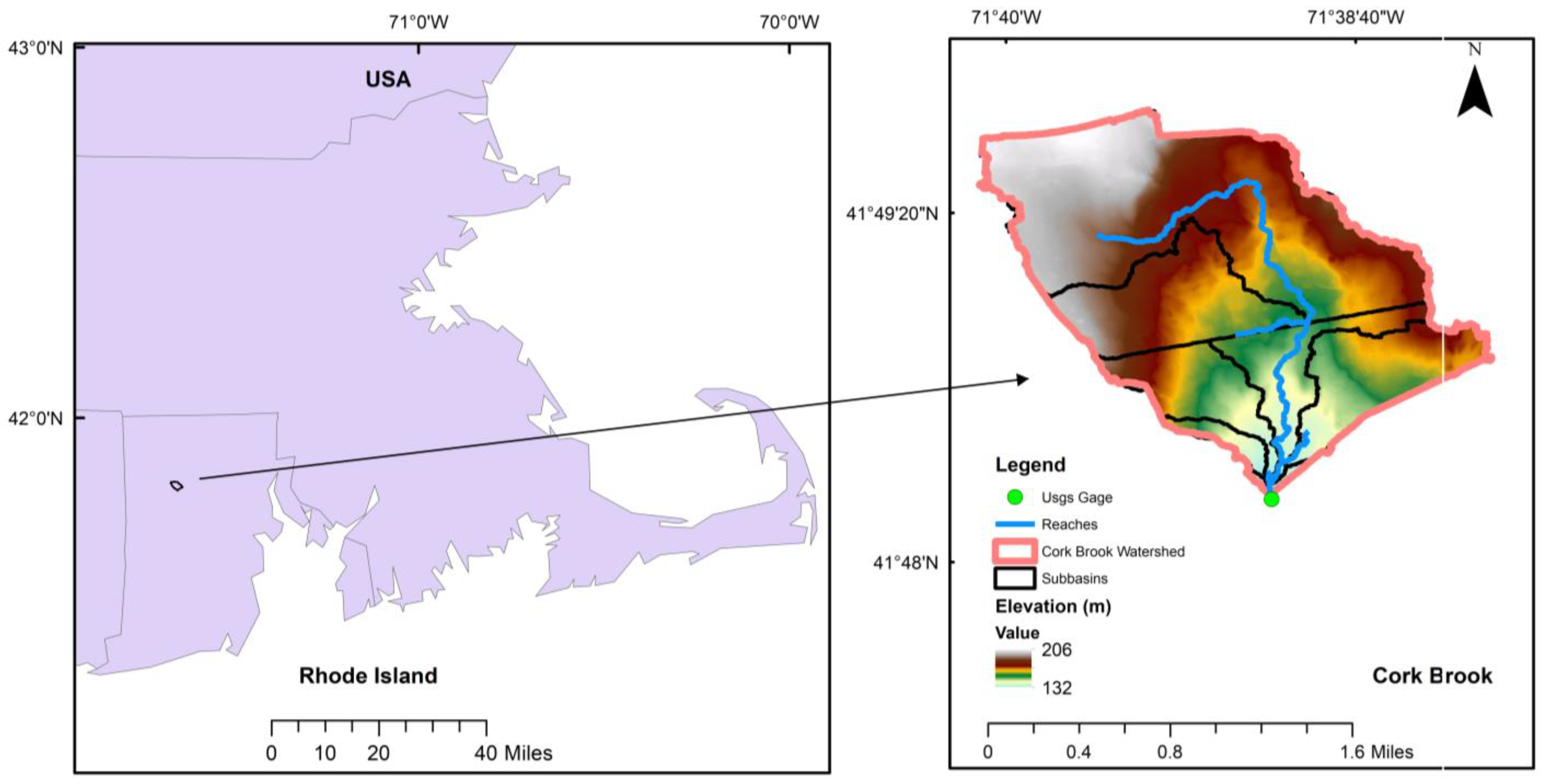
Figure 1. Study Area: and Elevation variation in Cork Brook Watershed, Rhode Island, USA.
Water 15 04194 g001
Figure 2. Land use and Soil Distribution in Cork Brook.
Water 15 04194 g002
Figure 3. Daily Hydrometeorological data in Cork Brook, RI (a) Discharge (b) Precipitation (c) Temperature.
Water 15 04194 g003
Figure 4. The structure of the LSTM model. The subscript “t” here represents the current time and represents the hidden state and cell state [48].
Water 15 04194 g004
Figure 5. Simulated vs Observed flow at USGS Gauge 01115280.
Water 15 04194 g005
Figure 6. Comparison of (a) Flow Duration Curve Comparison (b) Signature indices.
Water 15 04194 g006
Table 1. Range of sensitive parameters during SWAT streamflow calibration.
ParameterDefinitionRangeUnits
CN2.mgt SCS runoff curve number 60–75-
ALPHA_BF.gw Baseflow alpha factor 0.0–0.101/Days
GW_DELAY.gwGroundwater delay0.0–7.0Days
GWQMN.gwDepth of water in shallow aquifer for return flow0–1000 mmmm
SMTMP.bsn Snowmelt base temperature−0.5–2.0°C
ESCO.hru Soil evaporation compensation factor 0.15–0.65 -0.15–0.65-
ALPHA_BNKBaseflow alpha factor for bank storage0.0–7.0Days
SLSOIL.hru Slope length for lateral subsurface flow 0.0–15m
Table 2. Model Structure and parameters for LSTM streamflow calibration.
Layer (Type)Output ShapeParam #
Lstm_1 (LSTM)(None, 10, 75)23,400
Dropout_1 (Dropout)(None, 10, 75)0
Lstm_2 (LSTM)(None, 10, 75)45,300
Dropout_2 (Dropout)(None, 10, 75)0
Lstm_3 (LSTM)(None, 10, 75)45,300
Dropout_3 (Dropout)(None, 10, 75)0
Lstm_4 (LSTM)(None, 10, 75)45,300
Dropout_4 (Dropout)(None, 10, 75)0
Lstm_5 (LSTM)(None, 75)45,300
Dense_1 (Dense)(None, 75)5700
Dense_2 (Dense)(None, 1)76
Total Params: 210376
Table 3. Goodness of fit Parameters.
Calibration (2009–2013)Validation (2013–2014)
SWATLSTMSWATLSTM
NSE0.650.770.630.60
R20.680.780.680.65
Table 4. Deviation of SWAT and LSTM FDC from Observed FDC.
Deviation (%)
PercentileSWATLSTM
25−7
54−3
1001
20−97
Disclaimer/Publisher’s Note: The statements, opinions and data contained in all publications are solely those of the individual author(s) and contributor(s) and not of MDPI and/or the editor(s). MDPI and/or the editor(s) disclaim responsibility for any injury to people or property resulting from any ideas, methods, instructions or products referred to in the content.