1. Introduction
Hydraulic fracturing (HF) is considered a vital method for advancing petroleum, whether in conventional or unconventional natural gas [
1,
2,
3]. A surplus of fluid is expelled, surpassing what poroelasticity can withstand, aiming to stimulate hydraulic volumetric openings in reservoir formations. Consequently, permeability is enhanced [
4,
5,
6]. However, in return, this volumetric opening will stimulate the manifestation of an additional confining stress on the material skeleton, which is called the confining stress response [
7,
8,
9]. Since micro- or nano-pores in the skeleton matrix are the main sorption space for unconventional gas, confining stress response will inevitably reduce the matrix permeability and hamper gas production [
10,
11,
12]. Therefore, it is necessary to evaluate the confining stress response during the implementation of an HF.
The confining stress response due to HF treatment was first noted by Cleary [
13]. This effect was called far-field confining stress and described as back stress, namely
, which was different from confining stress. The author also reported that back stress arises from the alteration of the pore pressure due to fluid infiltration into the surrounding rocks. Since Detournay and Cheng [
14] associated back stress with Biot’s theory of poroelasticity, various types of poroelastic effects have been reported in the literature.
On top of that, Detournay and Cheng [
15] included poroelastic effects in the PKN model by setting up a constitutive relationship between the fluid pressure and width of fracture with the poroelastic coefficient. Kovalyshen [
16] associated poroelastic effects with a radial model by establishing a boundary integral form of back stress.
On another front, studies on the poroelastic effects based on the application of direct numeric methods can be classified into two branches, namely, single-fracture models and multiple-fracture models.
In the first branch, Boone and Ingraffea [
17] studied the poroelastic effect by carrying out Finite Element Method (FEM) simulations and demonstrated that the back stress was the minimum at the borehole and maximum at the fracture tip. In another interesting work, Golovin and Baykin [
18] demonstrated the influence of Biot’s number on pore pressure and fracture width distributions. Gao and Detournay [
19] investigated two fracture regimes in laboratory hydraulic fracturing and concluded that poroelasticity can significantly affect the magnitude of the injection pressure. Baykin [
20] proved that the diffusion scale plays a central role in the poroelastic effects, while Donstsov [
21] developed an efficient computation method of poroelastic stress, which is a combination of the one-dimensional Carter leak-off model and back stress. Moreover, Sarris and Papanastasiou [
22,
23,
24] studied the poroelasto-plastic effects and showed that a rabbit-ear-shaped plastic zone was developed near the fracture tip, and demonstrated that the poroelasto-plastic effect was responsible for larger net pressure and fracture width.
In another branch, multiple fracturing modeling was performed to demonstrate stress shadow and fracturing interference based on the utilization of various numeric methods, like the PFC model [
25], XFEM [
26,
27], Abaqus model [
28], DNF model [
29,
30], phase field model [
31], UDEC [
10], the lattice model [
32], etc. Particularly, Dontsov and Suarez-Rivera [
33] found that the propagation of multiple closely spaced hydraulic fractures varies dramatically with respect to the fracture propagation regimes.
To sum up, previous studies on the poroelastic effect have mainly focused on the global fracture scale, whereas the conclusions are significantly dependent on the fracture geometry and other engineering factors. However, from the HF evaluation perspective, it is necessary to establish a stress disturbance evaluation model, namely, a representative volume element (RVE) evaluation model. The RVE model can integrate the macro attributes of the reservoir and injected fluid, such as elasticity, toughness, leakage, permeability, flow rate, viscosity, and compressibility, and then, the coupling and matching relationship between the reservoir cohesive fracture characteristics and fracture propagation mechanism can be characterized.
In this work, an RVE evaluation model of confining stress response was established based on the hydraulic volumetric opening (HVO) model. The HVO model, proposed by Wang et al. [
34], is a combination of the poroelasticity, breakdown damage, and hydraulic fracture mechanics theories. The pore volumetric opening and fracture volumetric opening were unified in an RVE by matching the behaviors of the channel flow in a KGD fracture, the porous elastic opening, and the cohesive breakdown. Based on the HVO model, the confining stress response model was established by utilizing the deformation compatibility during the hydraulic fracturing opening. Finally, as an example, under the four limiting hydraulic fracturing regimes, the evolution law of stress disturbance was exhibited based on the HVO model.
2. The Model of Confining Stress Response to the HVO
2.1. Staged Expressions of the HVO
Considering an RVE in the hydraulic fracturing region, as is shown in
Figure 1, the original state of the material was isotropic, homogeneous, perfectly elastic, and permeated with void spaces of various shapes and sizes, such as microcracks, fissures, and pores, all of which were idealized as pore volume. Since the fluid injection (represented by
) and pore volume are saturated and the pore pressure is built up, this effect, in turn, leads to the pore volume being elastically opened, the matrix skeleton being elastically stretched and broken, and eventually, the formation of a trunk fracture from the chained skeletons’ breakdown. According to the increase in the skeleton stress, this process can be segmented into three distinct stages, characterized by four typical states:
Stage I, which can be described as the compression-relieving stage, involves the original compressive stress on the skeletons being gradually balanced to zero by the pore pressure. In Stage II, this stage can be described as an elastic stretching phase, during which the matrix skeleton undergoes stretching due to the opening of the pore volume. In Stage III, which is a cohesive breakdown stage, the chained cohesive breakdown occurs, the trunk fracture takes its form, and fracture opening occurs.
Correspondingly, the four typical states are the following: ‘A’ is the original compression state under the confining stress; ‘B’ represents the stress neutralization state, wherein the skeleton stress becomes zero as the pore pressure balances the confining stress. ‘C’ is the critical state, where the elastically stretching microcracking approaches the end and the macro-breakdown is about to happen, and ‘D’ is the fracture opening that approaches a steady state.
For this tip process, three hydraulic volumetric openings can be defined:
The pore volumetric opening,
, is defined as the volumetric opening of pores per unit bulk volume of rocks. In terms of quantity, it represents the increment in the elastic net volume of void spaces of various shapes and sizes due to the influence of pore fluid pressure. The fracture volumetric opening,
, is defined as the trunk fracture volumetric opening per unit bulk volume of the rocks. For a plane strain fracturing and cubic element of a unit bulk volume,
, where
is the fracture width. The hydraulic volumetric opening,
, is the total volumetric opening per unit bulk volume of rocks. Quantitatively, it signifies the net increment in porosity resulting from hydraulic fracturing. The progressive development of these volumetric openings can be described as follows:
Applying the poroelasticity theory [
35], incremental expressions for volumetric openings can be found in the literature [
34], as follows
where
is the flexibility of the matrix material;
is scalar damage representing the progress of the chained breakdown with
;
stands for an evolving function, representing the evolution of the bulk modulus, compressibilities, and Biot’s coefficient due to cohesive breakdown; and
refers to the residual Biot coefficient relative to the original Biot coefficient
.
2.2. Breakdown Criterion and Evolving Laws of State Variables
The breakdown criterion is defined on a quasi-static evolving path of the skeleton stress, which is characterized by a smoothed peak and a long tail, shown by
in
Figure 2. The progress of cohesive breakdown can be represented by scalar damage as follows:
Of the parameters in Equation (3),
signifies the ultimate strain anticipated for a flawless brittle fracture,
indicates the transition strain from the evolution of microcracks to the propagation of macrocracks,
denotes the brittle index,
represents residual stress,
is the ratio of the stress drop at
reflecting the intensity of the stress drop, and
is the stress drop from the initiation of macrocrack propagation to the residual stress. All these parameters can be determined from the uniaxial tensile stress–strain curve, as illustrated in
Figure 2.
Ensuring a mathematically smooth connection at
requires the construction of the two parameters
and
from other measured parametric groups
, as follows:
Thus, it can be seen that the breakdown behavior is stipulated by the parametric group under anhydrous conditions, except for the basic Young modulus .
The comparative advantage of the smoothed-peak stress curve over the sharp-peak models, such as the classic cohesive zone model [
36] and the exponential softening model [
22], is that the microcracking process prior to the large-scale breakdown can be reflected. Additionally, the advantage of the long tail is that a continuous function is used to represent the gradual fracture opening, which, in fact, prolongs the tip process to the whole of the fracture.
2.3. Model of Confining Stress Response on RVE
In order to establish the confining stress response model of the fluid injection around the fracture during the process of hydraulic fracturing, the RVE element of the reservoir was selected in the steady flow state during the fracturing process (
Figure 3a), and the schematic diagram of its plane stress model (
Figure 3b) was constructed. The total in situ confining stress is the sum of the back stress and the far-field stress, namely
.
As can be observed from
Figure 3b, the bulk volume expansion induced by the hydraulic volumetric opening is constrained by the combination of the pore pressure and additional confining stress. In the direction of the fracture opening, it was assumed that the pore pressure
and fracture pressure
are equal; thus,
. Therefore, combined with the principle of mechanical equilibrium and deformation compatibility, this constraint can be described by using the compatibility relation as follows:
where
is the bulk volume expansion due to pore pressure,
represents the bulk volume compression due to back stress, and
denotes the total bulk volume expansion due to the hydraulic volumetric opening.
From Equation (2),
can be rewritten into the following expression:
where
is the portion of the volumetric opening due to the pore pressure, and
represents that due to skeleton stress. In the same way,
can be decomposed as follows:
where
is the unit bulk volume,
is the incremental bulk volume due to the fracture volume opening merely attributed to pore pressure, and
stands for the incremental bulk volume due to the pore volume opening attributed to the incremental pore pressure. It is the same with
and
.
The substitution of Equation (5) with Equation (7) yields the following expression:
where
represents the rigid expansion to be replaced by the fracture volumetric opening
;
signifies the poroelastic expansion to be translated by the ratio
of compressibilities, which was defined by Zimmerman. Thus, it can be described as follows:
By including the terms in Equation (7), and letting
and
(not that
is the initial pore volume in
here), the following equation can be derived:
The relations between those compressibilities were used by Zimmerman, and = the initial compression under confining stress
was superposed as follows:
By using the elasticity law
, the total confining stress can be obtained as follows:
By assuming
, the bulk volume expansion and confining stress are as follows:
This is the constitutive relationship between the total in situ confining stress response and the hydraulic fracturing volumetric opening. The integration was executed along the injection time or the skeleton strain , while it was demonstrated that the confining stress response was determined not only by the rock elasticity properties but also by the characteristics of cohesive breakdown and fracturing propagation regimes, which were represented by the parametric group .
3. Incorporating the Regimes of Hydraulic Fracturing Propagation
Various works in the literature [
37,
38,
39,
40] have proposed hydraulic fracturing regimes based on simple planar models, including KGD, PKN, and radial, based on the controlling equations in hydraulic fracturing. It was found that the interactions of channel flow in a planar fracture with rock elasticity, toughness, and leak-off can be categorized into four distinct limiting fracturing regimes and intermediate fracturing regimes within the parameter space that is expanded by the dimensionless viscosity
and dimensionless toughness
. Moreover, the various fracturing regimes take on varying temporal evolutions of the fracture width, length, and fluid pressure distribution.
The incorporation of fracturing regimes into the HVO model was employed to combine the channel flow of the fracturing regimes with the cohesive breakdown and volumetric opening, to obtain the proper evolution of the HVO model. From another point of view, Carter’s leak-off, addressing fluid loss from the planar fracture, governs the fracturing regimes, while Darcy’s law, which governs the volumetric openings of the pores, concerns the porous flow of the filtrated fluid. Therefore, this incorporation is indeed a unification of Carter’s leak-off model and Darcy’s law in the HVO model.
In fact, this incorporation can be realized by matching the temporal evolution of the fracture volumetric opening with the temporal evolution of a KGD fracture width to obtain the proper evaluation of the parameter group . In this operation, the KGD fracture width, denoted as , represents the fluid load in the HVO model, and the parameter group refers to the constitutive response of the cohesive breakdown and the volumetric opening of the rock.
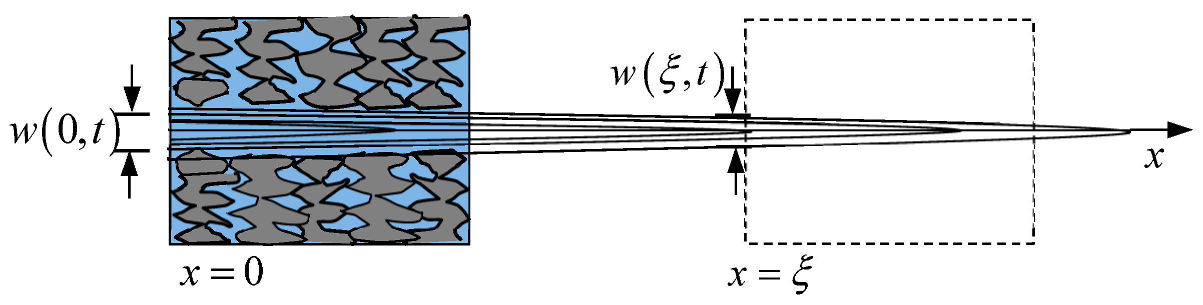
It is well established that the fracturing regimes provide fracture width distribution
along the fracture length, as is shown in
Figure 4. The problem lies with the selection of the position
. More specifically, because the HVO model plays the role of a constitutive relationship, it should be endowed with all the characteristics of the cohesive breakdown and volumetric opening for the entire hydraulic fracturing process. Obviously, only at the fracture inlet (where
), the fracture width
can satisfy this requirement, while at other positions (like
), the width evolution will undergo the same as that at the fracture inlet. However, the experience is incomplete because of the propagation delay.
Since the analytical solutions for fracture width
can be found in the article [
40], the properly evaluated parameter group
can be obtained by carrying out curve fitting between
and
.
4. Examples
Examples were used to demonstrate how to evaluate the confining stress response due to HF and the constitutive relationship between the confining stress response and HVOs in four limiting fracturing cases. These four limiting cases corresponded to the four limiting fracturing regimes; these, include the viscosity–storage-dominated regime , the viscosity–leak-off-dominated regimes , the toughness–storage regime , and the toughness–leak-off-dominated regime , respectively.
4.1. The Process for Obtaining the Parameters of the Confining Stress Response Model
The procedure followed the following sequences: parameter measurement; parameter transition; determination of the computation time; obtaining the best-fitted parameter group via curve fitting; and obtaining the evolving hydraulic volumetric opening and confining stress response.
4.1.1. Parameter Measurement
The evaluation of the confining stress response and the volumetric opening was based on the poromechanical parameters that were collected from the field. In the examples, the basic parameters for all the fracturing cases were taken from a coal bed methane (CBM) reservoir formation located in Qinshui Basin in Shanxi Province, China; a reservoir formation thickness of
, Young’s modulus of
, Poisson’s ratio of
, injection flow rate of
, viscosity of
, and fluid compressibility of
were assumed. The other parameters related to the fracturing regimes, such as tensile strength
, static confining stress
, original confining stress
, permeability
, porosity
, and Biot’s coefficient
, are listed in
Table 1.
4.1.2. Parameter Conversion
Because the fracturing regimes were derived from the KGD models, the measured parameters in
Table 2 needed to be converted into the KGD system according to the relations shown in
Table 2. In these conversions,
is the size of micro-defects in rocks, and
represents the diffusion coefficient. Based on these, the KGD parameters for fracturing regime recognition were calculated and are shown in
Table 3.
4.1.3. Computation Time
Hu and Garagash [
40] demonstrated that various fracturing regimes can be reduced to four distinct limiting and intermediate regimes in the dimensionless parametric space
or
through the following divisions:
where
represents the dimensionless toughness coefficient,
stands for the dimensionless leak-off coefficient in viscosity-dominated regimes, and
indicates the dimensionless leak-off coefficient in toughness-dominated regimes. These coefficients are defined as follows:
where
represents the injection time, and
is a characteristic time.
From these divisions, it can be argued that if these limiting fracturing regimes hold, the computation time
in the different regimes can be determined as follows:
According to these conditions, the computation times in the different regimes were determined and are listed in
Table 2. The dimensionless coefficients for regime recognition are listed in
Table 4.
4.1.4. Curve Fitting
The curve fitting between
and
was carried out to obtain the best-fitted parameter group
by adjusting the combination. The expressions for
in the four limiting regimes were drawn from [
40], as follows:
The curve-fitting process followed the steps:
(1) The injection time,
, was given to calculate the skeleton strain as follows:
where
is the limiting tensile strain corresponding to tensile strength
,
;
is a characterized time corresponding to
and can be determined through a static tensile test. However, in this work, the value of
was selected.
(2) , , and were calculated.
(3) , , and , as well as , , and , were calculated by accumulating , etc.
(4) was fitted with to obtain the group with the best combination of parameters and the number of hydraulic fractures .
(5) The change laws of , , and were obtained.
4.2. Physical Meanings of the Curve Fitting
Parametric groups
in four limiting regimes were obtained through curve fitting and are listed in
Table 4, upon which all the variables were obtained, including hydraulic volumetric openings, confining stress response, skeleton stress, pore pressure, and breakdown damage. In addition, both fracture number
and hydraulically tensile strength
were also obtained.
The curve fitting led to the fracture number and hydraulic tensile strength being less than in the anhydrous conditions, . This reflects the physical meanings of the curve fitting.
The meaning for is that, in the condition of a single fracture, will lead to a relatively large , meaning that the fracture volumetric opening cannot match up. Only when , so that and it generates a proper , can match up well. This effect implies that, for a single KGD fracture, is derived merely from the channel flow regimes without considering the constraints of the rock breakdown characteristics and overstates the fracture opening capacity. As far as the spatial distribution of these fractures is concerned, it may be parallel or branching, while all fractures followed the distribution of the pre-existing crack. In the current mechanism, the two storage-dominated regimes and were recognized to be liable for the generation of more multiple fractures than the leak-off-dominated regimes and .
The underlying reason for the hydraulic tensile strength being less than the anhydrous tensile strength is that, in the hydraulic fracturing model, the fluid goes ahead of the fracture tip both in stages I and II, and microcracking before breakdown is permitted, which induces a more liable breakdown than in the anhydrous conditions. In the current fracturing mechanisms, it was found that in the toughness-dominated regimes and was significantly lower than that in the viscosity-dominated regimes and , and that in the leak-off-dominated regimes and was less than in the storage-dominated regimes and .
All these effects reflect the physical meanings of the curve fittings, where, in an HF process, fluid injection is an active force represented by the fracture propagation regimes . Moreover, is an adaption response, which is represented by the parameter group , and the matching between them generates a number of fractures and hydraulic tensile strength .
4.3. Results and Validation
4.3.1. Hydraulic Volumetric Openings
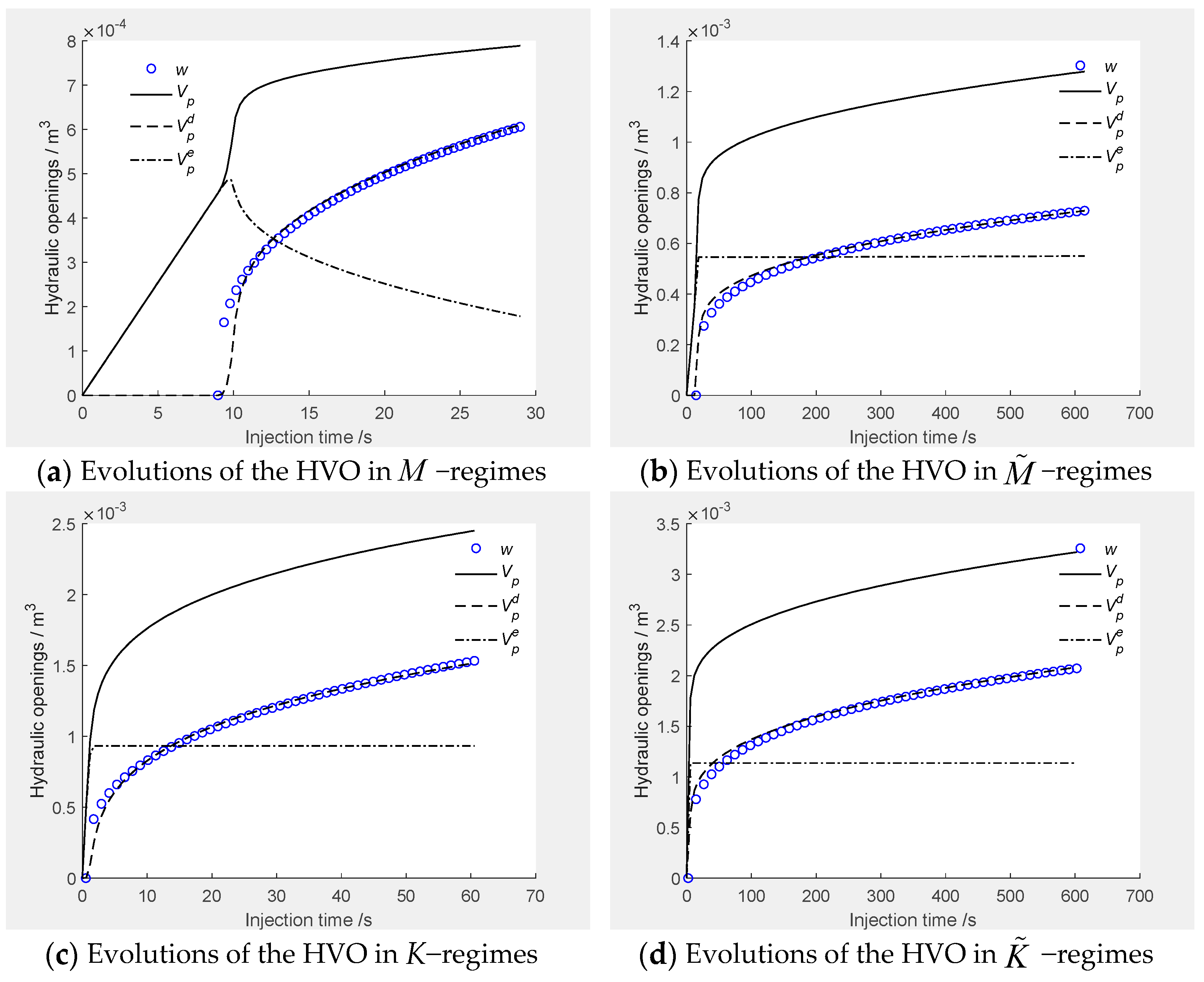
The change patterns of hydraulic volumetric openings are depicted in
Figure 5. The
first increased linearly from the compression state to a peak, followed by a decline to a low level as soon as the breakdown began. Then,
was increased following a power law. As a sum,
first increased following the pore volumetric opening, then reached a constant level as soon as the fracture volumetric opening occurred.
The hydraulic volumetric openings per single fracture in the multi-fracturing system at the end of the injection time
are listed in
Table 5, and the total hydraulic volumetric openings for the multi-fracturing system are listed in
Table 6. It was shown that the hydraulic volumetric openings in the high-toughness conditions (
and
) were larger than those in the low-toughness conditions (
and
), and those in the high-leak-off conditions (
and
) were smaller than those in the low-leak-off conditions (
and
).
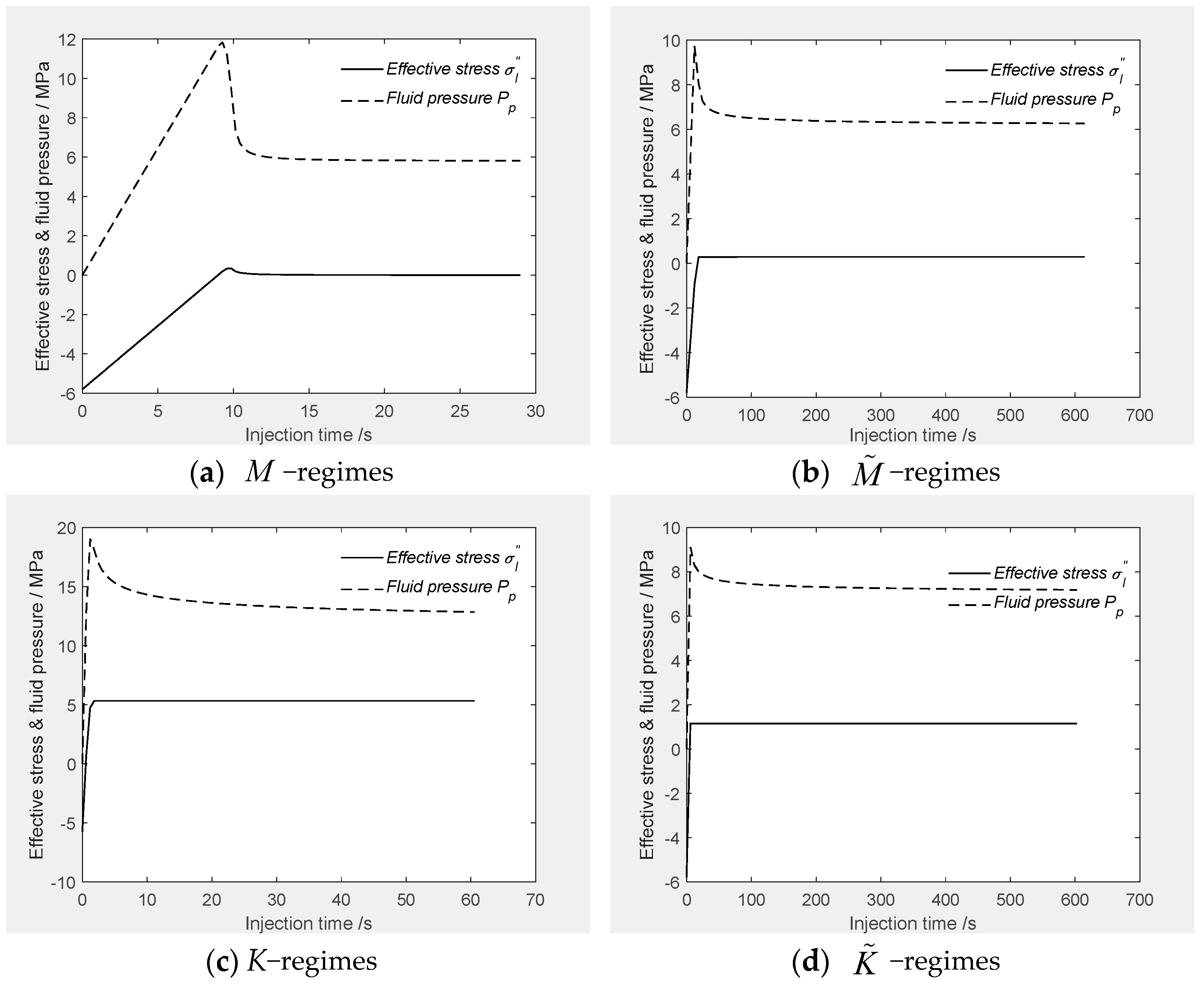
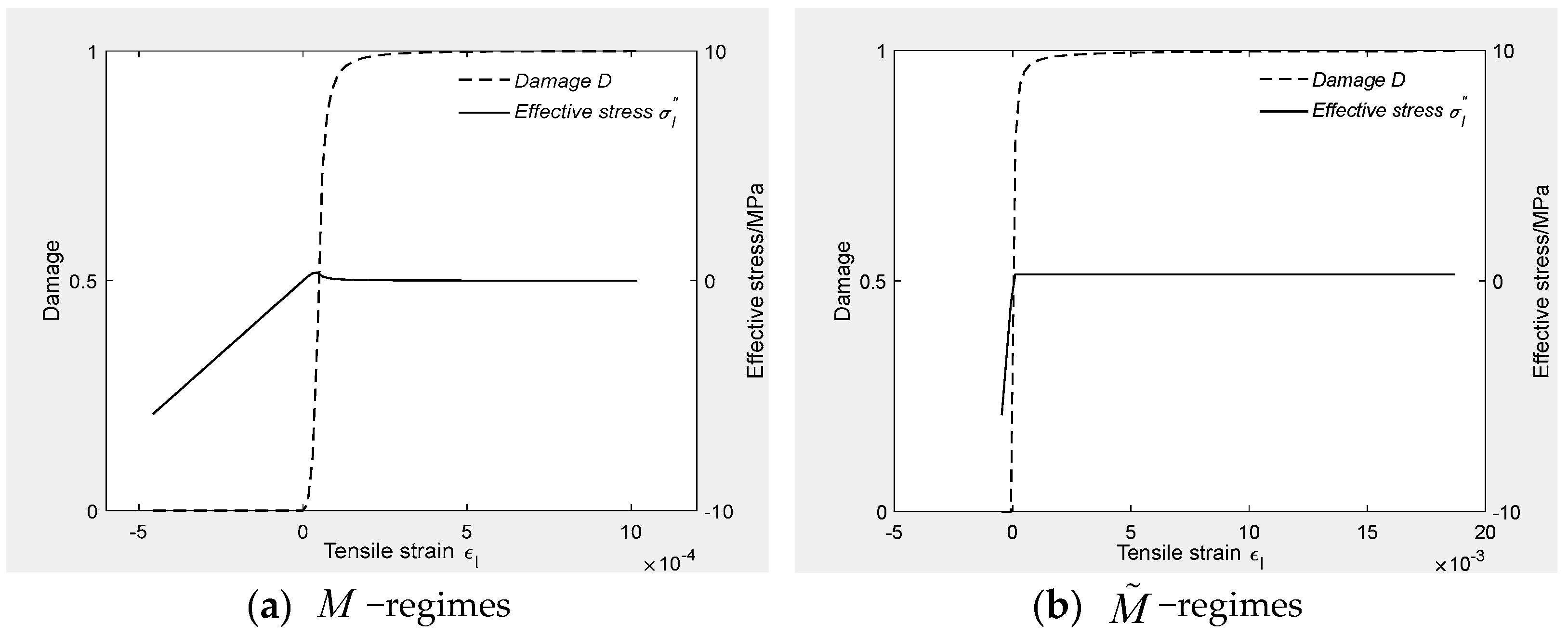
The changes in the skeleton stress (marked as effective stress) and pore pressure are shown in
Figure 6, and the breakdown damage evolution is shown in
Figure 7 (note that the negative strain represents the skeleton initially being under compression). From the comparisons between these plots, it is known that the change law of
inherits the evolution modes of the pore fluid pressure and effective stress, while the change in
inherits the evolution mode of the breakdown damage.
4.3.2. Confining Stress Response
The change in the confining stress
(
) with the fluid injection time in different fracturing regimes is shown in
Figure 8. Generally, the confining stress
first exhibits an inverse law to the skeleton stress and fluid pressure since it was increased from the initial state
; it then rises to a compressive peak and then descends to a low level during compression as the fluid pressure and effective stress are removed.
From the description of the tip process shown in
Figure 1, it is known that the time when the peak confining stress occurs corresponds to the region of the fracture tip where a breakdown is about to occur, and the long time span after the peak corresponds to the whole fracture body. Therefore, from
Figure 8, the confinement of the stress distribution around a fracture can be speculated to be fracturing propagation, while the fracture tip is surrounded by a concentrated zone of the confining compressive stress, with the maximum
in the center. Moreover, the fracture faces are surrounded by a less concentrated compressive zone on each side, with
. (Note that the sign conventions are the following: compressions (
,
, and
) are negative and tensions (
,
,
, and
) are positive.)
The ratios of confining stress to the far-field confining stress, fluid pressure, and skeleton stress in the four limiting regimes are shown in
Table 7, in which
and
are the ratios of the maximum confining stress and steady confining stress after the peak to the far-field confining stress, respectively. From the two extracted ratios, the concentration of the confining stress at the fracture tip and the fracture body can be determined. From the recorded outcomes, the following can be argued: (1) the stress concentrations at the fracture tip are generally larger than in the fractured body for various fracturing regimes; (2) the concentrations in the storage-dominated regimes
and
are larger than in leak-off-dominated regimes
and
for both the fracture tip and body, which shows that the leak-off leads to a decrease in concentration.
4.3.3. Back Stress Effects
In
Table 7,
and
are the ratios of the confining stress to the pore pressure at the fracture tip and body, respectively, and represent the poroelastic effect where pore pressure generates confining stress. They show that at the fracture tip,
approximates to the value of −1, and in the fractured body,
are 1.89 and 1.69 in the viscosity-dominated regimes and 0.73 and 1.03 in the toughness-dominated regimes. This effect indicates that at the fracture tip, confining stress is caused by the pore pressure and is slightly affected by the fracturing regimes. However, in the fractured body, confining stress is strongly affected by the fracturing regimes. In the viscosity-dominated regimes, the breakdown is completed; thus, confining that stress is mainly determined by the channel flow. Nevertheless, in the toughness-dominated regimes, the breakdown is incomplete; confining that stress response is hampered by incomplete cohesive tractions. The completeness of the breakdown is shown in
Table 7, by
and
, where it is demonstrated that the skeleton stress
in the toughness-dominated regime is much larger than that in the viscosity-dominated regimes.
Furthermore, the back stress coefficient
can be calculated as follows [
12]:
, which is listed in
Table 8. Clearly, it shows that back stress exhibits similar characteristics to confining stress.
4.4. The Mechanisms of Confining Stress Response in the Four Limiting Regimes
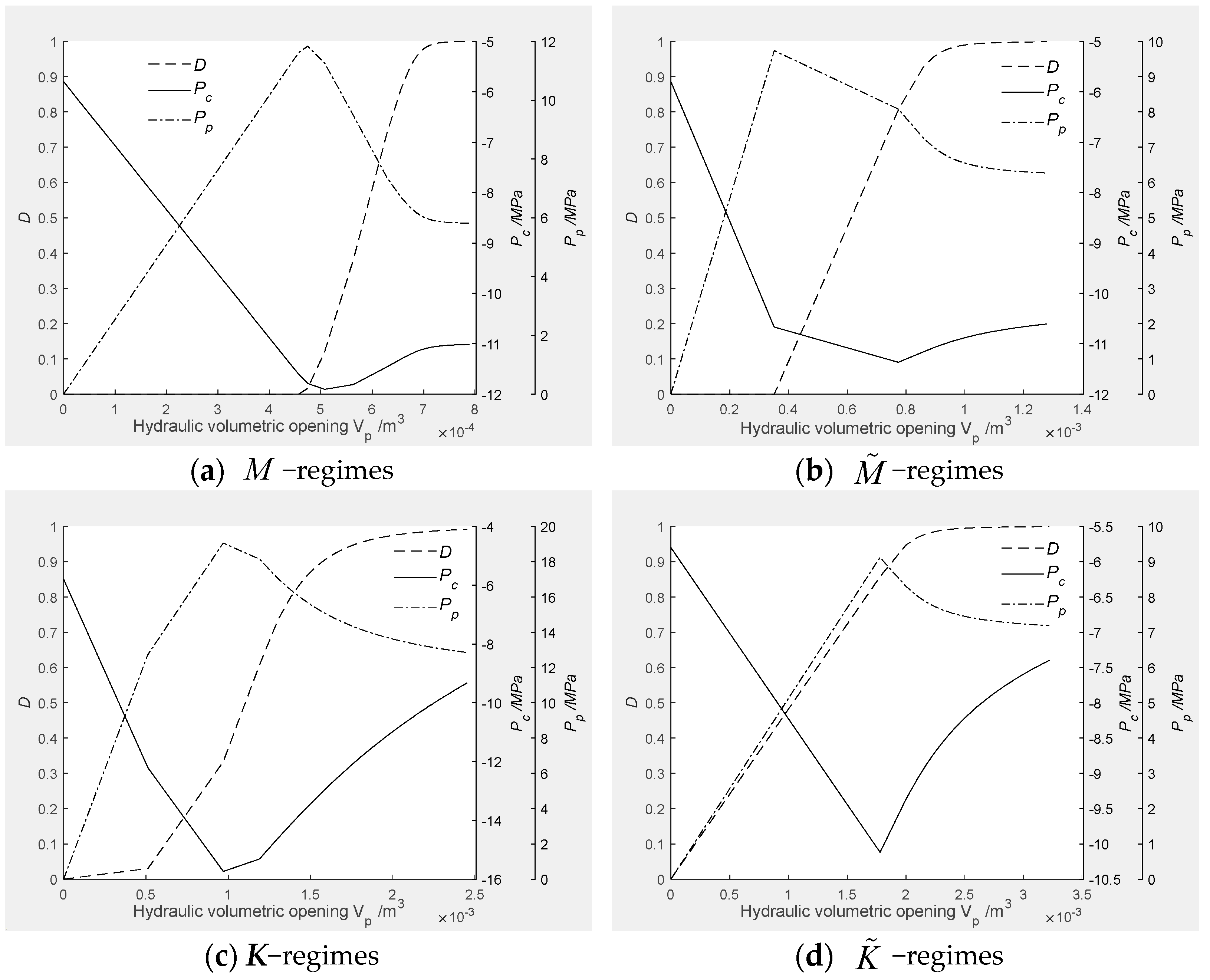
The mechanisms of the confining stress response to the hydraulic volumetric opening can be observed in the plots of
vs.
in
Figure 9 and the comparison of
vs.
,
, and
in various fracturing regimes in
Figure 10.
Morphologically, these plots show similar characteristics to the constitutive relations of the stress vs. strain at anhydrous conditions, where the confining stress response and pore pressure initially increase to a peak, followed by a decrease to a low level as breakdown damage occurs. However, these constitutive responses are strongly governed by the hydraulic fracturing regimes.
One of these features is the peak shifting between the responses of confining stress and the pore pressure. In the viscosity-dominated regimes, the confining stress response lags behind the pore pressure, but in the toughness-dominated regimes, the peak shifting disappears. In addition, leak-off leads to more significant peak shifting in the regime than in the regime.
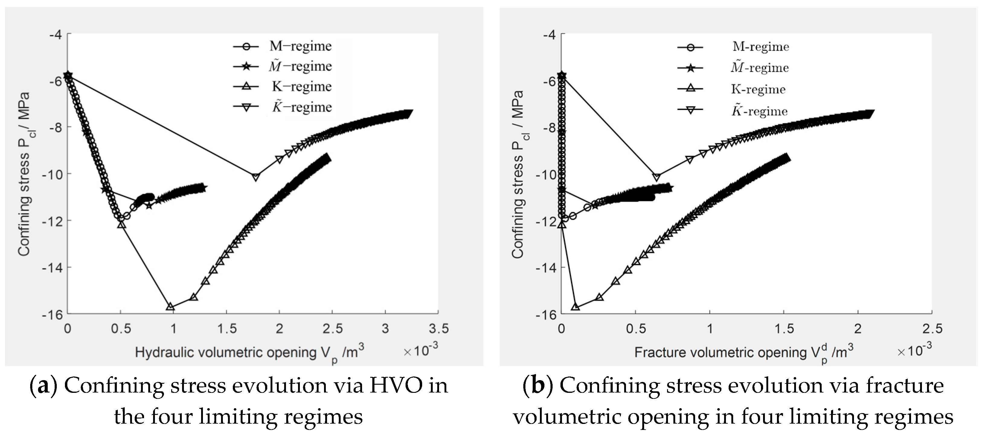
Another feature is that the time spans (measured according to the volumetric opening) of the confining stress responses vary with the various fracturing regimes. As can be ascertained from
Figure 10a, in the viscosity-dominated regimes, the time spans are smaller than those in the toughness-dominated regimes.
The third is that the confining stress response time spans are governed by the synchronization of the evolutions of the pore volumetric opening and fracture volumetric opening.
As can be observed, fluid injection first leads to an increase in the pore pressure and, consequently, to the enhancement of the pore volumetric opening. In turn, confining stress response around the fracture is further stimulated, but as soon as breakdown happens, fracture opening leads to a pore pressure reduction, and, therefore, both the pore volumetric opening and confining stress are decreased.
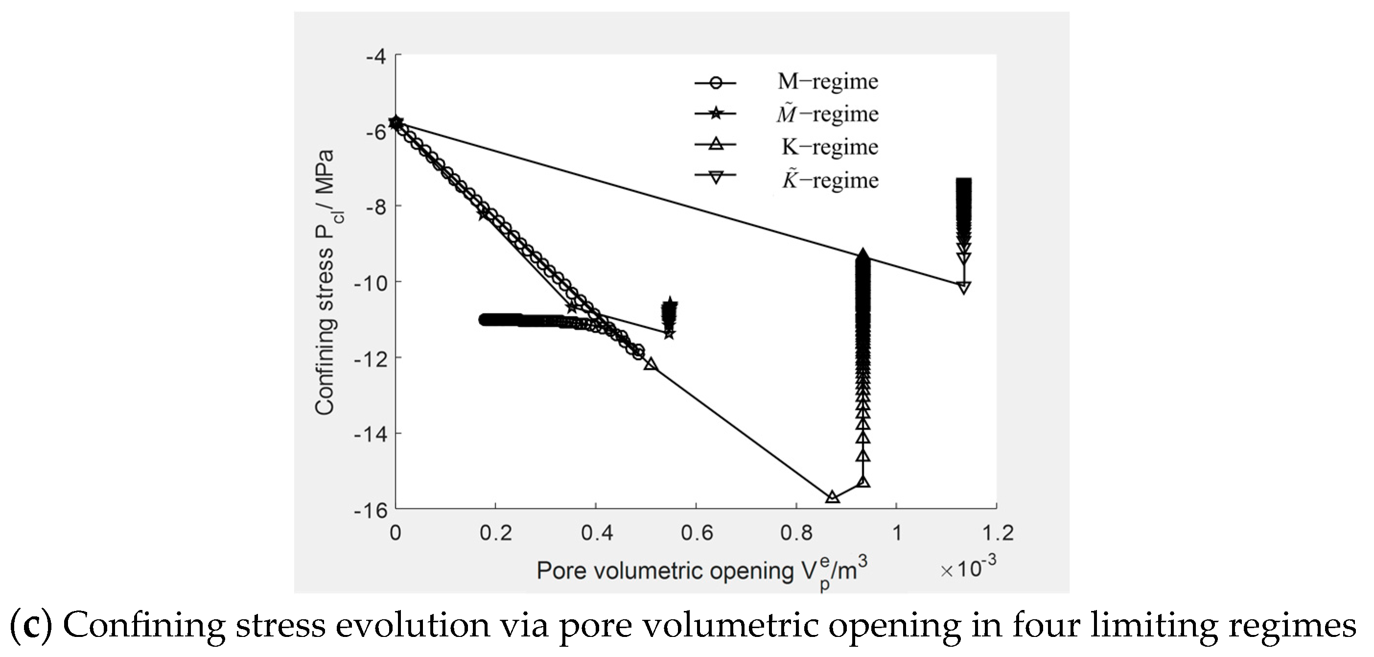
In the
regime, the fracture is brittle, and a clear division line between the evolutions of the pore volumetric opening and fracture volumetric opening can be found, which means that as soon as breakdown begins, the pore volumetric opening stops at once. Therefore, a short peak confining stress response will happen, as is shown in
Figure 11a. Nevertheless, in the
regimes, the evolving of the pore volumetric opening is blended with fracture opening at different degrees, which will lead to the manifestation of ductile fracture and long-peak confining stress responses, as is shown in
Figure 11b–d.
5. Conclusions
In this work, a theoretical framework of hydraulic volumetric opening (HVO) models was clarified, while the expression of the confining stress response was derived. Furthermore, the calculation of the hydraulic volumetric openings and confining stress response was clarified. By employing several examples, the change laws of the hydraulic volumetric openings and confining stress response, poroelastic effects, and constitutive relationships between the confining stress response and hydraulic volumetric openings were demonstrated.
(1) Confining stress concentrations at the fracture tip are generally larger than in the fractured body for varying fracturing regimes.
(2) The concentrations in the storage-dominated regimes and are larger than in the leak-off-dominated regimes and for both the fracture tip and body, which shows that the leak-off leads to a reduction in the concentration.
(3) Poroelastic effects and are slightly affected by fracturing regimes at the fracture tip but strongly affected by fracturing regimes in the fracture body. Their effect will induce a prominent peak shifting between confining stress response and pore pressure in the viscosity-dominated regimes.
(4) The constitutive relationships between the confining stress response and hydraulic volumetric opening are strongly governed by hydraulic fracturing regimes. The time span of the peak confining stress response is shorter in the regime than in the other three limiting regimes.


 and
and 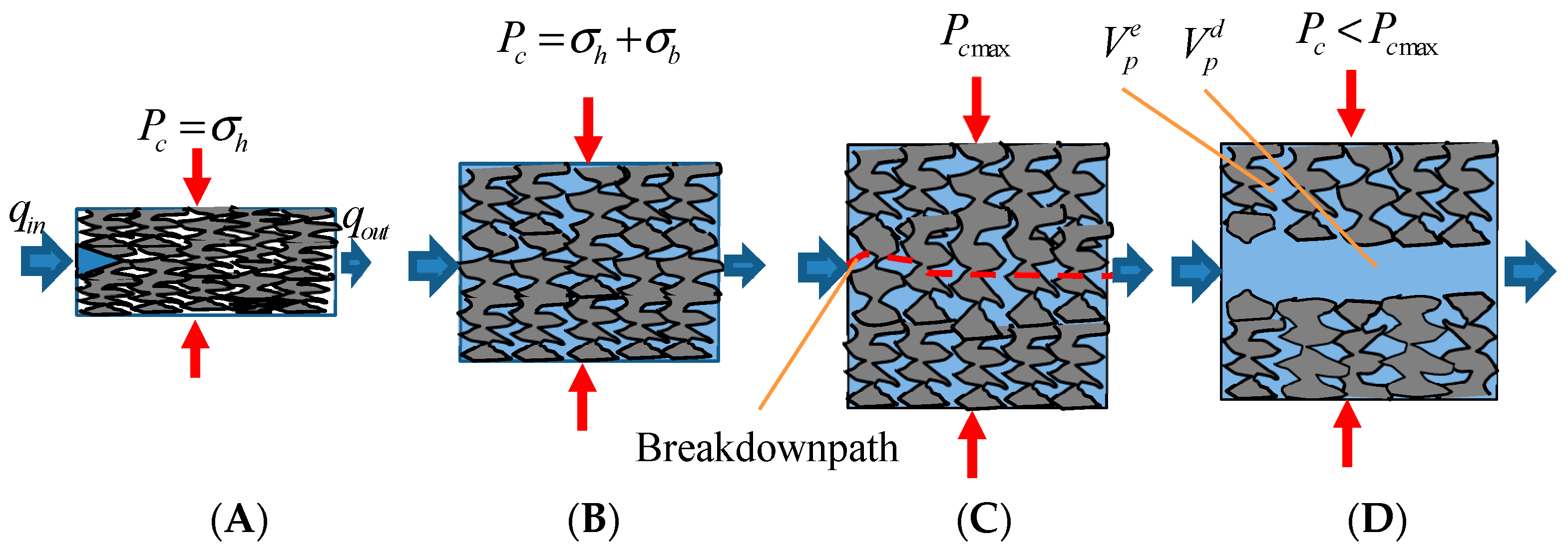


