Article

Study on Parameter Inversion Model Construction and Evaluation Method of UAV Hyperspectral Urban Inland Water Pollution Dynamic Monitoring

1
Changchun Institute of Optics, Fine Mechanics and Physics, Chinese Academy of Sciences, Changchun 130033, China
2
University of Chinese Academy of Sciences, Beijing 100049, China
*
Author to whom correspondence should be addressed.
Water 2023, 15(23), 4131; https://doi.org/10.3390/w15234131
Submission received: 6 October 2023 / Revised: 26 October 2023 / Accepted: 17 November 2023 / Published: 29 November 2023

Abstract

:
The problem of environmental water pollution is becoming increasingly important. Inland rivers and lakes form interconnected water networks with fragile water ecosystems, and urban water pollution problems occur frequently. Chemical oxygen demand (COD), dissolved oxygen (DO), total phosphorus (TP), total nitrogen (TN), and ammonia nitrogen (NH3-N) in inland rivers are important indicators to evaluate water health quality. Timely and accurate reflection of dynamic changes to the key indices of urban river health status are of vital practical significance to adjust water treatment policy and ensure the stability of the aquatic environment and people’s health. This study used COD, DO, TP, TN and NH3-N as typical water quality parameters for a reservoir in Guangxi Province, China and established a set of standardized processes covering UAV hyperspectral sampling and ground spectral correction, spectral data preprocessing, and modeling. In combination with machine learning and statistical analysis, an inversion method for measuring urban inland water pollution from UAV hyperspectral imaging with different dynamic monitoring parameters was proposed. And we compared the different combinations of preprocessing algorithm-regression algorithm and dimensionality reduction algorithm to get a unified model for quantitative estimation of water quality parameter concentration. We evaluated the performance of the proposed model according to root mean square error (RMSE), mean absolute error (MAE), mean absolute percentage error (MAPE), and coefficient of determination ( R 2 ). The experimental results showed that our model was superior to other algorithms in RMSE, MAE, MAPE, and R 2 . The MAPE of this model ranged from 0.01 to 0.12 and R 2 ranged from 0.84 to 0.98 in all water quality parameters. In general, this study provides an effective tool for decision-makers to investigate the source and physical mechanism of water pollution and establish a graded water quality evaluation model.

1. Introduction

Owing to the influence of natural factors and human activities, the water quality of many inland rivers has been severely degraded, which leads to the need for water quality monitoring technology. Traditional water quality monitoring uses manual sampling and testing methods, which are low in monitoring efficiency and consume substantial human and material resources. In addition, isolated monitoring points cannot accurately describe the water quality of the whole water area, nor can they obtain the spatial distribution of water quality. These limitations make it difficult to meet the monitoring needs [1] of modern urban governance systems. Remote sensing of water quality, as an auxiliary to the existing monitoring system, can obtain multi-scale and multi-temporal information on rivers and lakes and help track the location of possible pollution sources. Effective monitoring of water quality changes is important for the protection of urban rivers. In recent years, water quality monitoring models using remote sensing technology have been widely used in the quantitative estimation [2,3] of a variety of water quality parameters, including chemical oxygen demand (COD), dissolved oxygen (DO), total phosphorus (TP), total nitrogen (TN) and ammonia nitrogen (NH3-N). All abbreviations in the text are shown in Abbreviations Index. The accumulation of these elements leads to water eutrophication, changes in turbidity, and increases in total suspended matter content. They directly lead to the rapid accumulation of chlorophyll, which substantially [4] disturbs urban river ecosystems. Therefore, real-time and accurate monitoring of water quality changes, as well as determining pollution sources and mechanisms that cause water quality changes, are crucial to solving the problem of urban inland water pollution and are the basis and priority for protecting the water environment. In recent years, with the rapid development of remote sensing technology, inversion of water quality parameter changes using remote sensing has become a common means of water quality monitoring. Satellite remote sensing technology can effectively monitor large urban rivers, but most urban rivers are less than 100 m in width and belong to the category of small and medium-sized rivers. Village and town rivers are usually less than 10 m in width. There is a dense, widely distributed network of these small and medium-sized rivers, which often have very silted channels with slow flow rates, and illegal and unplanned discharge from the surrounding environment. Therefore, the water quality is prone to deterioration, and there is a high incidence of river pollution. These conditions increase the need for high spatial and temporal resolution remote sensing data. The existing satellite-borne remote sensing monitoring methods often cannot meet the monitoring needs of modern urban river and lake water environments. In terms of analysis, a variety of methods have been used to monitor water quality, including deep learning methods such as empirical methods, convolutional neural networks (CNN), deep convolutional generation and adversarial networks, and Bayesian neural networks. Most of these grade [5,6,7,8] water quality according to the concentration of water quality parameters and achieve relatively good performance. However, the spatial resolution of the above studies is relatively poor, and the water quality cannot be monitored in a small range. Therefore, it cannot be applied to the monitoring of water pollution in small inland water bodies in cities. Some researchers, such as Bonansea et al., have studied satellite data to monitor the change in water quality parameters through polynomial regression modeling, using the relationship between spectra. Similarly, Gu et al. used two GF-5 hyperspectral images to estimate chlorophyll a concentration and suspended sediment concentration in the Yangtze River Estuary and [9,10,11] obtained a prediction accuracy of 0.815. However, this kind of method requires many data sets as training data to obtain relatively good prediction results, which results in a long data collection period and limited accuracy. By improving the traditional CNN research for the prediction of COD concentration using hyperspectral remote sensing and a gated recurrent neural network (GRNN), WANG et al. achieved good modeling performance [12,13]. However, their data were simulated in the laboratory which may not have practical significance. In recent years, researchers have studied the use of low-altitude remote sensing technology from unmanned aerial vehicles (UAV), and have used UAV to monitor chlorophyll a. Jung Min Ahn achieved good results in predicting cyanobacteria blooms in controlled rivers using hyperspectral images combined with machine learning [14,15,16,17,18,19]. In summary, there are few studies on inversion methods for UAV hyperspectral dynamic monitoring parameters for urban inland water pollution in China and elsewhere. And the analysis algorithm is inefficient. In view of this, remote sensing inversion models of spectral features of water quality parameters were constructed by taking COD, DO, TP, TN and NH3-N for five typical water quality parameters in Beihai City, Guangxi Province as research objects through different pretreatment and regression methods. In this study, the water pollution index in a reservoir was quantitatively and dynamically monitored by mining the spectral information in the wavelength range of 400–1000 nm obtained by the UAV hyperspectral imaging system. And we compared different combinations of pre-processing algorithm, regression algorithm and dimensionality reduction algorithm, and finally establishes a unified model of quantification of the concentration of the water quality parameters to be used for the effective quantitative estimation of the concentration of water quality parameters, so as to achieve the quantitative and dynamic monitoring of water pollution indexes in the water reservoirs.The specific studies were to: (1) obtain the spectral data of the hyperspectral image in the range of 400–1000 nm; (2) eliminate the interference from the instrument itself and the surrounding environment by selecting suitable spectral preprocessing; (3) find different combinations of preprocessing and regression algorithms for different monitoring indicators, and study ways of evaluating the performance of the models in the process; (4) through three methods—principal component analysis (PCA), continuous projection algorithm (SPA) and simulated annealing algorithm (SAA)—to select the best wavelength combination to optimize the inversion model and improve inversion efficiency. This approach can achieve the rapid monitoring of water pollution indicators for COD, DO, TP, TN and NH3-N, to establish a comprehensive analysis model.

2. Materials and Methods

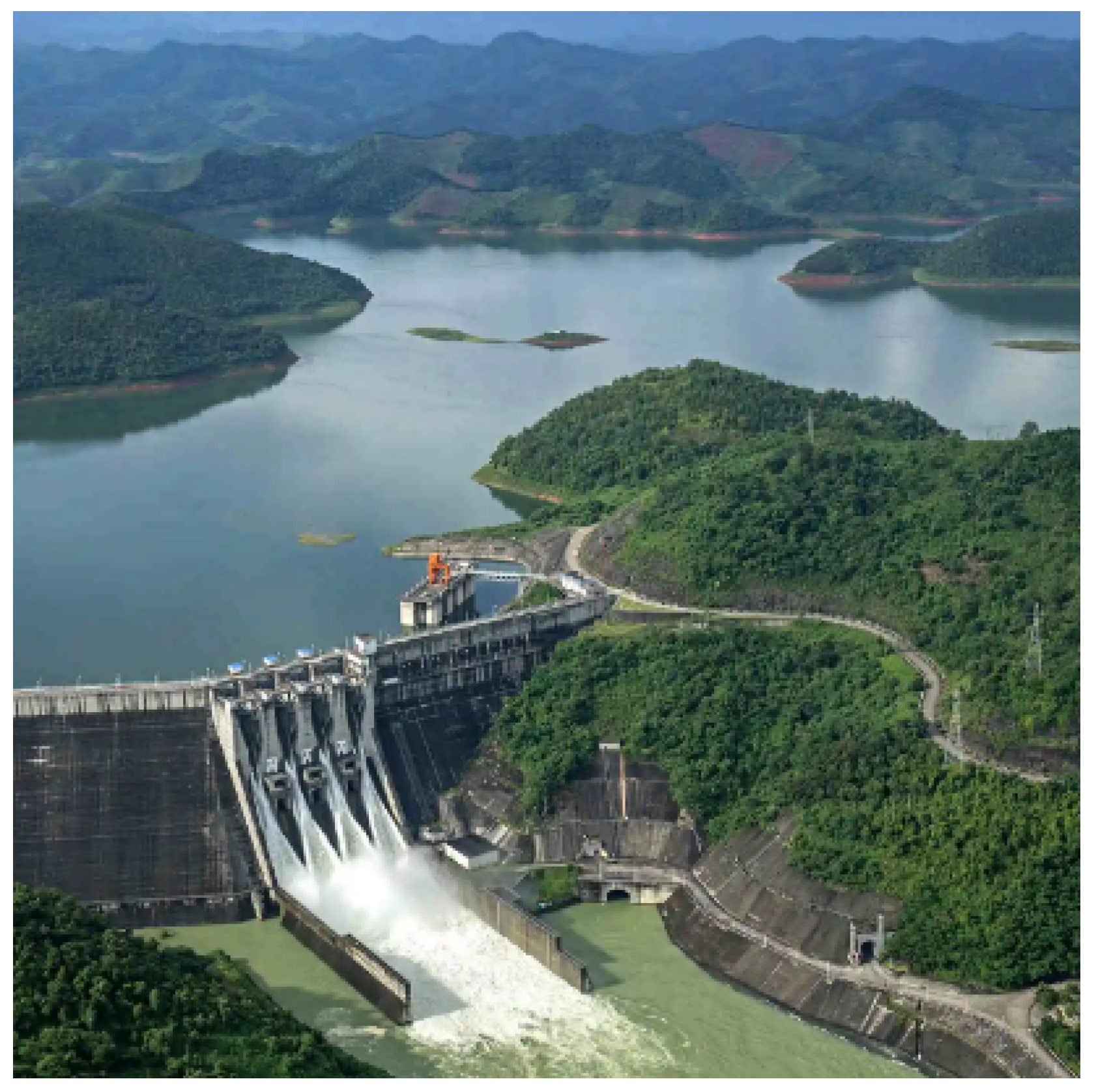
2.1. Study Area Overview

In this study, a reservoir in Guangxi Province was selected as the research area. The reservoir is a centralized drinking water source at the Beihai level, located on the Sanhe River, with a normal reservoir capacity of 11.53 million m3 (Figure 1). Analysis of the reservoir is helpful to understand the ecological environment status of the Beijiao water plant and provide for the safety of the urban water supply. Hyperspectral images were taken at multiple points in five different water sections in the reservoir, including the village on the lower slope, the Poxinling, the Caohualing, the head of the dam, and the reservoir (Table 1). At the same time, ground spectral data were collected by a micro-optical fiber spectrometer in the same water area. Water samples were collected using a cup-type fixed- depth water quality sampler in the experimental area. There were 20 sampling points in a single experiment, and 500 mL water samples were collected at each point. The samples were sent to professional institutions for testing according to the national standard, and the measured data of the detected content of COD, DO, TP, TN and NH3-N were used as the standard for subsequent spectral modeling.

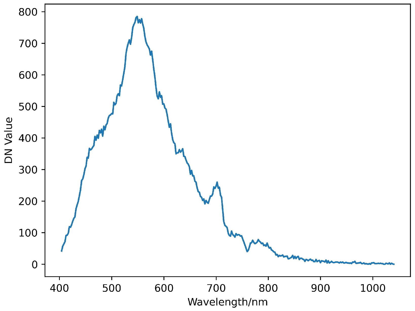
2.2. UAV Hyperspectral Data Acquisition and Preprocessing

In this study, we used an unmanned airborne hyperspectral imaging system integrated by Hangzhou Hyperspectral Imaging Technology Co., Ltd. (Hangzhou, China) as shown in Figure 2b. The core spectral module of the system was independently developed by CIOMP.
The spectral range covered 400–1000 nm, the spectral resolution was better than 3 nm, and the focal length of the lens (kowa) was 35 mm. The spectral range of the miniature optical fiber spectrometer covered 200–1100 nm, and the spectral resolution was better than 1.5 nm. The hyperspectral image of the waters of Niuweiling, Guangxi was collected in reflection mode, and the spectral curve of the water body was obtained, as shown in Figure 3. The processing process is shown in Figure 4.

2.3. ROI Selection and Pretreatment Method

The experiment time was between 10:00 and 14:00 in the day. During the experiment, a high reflectivity image was obtained by scanning the gradient reflectivity whiteboard, and the hyperspectral image data of five different water areas in the reservoir were collected. The reflectivity of the reservoir water was corrected using Formula (1):
I R = ( I O I B ) / ( I W I B )
where, I R represents the corrected reflectivity hyperspectral image data, I O represents the original water body hyperspectral image data, I W represents the reflectivity whiteboard hyperspectral image data taken under the same experimental environment, I B represents the reflectivity dark plate hyperspectral image data taken in the same experimental environment.
The micro-optical fiber spectrometer self-developed by CIOMP was used to correct the hyperspectral image data according to Formula (2).
R = r 1 , 1 r 1 , 2 r 1 , 3 r 1 , n r 2 , 1 r 2 , 2 r 2 , 3 r 2 , n r 3 , 1 r 3 , 2 r 3 , 3 r 3 , n r m , 1 r m , 2 r m , 3 r m , 4 r 1 , 1 r 1 , 2 r 1 , 3 r 1 , n r 2 , 1 r 2 , 2 r 2 , 3 r 2 , n r 3 , 1 r 3 , 2 r 3 , 3 r 3 , n r m , 1 r m , 2 r m , 3 r m , 4 = R
A modified model of UAV reflectance and ground reflectance was established, where n is the number of bands, m is the number of sample points, and r is the original hyperspectral reflectance. The processed hyperspectral image is shown in Figure 5.
In this study, 50 points in each of the above five regions were selected for water sampling. Of the data points, 70% were randomly selected as the training set and the remaining 30% were the prediction set. Before analyzing the ROI, it was necessary to preprocess the data to eliminate the system noise and the influence of the surrounding environment. In this study, SNV, MSC, WAVE, MMS and cascade were used for pre-processing. SNV and MSC can reduce the influence of the scattering on the spectrum owing to the uneven particle distribution and different particle size. The effects of some of the different pretreatment methods are shown in Figure 6.

3. Analytical Model and Evaluation Criteria

3.1. Modeling Methods for the Full Spectrum Regression Model

In this study, LR, SVR, PLSR and RFR regression algorithms were used to model and analyze the COD, DO TN, TP, and NH3-N content and spectral reflectance data in a reservoir water body. LR is used where the relationship between variables is simple. SVR is carried out by finding an optimal curve or hyperplane in the data set, that is, by minimizing the training error and maximizing the effective edge [20,21]. SVR regression uses a kernel function to deal with nonlinear problems, which makes it easier to separate input samples. It has strong nonlinear fitting ability and robustness, and only calculates the support vector in the prediction. This greatly reduces the computation process. For the training data set, D = ( x , y ) , where x i is the n-dimensional and y i the scalar predicted value, the relaxation variable sum is introduced to minimize the objective function as follows: ξ i ξ i *
F = min 1 2 ω 2 + C i = 1 n ( ξ i + ξ i * )
where: C is the penalty coefficient; w and b are the coefficient and intercept of the model respectively. Kernel functions commonly introduced include Gaussian kernel, polynomial kernel and sigmoid kernel function. Here, the Gaussian kernel function was selected for modeling in the study, as shown in Equation (4):
K ( x i , x j ) = exp ( x i x j 2 ) / ( 2 σ 2 )
where: σ is a hyperparameter. PLSR is a regression modeling method for multi-dependent variables to multi-independent variables. The final model contained all the original independent variables, and had good model interpretability [22,23]. RFR is composed of multiple regression trees, and there is no correlation between each decision tree in the forest. The final output of the model is determined by all decision trees in the forest, which has strong anti-interference ability and anti-overfitting ability [24,25,26,27,28,29,30].
In this study, the root-mean-square error(RMSE), mean absolute error (MAE) and determination coefficient ( R 2 ) were used to evaluate the effect of the regression analysis model. In general, the smaller the RMSE and MAE error and the closer the R 2 is to 1, the better the prediction performance of the model. The specific parameters are calculated as follows:
R M S E = 1 m i = 1 m ( y i y ^ l ) 2 1 / 2
M A E = 1 m i = 1 m | y i y ^ i |
R 2 = i = 1 m ( y ^ l y ¯ l ) 2 i = 1 m ( y i y ¯ l ) 2
where, RMSE represents the root mean square error, MAE represents the average absolute value error, R 2 represents the determination coefficient, m represents the number of data points, y i represents the true value of the key indicator content in the water body data point, y ^ i represents the predicted value of the key data indicators COD, DO, TN, TP, and NH3-N, content, y ¯ i represents the average value of the true content of key indicators COD, DO, TN, TP, and NH3-N in each data point set.
The expected values of the COD, DO, TN, TP, and NH3-N contents of different key indicators obtained by full-spectrum modeling are shown in Table 2, Table 3, Table 4, Table 5 and Table 6, and the average absolute error percentage of predicted values of water quality parameters is shown in Figure 7.
A smaller MAPE indicates a better prediction by the model. On the basis of the above tables and graphs and combining the RMSE and MAE data, we found that the best prediction model of COD was established by the combination of MSC preprocessing and the RandomForest regression algorithm, while the best prediction model of DO was established by the combination of WAVE preprocessing and the SVR regression algorithm. The best prediction model of NH3-N was established by the combination of MSC+SNV pretreatment and PLS regression algorithm, while the best prediction model of TP was established by the combination of MSC+SNV pretreatment and the RandomForest regression algorithm. The best prediction model of TN was established by the combination of MMS pre-processing and the PLS regression algorithm. All these factors provided data input for the following research.

3.2. Spectrum Dimensionality Reduction

The spectral dimension reduction methods used in this study included SPA, PCA, and SAA. SPA is one of the commonly used wavelength selection methods, which can select the shortest collinear wavelength combination. For COD parameter prediction, in this study, the MSC-RFR analysis model was established with each wavelength group, and the wavelength combination with the largest determination coefficient was taken to be the best combination. In this study, a total of 20 characteristic wavelengths were selected by SPA. The wavelength combination was selected by PCA by extracting the principal component which contributed the most to the original information and combining the corresponding principal component load coefficient. In this study, the PCA algorithm was used to select 15 characteristic wavelengths. SAA is a random combinatorial optimization algorithm, which considers not only the optimal solution, but also the deteriorating solution within a certain limit, finds the local optimal solution, and then obtains the global optimal solution. In this study, SAA was used to select 20 characteristic wavelengths, and the optimal wavelength combination selected by SPA, PCA, and SAA was used to simplify the MSC-RFR model. The MSC-SPA-RFR model, MSC-PCA-RFR model, and MSC-SAA-RFR model were established. The other four water quality parameters were calculated in the same way, and their specific performance is shown in Table 7.

4. Results and Discussion

Part 3 shows that we were able to establish corresponding preprocessing and full-spectrum regression modeling methods for the indicators COD, TN, TP, NH3-N, and DO, as can be seen from Table 2, Table 3, Table 4, Table 5 and Table 6 above. As can be seen from Table 7, for COD, the MSC method was used to pretreat the hyperspectral reflectance data of reservoir water, and the MSC-RFR analysis model was established. RMSE, MAE, R 2 and MAPE were used to evaluate the full spectrum analysis model. Then, three different dimensionality reduction methods were used to reduce the spectral dimension of the reservoir water hyperspectral reflectance data to establish the MSC-SAA-RFR, MSC-SPA-RFR, and MSC-SPA-RFR analysis models. Comparison of the experimental results showed that the MSC-SAA-RFR model had a higher R 2 value and a lower MAPE value and could better predict the COD content in water. For DO, the WAVE-SVR full spectrum analysis model was first established, and then three different dimensionality reduction methods were used to reduce the spectral dimension of reservoir water hyperspectral reflectance data to establish the WAVE-SAA-SVR, WAVE-SPA-SVR, and WAVE-PCA-SVR analysis models. The comparative experimental results showed that the WAVE-SAA-SVR model had a higher R 2 value and lower MAPE value, which could better predict the DO content in water. For NH3-N, the full spectrum analysis model of MSC-PLS was first established, and then three different dimensionality reduction methods were used to reduce the spectral dimension of the reservoir water hyperspectral reflectance data to establish the MSC+SNV-SAA-PLS, MSC+SNV-SPA-PLS, MSC+ SNV-PACC-PLS analysis models. The comparison of the three experimental results showed that the MSC+SNV-SAA- PLS model had a higher R 2 value and lower MAPE value, and could better predict the NH3-N content in water. For TP, the full spectrum analysis model of MSC-RFR was first established, and then spectral dimension reduction was performed on the hyperspectral reflectance data of reservoir water by three different dimensionality reduction methods to establish the MSC+SNV-SAA-RFR, MSC+SNV-SPA-RFR, and MSC+SNV-PCA-RFR analysis models. Comparing the three experimental results showed that the MSC+SNV-SPA-RFR model had a higher R 2 value and lower MAPE value, which could better predict the TP content in water. For TN, the full spectrum analysis model of MMS-PLS was first established, and then three different dimensionality reduction methods were used to reduce the spectral dimension of the reservoir water hyperspectral reflectance data to establish the MMS-SAA-PLS, MMS-SPA-PLS, and MMS-PCA-PLS analysis models. The comparative experimental results of the three showed that the MMS-PCA-PLS model had a higher R 2 value and lower MAPE value, which could better predict the TP content in the water body. In addition, we believe that the quality of the evaluation model was not determined by a single level of R 2 and RMSE. Only through the comprehensive evaluation of R 2 , RMSE, and MAPE could a more robust water quality parameter analysis model be obtained.

5. Conclusions

Because the detection indicators of urban river sewage cannot be monitored over a large area quickly and dynamically, this study used a UAV to collect hyperspectral image data, which was effective and flexible, with a higher spatial resolution and less medium interference than satellite collection. Combining machine learning and statistical analysis, we examined the parameter inversion method for dynamic monitoring of urban inland water pollution on the basis of UAV hyperspectral imaging technology. At the same time, we established a set of standardized processes from UAV hyperspectral sampling, ground spectrum correction, spectral data preprocessing, and modeling. We combined the above-mentioned models into a unified end-to-end structure. In general, from the perspective of theoretical significance, this study perfected a set of systematic data collection, physical and chemical analysis of water samples, spectral preprocessing, and data modeling of the key indicators of water quality parameters, providing a guideline for subsequent research. From the perspective of application significance, this method can monitor the change in urban river water quality in real time which is conducive to the tracking of pollution sources, and provide a decision-making basis for urban river water environment management by establishing an early warning system. This will minimize the harm caused by sewage to people’s lives.
However, this research has some limitations. On the one hand, the data for our study were collected between 10:00 a.m. and 2:00 p.m. on sunny days, which did not include monitoring during some extreme bad weather. In the follow-up work, we plan to add weather and other parameter factors into the model to correct this, further improve the robustness of the analysis and prepare for all-weather monitoring. On the other hand, we will conduct experiments in China and other parts of the world to further verify the effectiveness of the quantitative method of water quality parameter concentration in this study, and accelerate the construction of and intelligent monitoring system of water environment.

Author Contributions

Conceptualization, J.C. and J.W.; Methodology, C.S.; Software, M.W.; Validation, J.C., J.W. and Z.Z.; Formal analysis, Z.Z.; Investigation, J.W.; Resources, J.Y.; Data curation, C.S.; Writing—original draft preparation, J.C.; Writing—review and editing, J.C.; Visualization, S.F.; Supervision, J.Y.; Project administration, N.S.; Funding acquisition, J.C. All authors have read and agreed to the published version of the manuscript.

Funding

Jilin Province and the Chinese Academy of Sciences Science and Technology Cooperation in High-tech Industrialisation Special Funds Project (2022SYHZ0025); Jilin Province Science & Technology Development Program Project in China (20200403009SF).

Data Availability Statement

Data underlying the results presented in this paper are not publicly available at this time but may be obtained from the authors upon reasonable request.

Conflicts of Interest

The authors declare no conflict of interest.

Abbreviations

The following abbreviations are used in this manuscript:
CODChemical Oxygen Demand
DODissolved Oxygen
TPTotal Phosphorus
TNTotal Nitrogen
NH3-NAmmonia Nitrogen
UAVUnmanned Aerial Vehicle
RMSERoot Mean Square Error
MAPEMean Absolute Percentage Error
MAEMean Absolute Error
R 2 Coefficient of Determination
CNNConvolutional Neural Network
DCGANDeep Convolutional Generation and Adversarial Network
BNNBayesian Neural Network
SSCSuspended Sediment Concentration
GRNNGated Recurrent Neural Network
Chl-aChlorophylL-A
PCAPrincipal Component Analysis
SPASuccessive Projections Algorithm
SAASimulated Annealing Algorithm
CIOMPChangchun Institute of Optics, Fine Mechanics and Physics, Chinese Academy of Sciences
ROIRegion of Interest
SNVStandard Normal Variate Correction
MSCMultiplicative Scatter Correction
MMSMin-Max Standardization
WAVEWavelet Transform
LRLinearRegression
SVRSupport Vector Regression
PLSPartial Least Squares Regression
RFRRandom Forest Regression

References

  1. Palmer, S.C.; Kutser, T.; Hunter, P.D. Remote sensing of inland waters: Challenges, progress and future directions. Remote Sens. Environ. 2015, 157, 1–8. [Google Scholar]
  2. Harish, B.; Manjulavani, K.; Shantosh, M.; Supriya, V.M. Change detection of land use and land cover using remote sensing techniques. In Proceedings of the 2017 IEEE International Conference on Power, Control, Signals and Instrumentation Engineering (ICPCSI), Chennai, India, 21–22 September 2017; pp. 2806–2810. [Google Scholar]
  3. HaRa, J.; Atique, U.; An, K.G. Multiyear links between water chemistry, algal chlorophyll, drought-flood regime, and nutrient enrichment in a morphologically complex reservoir. Int. J. Environ. Res. Public Health 2020, 17, 3139. [Google Scholar]
  4. Lewis, W.M., Jr.; Wurtsbaugh, W.A.; Paerl, H.W. Rationale for control of anthropogenic nitrogen and phosphorus to reduce eutrophication of inland waters. Environ. Sci. Technol. 2011, 45, 10300–10305. [Google Scholar]
  5. Adamiak, M.; Będkowski, K.; Majchrowska, A. Aerial imagery feature engineering using bidirectional generative adversarial networks: A case study of the pilica river region, Poland. Remote Sens. 2021, 13, 306. [Google Scholar]
  6. Doña, C.; Chang, N.B.; Caselles, V.; Sánchez, J.M.; Camacho, A.; Delegido, J.; Vannah, B.W. Integrated satellite data fusion and mining for monitoring lake water quality status of the Albufera de Valencia in Spain. J. Environ. Manag. 2015, 151, 416–426. [Google Scholar]
  7. Ghaderi, D.; Rahbani, M. Tracing suspended matter in Tiab estuary applying ANN and Remote sensing. Reg. Stud. Mar. Sci. 2021, 44, 101788. [Google Scholar] [CrossRef]
  8. Dona, C.; Sanchez, J.M.; Caselles, V.; Domínguez, J.A.; Camacho, A. Empirical relationships for monitoring water quality of lakes and reservoirs through multispectral images. IEEE J. Sel. Top. Appl. Earth Obs. Remote Sens. 2014, 7, 1632–1641. [Google Scholar] [CrossRef]
  9. Bonansea, M.; Ledesma, M.; Rodriguez, C.; Pinotti, L. Using new remote sensing satellites for assessing water quality in a reservoir. Hydrol. Sci. J. 2019, 64, 34–44. [Google Scholar] [CrossRef]
  10. Bao, Y. Diurnal variation of chlorophyll a concentration in Taihu Lake based on GOCI image classification. Spectrosc. Spectr. Anal. 2016, 36, 2562–2567. [Google Scholar]
  11. Gu, Q.; Li, Q.; Zhou, M. Water Quality Monitoring of the Yangtze Estuary by Using GF-5 Hyperspectral Image. In Proceedings of the 2019 12th International Congress on Image and Signal Processing, BioMedical Engineering and Informatics (CISP-BMEI), Suzhou, China, 19–21 October 2019; pp. 1–5. [Google Scholar] [CrossRef]
  12. Jichang, T.; Xueqin, Y.; Chaobo, C.; Song, G.; Jingcheng, W.; Cheng, S. Water quality prediction model based on GRU hybrid network. In Proceedings of the 2019 Chinese Automation Congress (CAC), Hangzhou, China, 22–24 November 2019; pp. 1893–1898. [Google Scholar] [CrossRef]
  13. Du, C.; Wang, Q.; Li, Y.; Lyu, H.; Zhu, L.; Zheng, Z.; Wen, S.; Liu, G.; Guo, Y. Estimation of total phosphorus concentration using a water classification method in inland water. Int. J. Appl. Earth Obs. Geoinf. 2018, 71, 29–42. [Google Scholar] [CrossRef]
  14. Ahn, J.M.; Kim, B.; Jong, J.; Nam, G.; Park, L.J.; Park, S.; Kang, T.; Lee, J.K.; Kim, J. Predicting Cyanobacterial Blooms Using Hyperspectral Images in a Regulated River. Sensors 2021, 21, 530. [Google Scholar]
  15. Flynn, K.F.; Chapra, S.C. Remote Sensing of Submerged Aquatic Vegetation in a Shallow Non-Turbid River Using an Unmanned Aerial Vehicle. Remote Sens. 2014, 6, 12815–12836. [Google Scholar]
  16. Pajares, G. Overview and Current Status of Remote Sensing Applications Based on Unmanned Aerial Vehicles (UAVs). Photogramm. Eng. Remote Sens. 2015, 81, 281–329. [Google Scholar] [CrossRef]
  17. Su, T.C.; Chou, H.T. Application of Multispectral Sensors Carried on Unmanned Aerial Vehicle (UAV) to Trophic State Mapping of Small Reservoirs: A Case Study of Tain-Pu Reservoir in Kinmen, Taiwan. Remote Sens. 2015, 7, 10078–10097. [Google Scholar]
  18. Zaman, B.; Jensen, A.M.; Clemens, S.; McKee, M. Retrieval of Spectral Reflectance of High Resolution Multispectral Imagery Acquired with an Autonomous Unmanned Aerial Vehicle: AggieAir™. Photogramm. Eng. Remote Sens. 2014, 80, 1139–1150. [Google Scholar]
  19. Su, T.C. A study of a matching pixel by pixel (MPP) algorithm to establish an empirical model of water quality mapping, as based on unmanned aerial vehicle (UAV) images. Int. J. Appl. Earth Obs. Geoinf. 2017, 58, 213–224. [Google Scholar] [CrossRef]
  20. Pour, S.H.; Shahid, S.; Chung, E.S.; Wang, X.J. Model output statistics downscaling using support vector machine for the projection of spatial and temporal changes in rainfall of Bangladesh. Atmos. Res. 2018, 213, 149–162. [Google Scholar] [CrossRef]
  21. Zhang, X.; Liu, G.; Wang, H.; Li, X. Application of a Hybrid Interpolation Method Based on Support Vector Machine in the Precipitation Spatial Interpolation of Basins. Water 2017, 9, 760. [Google Scholar] [CrossRef]
  22. Leone, A.P.; Viscarra-Rossel, R.A.; Amenta, P.; Buondonno, A. Prediction of soil properties with PLSR and vis-NIR spectroscopy: Application to mediterranean soils from Southern Italy. Curr. Anal. Chem. 2012, 8, 283–299. [Google Scholar] [CrossRef]
  23. Hou, L.; Li, X.; Li, F. Hyperspectral-based Inversion of Heavy Metal Content in the Soil of Coal Mining Areas. J. Environ. Qual. 2019, 1, 57–63. [Google Scholar] [CrossRef]
  24. Shi, C.; Liao, D.; Zhang, T.; Wang, L. Hyperspectral Image Classification Based on Expansion Convolution Network. IEEE Trans. Geosci. Remote Sens. 2022, 60, 1–16. [Google Scholar] [CrossRef]
  25. Xi, J.; Ersoy, O.K.; Cong, M.; Zhao, C.; Qu, W.; Wu, T. Wide and Deep Fourier Neural Network for Hyperspectral Remote Sensing Image Classification. Remote Sens. 2022, 14, 2931. [Google Scholar] [CrossRef]
  26. Vaiphasa, C.; Skidmore, A.K.; de Boer, W.F.; Vaiphasa, T. A hyperspectral band selector for plant species discrimination. ISPRS J. Photogramm. Remote Sens. 2007, 62, 225–235. [Google Scholar] [CrossRef]
  27. Xu, Y.; Du, Q.; Younan, N. Particle swarm optimization-based band selection for hyperspectral target detection. In Proceedings of the 2016 IEEE International Geoscience and Remote Sensing Symposium (IGARSS), Beijing, China, 10–15 July 2016; pp. 5872–5875. [Google Scholar] [CrossRef]
  28. Zhao, W.; Wang, L.; Zhang, Z. A novel atom search optimization for dispersion coefficient estimation in groundwater. Future Gener. Comput. Syst. 2019, 91, 601–610. [Google Scholar] [CrossRef]
  29. Zhong, K.; Luo, Q.; Zhou, Y.; Jiang, M. TLMPA: Teaching-learning-based Marine Predators algorithm. AIMS Math. 2021, 6, 1395–1442. [Google Scholar] [CrossRef]
  30. Hennessy, A.; Clarke, K.; Lewis, M. Hyperspectral Classification of Plants: A Review of Waveband Selection Generalisability. Remote Sens. 2020, 12, 113. [Google Scholar] [CrossRef]
Figure 1. Map of distribution of sampled waters.
Water 15 04131 g001
Figure 2. Experimental instrument: (a) UAV hyperspectral imaging system, and (b) miniature fiber optic spectrometer.
Water 15 04131 g002
Figure 3. Spectral reflectance curve of the water body.
Water 15 04131 g003
Figure 4. Water sample data processing flow.
Water 15 04131 g004
Figure 5. Hyperspectral image of the studied water area.
Water 15 04131 g005
Figure 6. Spectral curve of water data: (a) Spectral curve of original data, (b) spectral curve of SNV pretreatment. (c) Spectral curve after MSC pretreatment, (d) spectral curve after SNV+MSC pretreatment, (e) spectral curve after MSC+SNV pretreatment, (f) spectral curve after WAVE pretreatment, (g) spectral curve after MMS pretreatment.
Water 15 04131 g006aWater 15 04131 g006b
Figure 7. Histogram of prediction and evaluation of water quality parameters: (a) MAPE cluster histogram of predicted COD, (b) MAPE cluster histogram of predicted DO, (c) MAPE cluster histogram of predicted NH3-N, (d) MAPE cluster histogram of predicted TP, (e) MAPE cluster histogram of predicted TN.
Water 15 04131 g007aWater 15 04131 g007bWater 15 04131 g007c
Table 1. Water quality monitoring at the center point of the reservoir basin.
Serial NumberSection NameLatitude (N)Longitude (E)
1In the library21.596800900 109.232536650
2Downhill Village21.607201300 109.237450290
3Caohualing Village21.60265254 109.240883460
4Slope Heart Ridge21.612006920 109.230904750
5Dam Head21.589200229 109.229440652
Table 2. Prediction results of COD with full spectrum.
Model PreprocessingRegression ModelRMSEMAE R 2 Predicted
MSCLinear0.08770.70710.82270.8921
SVR0.09800.08290.77730.9448
PLS0.07420.05650.87260.7037
RandomForest0.06780.02020.89300.9686
SNVLinear0.08490.06470.83810.9022
SVR0.09800.08250.77880.8944
PLS0.07350.05610.87690.9244
RandomForest0.08940.02850.81540.8795
MMSLinear0.05740.04960.92320.9051
SVR0.09750.09710.78160.8796
PLS0.07280.04890.87810.9063
RandomForest0.00770.00380.99850.8611
WAVELinear0.06560.05140.90050.9007
SVR0.07420.06430.87300.8711
PLS0.07210.04840.88060.7740
RandomForest0.01000.00390.99760.8825
MSC+SNVLinear0.08600.06890.82920.8100
SVR0.09800.08280.77710.8953
PLS0.07420.05660.87270.9132
RandomForest0.06860.01990.89050.9085
SNV+MSCLinear0.08250.06580.84410.9430
SVR0.09800.08250.77880.8944
PLS0.07350.0560.87690.8444
RandomForest0.09220.02880.80450.9895
Table 3. DO full spectrum prediction results.
Model PreprocessingRegression ModelRMSEMAE R 2 Predicted
MSCLinear0.27890.23080.89510.8455
SVR0.45890.36040.71590.8630
PLS0.20590.16110.94280.5471
RandomForest0.24620.13110.91820.7813
SNVLinear0.26930.22210.90220.8644
SVR0.45930.36120.70510.8744
PLS0.20200.15710.94410.7923
RandomForest0.19310.10270.94960.8443
MMSLinear0.12880.10710.97750.8359
SVR0.11360.10210.98250.8332
PLS0.14830.10720.97030.8307
RandomForest0.17780.08250.95710.8128
WAVELinear0.14110.11520.97310.8703
SVR0.11750.10200.98130.9064
PLS0.14280.11010.97240.7448
RandomForest0.16820.07480.96170.8467
MSC+SNVLinear0.27660.22810.89680.8622
SVR0.45870.36040.71600.8741
PLS0.20590.16120.94280.8934
RandomForest0.29660.12510.88120.8386
SNV+MSCLinear0.26610.21990.90440.8630
SVR0.45930.36120.71520.8744
PLS0.20200.15710.94490.7923
RandomForest0.20780.10110.94210.8538
Table 4. NH3-N full spectrum prediction results.
Model PreprocessingRegression ModelRMSEMAE R 2 Predicted
MSCLinear0.06480.05250.780.7718
SVR0.08000.06870.6630.3485
PLS0.05390.04130.84590.3131
RandomForest0.05480.01480.85290.3269
SNVLinear0.06320.05110.79180.8148
SVR0.07750.06850.6630.5574
PLS0.05480.04090.851250.7984
RandomForest0.06320.01970.78370.6705
MMSLinear0.04470.03560.90790.2477
SVR0.09490.0970.50810.3672
PLS0.05480.0350.8590.5531
RandomForest0.00630.00350.99760.6270
WAVELinear0.04470.03690.88420.7128
SVR0.07070.061690.73310.7967
PLS0.05480.0350.86040.7792
RandomForest0.01000.0020.99710.6951
MSC+SNVLinear0.06320.0520.7860.8300
SVR0.07750.06860.66350.5616
PLS0.05480.040.84610.8542
RandomForest0.05290.01350.85660.6679
SNV+MSCLinear0.06320.05030.79690.8128
SVR0.07750.06850.66340.5574
PLS0.05390.040970.85110.6984
RandomForest0.06320.0210.76990.6541
Table 5. TP full spectrum prediction results.
Model PreprocessingRegression ModelRMSEMAE R 2 Predicted
MSCLinear0.00550.00420.8240.8513
SVR0.01410.01510.4360.8718
PLS0.00450.00330.87690.2256
RandomForest0.05480.00120.90080.7795
SNVLinear0.00550.00410.83430.8385
SVR0.00450.01520.43610.8718
PLS0.00550.00340.87680.8410
RandomForest0.06320.00180.80510.8049
MMSLinear0.00320.00290.92160.7713
SVR0.01410.01520.43610.8718
PLS0.00450.00290.87820.7754
RandomForest0.00550.00030.99810.7641
WAVELinear0.00450.03210.90120.6872
SVR0.01410.01510.43610.5718
PLS0.00420.00290.88280.7067
RandomForest0.00410.00020.99380.8631
MSC+SNVLinear0.00510.00410.82910.8533
SVR0.01410.01510.43620.8718
PLS0.00440.00390.87270.8369
RandomForest0.00410.00120.88710.8949
SNV+MSCLinear0.00500.00410.83920.7405
SVR0.01410.01520.43620.8718
PLS0.00440.00340.87690.8410
RandomForest0.00570.00170.79640.7749
Table 6. TN full spectrum prediction results.
Model PreprocessingRegression ModelRMSEMAE R 2 Predicted
MSCLinear0.27550.06980.87210.7200
SVR0.09900.08380.83230.8838
PLS0.07550.05710.90210.2605
RandomForest0.06710.02240.92280.8771
SNVLinear0.08490.06820.87660.7819
SVR0.09900.08340.83320.8648
PLS0.07420.05610.90550.7024
RandomForest0.09490.02850.82410.7990
MMSLinear0.06000.05180.93710.7924
SVR0.09490.09510.84320.7671
PLS0.07420.04960.90570.9210
RandomForest0.00840.00530.99810.8871
WAVELinear0.06860.05410.91920.5748
SVR0.07350.06380.90710.7005
PLS0.07070.05640.91230.7305
RandomForest0.00630.00330.99380.7862
MSC+SNVLinear0.08370.06810.87310.7747
SVR0.09900.08370.83240.8620
PLS0.07550.05740.90240.6989
RandomForest0.07350.01850.90740.7995
SNV+MSCLinear0.08370.06710.88010.7833
SVR0.09850.08320.83320.8638
PLS0.07420.05690.90550.7024
RandomForest0.08720.02840.87090.8050
Table 7. Spectral dimensionality reduction analysis results.
Spectral Dimensionality Reduction MethodPredictedMAPE
CODMSC-SAA-RFR0.98710.0129
MSC-SPA-RFR0.94120.0588
MSC-SPA-RFR0.91320.0868
DOWAVE-SAA-SVR0.92910.0709
WAVE-SPA-SVR0.76470.2353
WAVE-PCA-SVR0.90960.0904
NH3-NMSC+SNV-SAA-PLS0.87460.1254
MSC+SNV-SPA-PLS0.58970.4103
MSC+SNV-PCA-PLS0.59510.4049
TPMSC+SNV-SAA-RFR0.72300.277
MSC+SNV-SPA-RFR0.89410.1059
MSC+SNV-PCA-RFR0.80000.2
TNMMS-SAA-PLS0.88710.1129
MMS-SPA-PLS0.87520.1248
MMS-PCA-PLS0.92100.079
Disclaimer/Publisher’s Note: The statements, opinions and data contained in all publications are solely those of the individual author(s) and contributor(s) and not of MDPI and/or the editor(s). MDPI and/or the editor(s) disclaim responsibility for any injury to people or property resulting from any ideas, methods, instructions or products referred to in the content.

