Predicting the Overflowing of Urban Personholes Based on Machine Learning Techniques

Abstract

Urban stormwater drainage systems, which include many personholes to collect and discharge precipitation within a city, are extensively constructed to prevent streets and buildings from flooding. This research intends to build a machine learning model to predict whether a personhole will overflow soon, which is crucial to alleviate the damage caused by floods. To address the challenges posed by many diverse personholes, we proposed segmenting the personholes into several groups and have designed two methods employing different personhole features. The first, the geography-based method, uses the geographical locations of the personholes for the grouping. The second, the hydrology-based method, uses the characteristics that are directly related to the overflowing situation, such as the depth of the personhole, and the average and the maximum water level of the personholes. We also investigated several machine learning techniques, such as the multilayer perceptron (MLP) model and a fine-tuning architecture. The study area was located in the new Taipei city and the experimental results have shown the impressive predictive ability of the proposed approaches. Particularly, by applying the hydrology-based grouping method, and using a hybrid model combining the machine learning model prediction results with heuristic rules, we can obtain the best prediction result, and the accuracy is over 99%. We have also noticed the influence of the activation function used in the neural network and the number of frozen layers in the fine-tuning architecture. Particularly, using the tanh function with one frozen layer is good in some cases. However, since it is not general enough, we suggest the readers perform empirical studies before choosing the best setting in their own environment.

1. Introduction

In many countries in Asia, typhoons or short-term heavy rainfall sometimes result in severe flooding. Floods can cause the losses of properties and affect people’s daily lives [1,2], so it poses a great challenge to the government to minimize their negative impact. 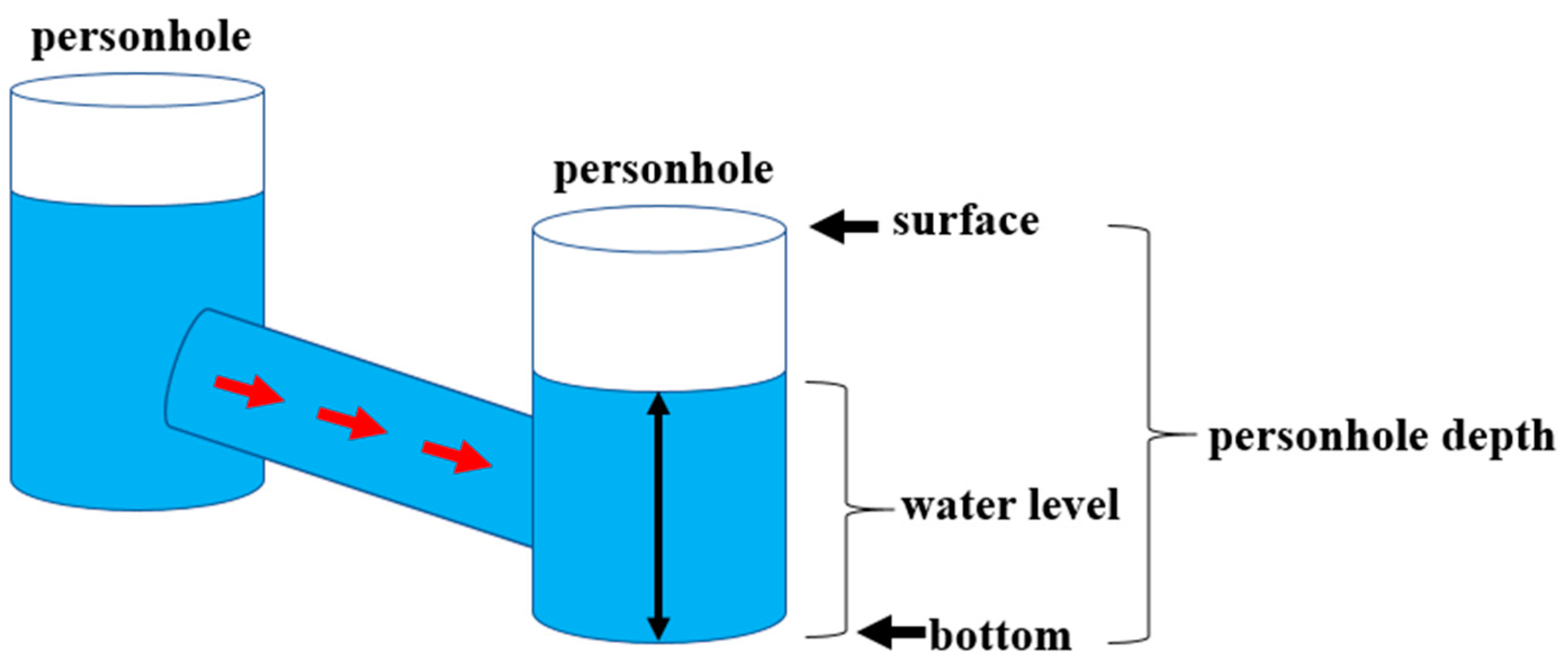Since many people work or live in the city, urban stormwater drainage systems are specifically constructed to collect and discharge precipitation to prevent water from accumulating in the city [3]. As depicted in Figure 1, the system consists of many personholes, which are connected by pipelines. During rainfall, water enters the system through street drains and personholes, flowing towards sewage treatment plants or directly discharging into nearby rivers or oceans. If the water level within a certain personhole exceeds its depth, the personhole will overflow and the street might be flooded. There are several challenges in stormwater management currently. Unexpected rainfall or storm surges occur frequently, with uneven distribution. Additionally, regional variations also affect how rainfall can enter the drainage system smoothly. Therefore, with the help of overflowing personhole prediction, we can estimate the degree of severity of the city flooding in a specific region more precisely.

Many efforts have been made to detect if a flood is occurring or to produce warning messages [4,5,6]. Researchers have also studied how to perform flood forecasting so that governments and residents can take action in advance to reduce the damage. The traditional way is to build mathematical models based on the hydraulic discipline [7,8,9]. However, this method requires complicated computations, which take a great deal of time, and might fail to provide an instant warning. Presently, researchers have been exploring the application of artificial intelligence (AI) technologies, particularly machine learning (ML), to address this issue [10,11]. The machine learning technique can be classified as a data-driven approach, since it requires a great deal of training data to compute the statistical relationship between the input and output data. Many models have been proposed, and one of the most common is the artificial neural network (ANN) model, which can model linear or nonlinear systems. Here, we discuss some existing research outcomes. Chang et al. applied the K-means clustering method [12] to categorize the data points of the different flooding characteristics in the study area and integrated an ANN model to propose a clustering-based hybrid inundation model (CHIM) for forecasting 1 h ahead inundation extents and depths [13]. Liu et al. integrated a back-propagation ANN model with stacked autoencoders to construct a flood forecasting model, where the latter was used to extract important features and the former was used for forecasting [14].

Instead of performing forecasting based on particular data points, some researchers studied how to create inundation maps directly [15,16]. For example, the region was first divided into 75 m × 75 m grids, and the self-organizing map (SOM) and recurrent nonlinear autoregressive with exogenous inputs (RNARX) were applied to produce regional flood inundation maps [17]. In addition, a special type of neural network that implements a memory mechanism to store important information from the previous steps, the recurrent neural network (RNN), has been applied to process time sequence data [18]. An evolution of the RNN, the long short-term memory neural network (LSTM), also attracts a great deal of attention. For example, it was used for one-day-, two-day-, and three-day-ahead flowrate forecasting at Hoa Binh Station [19] and was used for rainfall runoff modeling for flood events [20,21].

One requirement of applying the above approach is that we need a large amount of data, which might be hard to obtain. Therefore, the technique of transfer learning or fine-tuning has been proposed [22]. It involves taking a pre-trained model that has been trained on a large dataset for a specific task. This pre-trained model’s weights and architecture are then used as a starting point for training a new model on a different but related task or dataset. These techniques have been used in several areas, such as image processing [23,24,25], and are currently also applied in the hydraulic discipline. Zhao et al. pre-trained a convolutional neural network-based assessment model in one catchment and then tried to improve the model performance of two other catchments by transferring knowledge from the pre-trained model [26]. Kimura et al. investigated the transfer learning approach to reduce the training time, in which the CNN model was used as a basis for flood prediction [27].

This study explores methods to predict whether specific personholes in urban areas are likely to overflow. The considered artificial intelligence technologies include those previously mentioned, such as the ANN model, the LSTM model, and the fine-tuning technique. We propose gathering historical data regarding rainfall and water levels in personholes and utilizing this extensive data to train machine learning models for future predictions. However, several challenges exist. Firstly, there are numerous personholes in a city, so training a model for each personhole individually is time-consuming. Secondly, personholes only overflow under specific circumstances, and it is not a frequent occurrence. If each personhole is separately trained, the proper training dataset would be significantly small. Conversely, if all personholes’ data are combined to construct a single predictive model, it may not fit the conditions of each personhole. Therefore, we will initially group personholes and investigate which features are suitable for clustering. We will additionally discuss whether the fine-tuning architecture or heuristic rules could be applied to enhance performance.

2. Study Area and Data

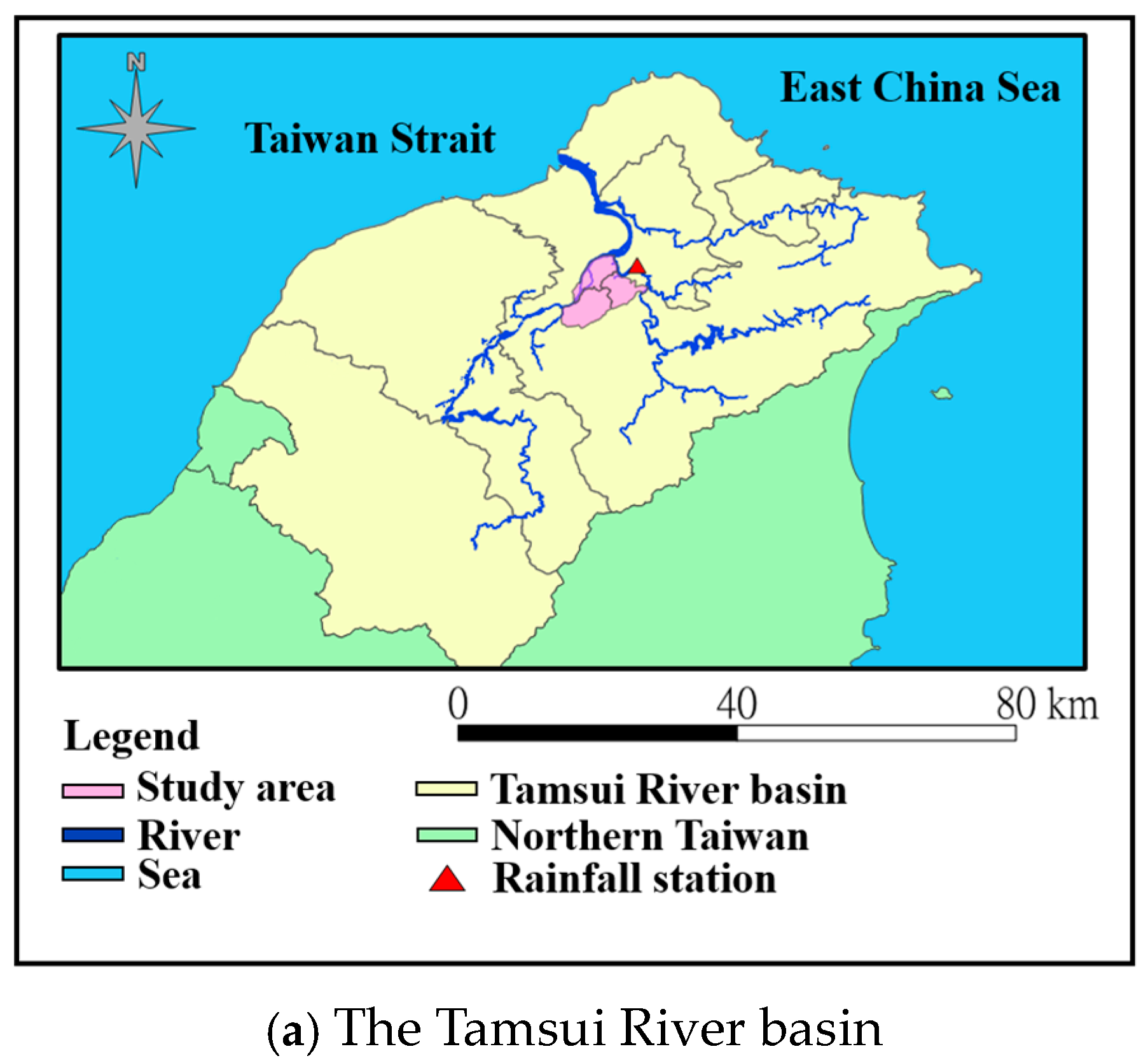
The study focuses on the downstream region of the Tamsui River. The Tamsui River basin is situated in Northern Taiwan, as illustrated in Figure 2a. This area is home to nearly 8 million people and has a developed industrial and commercial presence. The Taipei metropolitan area is also located here, serving as the political, economic, and cultural hub of Taiwan.

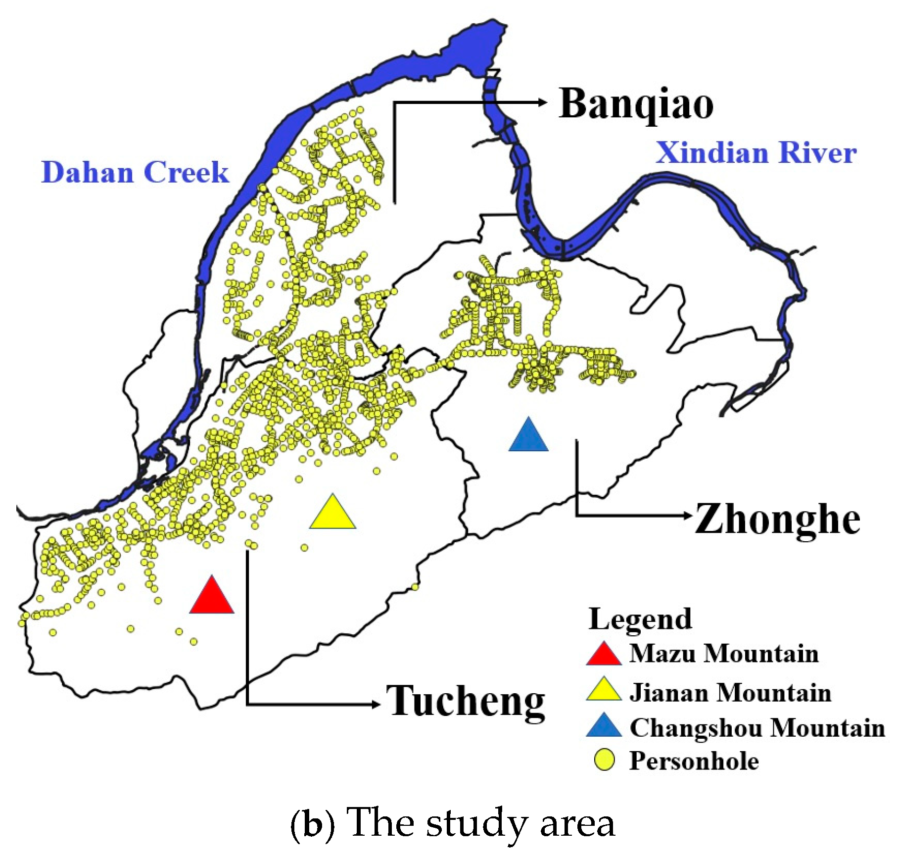
The Tamsui River has three tributaries: the Dahan Creek, the Keelung River, and the Xindian River. Among these three tributaries, the Dahan Creek and the Xindian River converge in the Banqiao District of the New Taipei City. After merging with the Keelung River, the Tamsui River flows into the Taiwan Strait. This study considers the Banqiao District along with the nearby Zhonghe and Tucheng Districts, which are part of the Taipei metropolitan area, with a total area of approximately 73 square kilometers. As depicted in Figure 2b, the research area is not only surrounded by two rivers in the northern part but also has three mountains in the southeast. Due to its unique geographic characteristics, there were frequent and severe floods in the past, and the authorities constructed stormwater drainage systems to manage street runoff. Since the personholes that are in the mountain area seldom overflow, we only focus on the personholes located in the plain. There are 2231 personholes considered in this research, and their geological locations are marked by yellow dots in Figure 2b.

To construct the ML model, we collected twenty-one events that made the personhole overflow in the study area, which might have been associated with typhoons or heavy rainstorms. As listed in

Table 1. Events of personhole overflowing in the study area.

Event No.	Type	Start	End	Duration (Hour:Minutes)
1	Typhoon	6 October 2007 00:20	7 October 2007 00:10	23:50
2	Typhoon	13 September 2008 00:20	15 September 2008 09:50	57:30
3	Typhoon	27 September 2008 01:10	30 September 2008 06:00	76:50
4	Typhoon	20 October 2010 00:40	22 October 2010 00:30	47:50
5	Rainstorm	25 June 2011 00:40	26 June 2011 17:50	41:10
6	Rainstorm	11 June 2012 22:00	12 June 2012 22:00	24 h
7	Typhoon	1 August 2012 10:10	3 August 2012 01:00	38:50
8	Typhoon	20 August 2013 04:40	22 August 2013 03:50	47:10
9	Typhoon	20 September 2013 02:50	21 September 2013 00:30	21:40
10	Rainstorm	30 June 2014 14:10	30 June 2014 18:50	4:10
11	Rainstorm	23 March 2015 07:10	23 March 2015 21:00	13:50
12	Rainstorm	4 May 2015 23:10	5 May 2015 15:50	16:40
13	Typhoon	7 August 2015 19:10	8 August 2015 14:00	18:50
14	Rainstorm	17 June 2016 14:30	17 June 2016 21:30	7 h
15	Rainstorm	29 June 2016 15:10	30 June 2016 00:50	9:40
16	Rainstorm	2 June 2017 02:55	4 June 2017 17:55	63 h
17	Rainstorm	13 June 2017 13:45	18 June 2017 19:35	125:50
18	Rainstorm	11 October 2017 00:15	15 October 2017 23:55	119:40
19	Typhoon	10 July 2018 16:05	11 July 2018 09:05	17 h
20	Rainstorm	2 July 2019 13:45	3 July 2019 06:15	16:30
21	Rainstorm	22 July 2019 07:45	22 July 2019 16:55	9:10

, the years span from 2007 to 2019. The start time, end time, and duration of each event are recorded. In this research, we required rainfall information near personholes since it is the main factor making a personhole overflow (The rainfall was measured in millimeters and the water level is in meters). The data were measured at the Zhong-Zheng Qiao rainfall station every ten minutes, which is located in the east of the study area, as shown in Figure 2a. This station was chosen since it is one of the oldest stations and can provide enough historical data. The rainfall data were purchased from the official Water Resources Agency, where all the data were verified and did not contain missing values. However, the raw data correspond to accumulated rainfalls. We converted them to the rainfall intensity in ten minutes for future use. Additionally, the water levels of personholes are also needed for the training and testing of the ML model. Since it is difficult to obtain the actual water level of all personholes for all the events, the Storm Water Management Mode (SWMM) (https://www.epa.gov/water-research/storm-water-management-model-swmm (accessed on 1 July 2020)) was applied to produce the required sequence, in which the parameters are calibrated according to the real water level. These data will be used to train and test the machine learning model.

3. Methodology

In this paper, we apply machine learning techniques to build the model for predicting if personholes will overflow soon. There are two important points worth mentioning. First, we apply a group-based method to train the model. That is, instead of training an individual model for each personhole or only a model for all personholes, we train a model for each group. We design different ways of forming groups and will investigate the performance of each approach. Second, we also try to apply the concept of the fine-tuning technique in the machine learning field to this study. Specifically, we use a pre-trained model, which was trained based on the complete personhole dataset, and we intend to let the model parameters be fine-tuned to meet the characteristics of each group. The proposed method will be explained in more detail in the following subsections.

3.1. Methods of Forming Groups

The disadvantages of building a prediction model for each personhole are twofold. First, there will be numerous models to maintain. Second, a single personhole is often not associated with numerous flooding events, thus lacking sufficient data to train a robust model. In this research, we use some representative features to run the k-means algorithm [12], which is a well-known algorithm for clustering data points, and divide all personholes into eight groups.

We propose two methods of forming groups, which correspond to two different feature sets for running the clustering algorithm. In the first method, which is also referred to as the geography-based method, we only use the locations of the personholes as the features, where the longitude and latitude represent the locations. The result of this method is shown in Figure 3.

We can see that the advantage of this approach is that all the personholes of each group are located very near. The characteristics of each group, which include the center of each group and the number of personholes within each group, are listed in

Table 2. The characteristics of the eight groups formed by the first grouping method.

ID	Center	Number of Personholes
I-1	(121.4201619, 24.96051094)	204
I-2	(121.48470371, 25.0011108)	336
I-3	(121.46247585, 24.98718612)	352
I-4	(121.45416902, 25.00497993)	245
I-5	(121.49527851, 24.99138239)	288
I-6	(121.43777793, 24.97113962)	277
I-7	(121.45808409, 25.02157685)	263
I-8	(121.4490086, 24.98721952)	266

. We can also observe that the size of each group does not vary a great deal. However, the disadvantage of this method is that the location of a personhole might not directly lead to its overflowing.

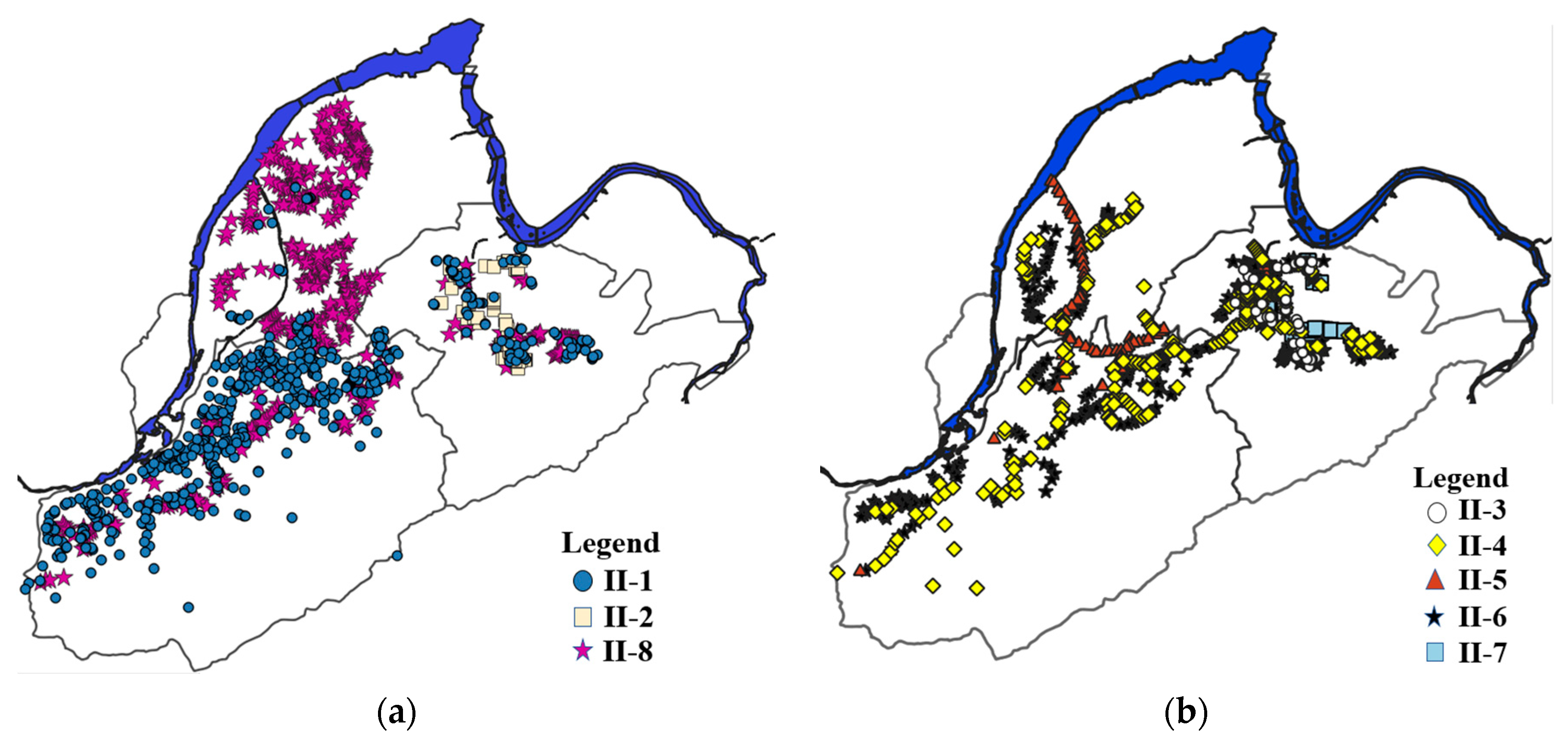
In the second method, which is referred to as the hydrology-based method, the feature sets for executing the k-means algorithm include three features directly associated with the overflowing of a personhole: the personhole depth, the average water level of the personhole, and the maximum water level of the personhole. We similarly divide all personholes into eight groups, and the results are depicted in two figures to avoid cluttering and for clearer illustration, in which the locations of the personholes within groups II-1, II-2, and II-8 are shown in Figure 4a, while the personholes of the remaining five groups are shown in Figure 4b. As can be seen, the personholes within the same group might be dispersed a great deal. We further list several characteristics of each group in

Table 3. The characteristics of the eight groups formed by the second grouping method.

ID	Avg. Personhole Depth	Avg. Water Level	Avg. Max. Water Level	Number of Personholes
II-1	4.625	0.185	1.164	280
II-2	0.1	0.084	0.344	550
II-3	0.1	6.961	8.188	49
II-4	3.507	0.420	2.152	281
II-5	5.820	0.854	3.737	102
II-6	1.804	0.728	1.854	379
II-7	0.1	3.738	5.778	30
II-8	2.391	0.058	0.325	560

. The first one is the average depth of the personholes in the group. The second is obtained by first calculating the average water level of each personhole and then calculating the group average. The third one is calculated in the same way except using the maximum value instead of the average value of each personhole. The number of personholes is also shown in the last column of the table for comparison. We can see that all the characteristics vary a great deal among the groups.

3.2. Basic Forecasting Models

We intend to build a model based on machine learning techniques to predict if a personhole will overflow soon. The features include the amount of rain that fell every ten minutes and the rainfall total for the past three hours, since a sudden large amount of rain and the accumulated amount are the direct causes of floods. Specifically, let the current time be denoted as $t$, ten minutes after the current time as $t+1$, ten minutes before $t$ as $t-1$, etc. $R_t$ is used to represent the rainfall intensity at t, which is the cumulative rainfall from the past ten minutes to the current time. All the features used in the machine learning model are as follows and collectively denoted as ${FS}_t$:

• $R_t$, $R_{t-1}$, …, $R_{t-17}$: the rainfall intensity obtained every ten minutes for the past three hours;
• $S_t$: the sum of all the 18 rainfall intensities $R_t$, $R_{t-1}$, …, $R_{t-17}$;
• $M_t$: the maximum value among all the 18 rainfall intensity $R_t$, $R_{t-1}$, …, $R_{t-17}$.

Although the main goal is to output a Boolean value, F_t+1, to show if a personhole will overflow at $t+1$ or not, we will first predict the water level at time $t+1$, denoted as $D_{t+1}$, for two reasons. First, a personhole only overflows on some special occasions. Therefore, the situation of underflow and overflow within the dataset is not even, which is usually not suitable for training a classifier. Second, there are some advantages to predicting the water level first. For example, it can be used as a precaution if the level exceeds a predefined threshold.

We now present the prediction function for our machine learning model. Suppose a personhole belongs to the m_th group. The function f_m will output the predicted water level for each personhole i in the m_th group at t + 1 based on its corresponding feature set FS_t. We then predict if the personhole i will overflow by comparing D_t+1 with its own depth d_i. The complete idea is summarized by the function F as follows, where the value 0 corresponds to the underflow state and the value 1 corresponds to the overflow state:

$$F_{t+1}^i=\left\{ \begin{array}{c}0, \mathrm{if} f_m\left(F{S}_t\right)=D_{t+1}<d_i\hfill \\ 1, \mathrm{otherwise}\hfill \end{array}\right.$$

(1)

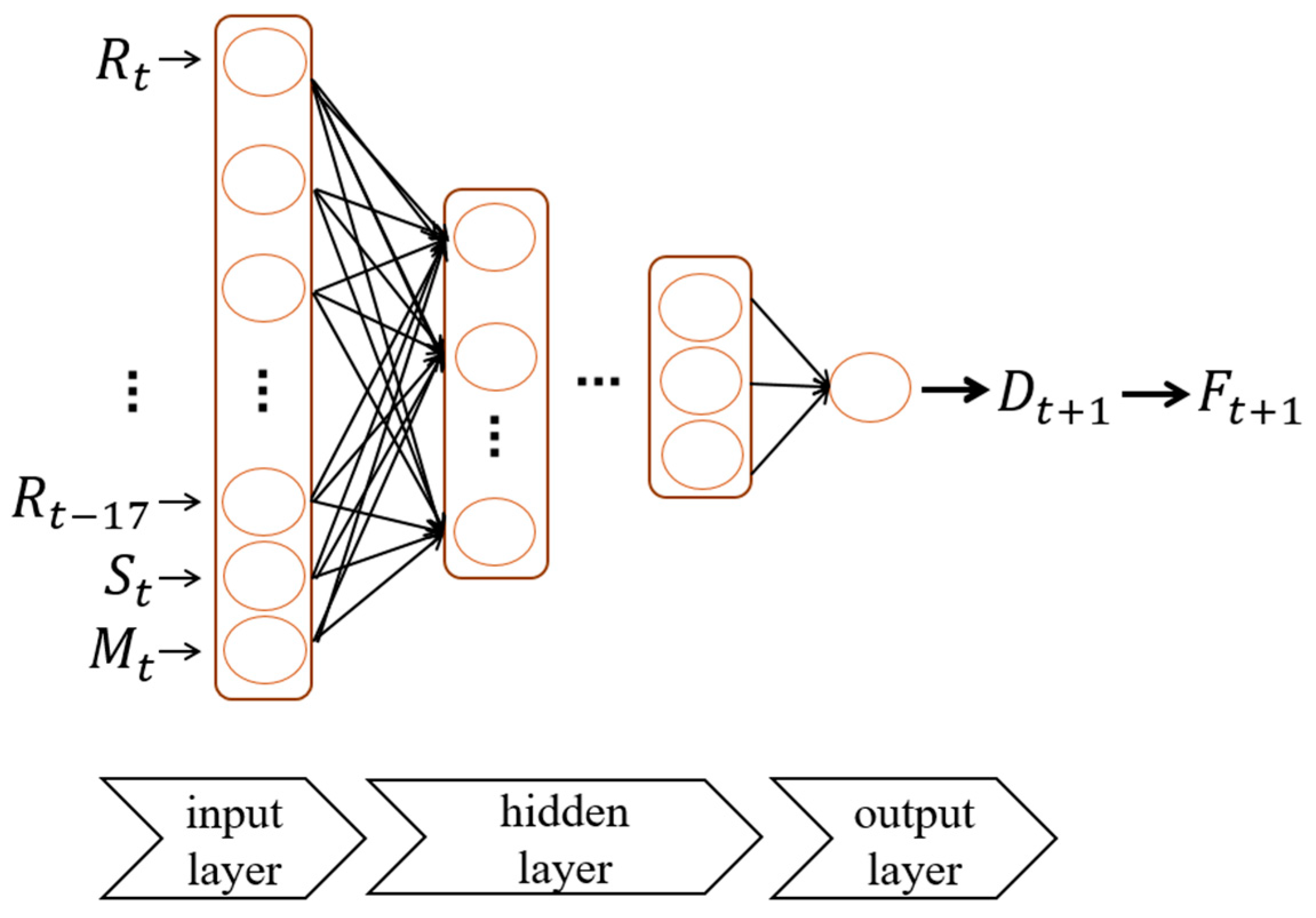
We first use the MultiLayer Perceptron (MLP) model to implement the prediction function, where an MLP is a feedforward ANN that creates outputs from a group of inputs with a back-propagation training algorithm. We chose MLP since it can be applied to complex nonlinear problems and provide quick predictions after training. It is characterized by multiple layers of nodes connected as a directed connection between the input layer, one or more hidden layers, and the output layer [28]. The corresponding architecture is depicted in Figure 5. The model used in this study consists of five layers, with the number of neutrons as 20, 10, 5, 3, and 1, respectively. In the training phase, the entries associated with a particular personhole within the same group will form a set, where each entry consists of the input features ${FS}_t$ and the actual water level ${\check{D}}_{t+1}$. In the prediction phase, the model will first compute the predicted water level $D_{t+1}$ based on the 20 input variables $R_t$, $R_{t-1}$, …, $R_{t-17}$, $S_t$, $M_t$, and then output $F_{t+1}$ according to Formula (1).

3.3. Advanced Architecture

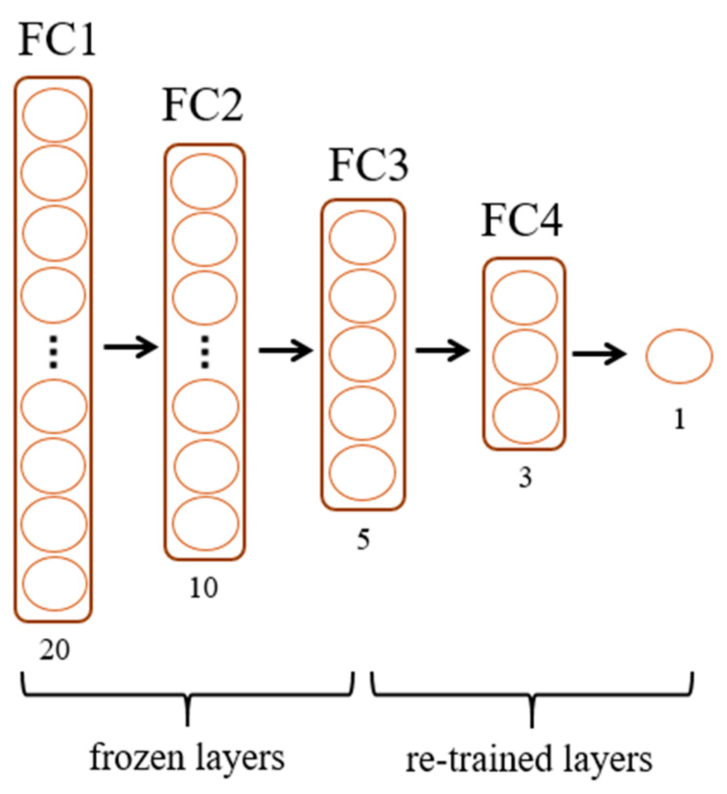
The above approach is to apply the architecture shown in Figure 5 on the dataset associated with each group of personholes separately. In this subsection, we propose two advanced architectures. First, we design a fine-tuning architecture. As shown in Figure 6, we take a pre-trained model, the architecture of which is essentially in sync with that in Figure 5, with five fully connected (FC) layers. We keep the weights of several layers in the pre-trained model, denoted as frozen layers, and re-train the model or each group of personholes. A good practice is to freeze layers from near the input to near the output, since the former captures more general features and the latter captures more specific features. Layer freezing means that the layer weights of the trained model do not change when reused on a subsequent downstream mission. In other words, when backpropagation is performed during training, these layer weights are not compromised. Such an idea is usually applied to train a different but related task, or the size of the dataset is small. In this research, since the dataset for each group of personholes is limited, we wish to explore the fine-tuning technique and will perform experiments to observe how the number of frozen layers affects the performance.

Additionally, we observe that some personholes have never overflowed. Such a situation is not good for machine learning since it requires proper datasets. On the other hand, something obvious can directly lead to the conclusion using heuristics, which is a common artificial intelligence technique. Therefore, we let UF represent the set of such kinds of personholes and directly predict that the component personhole will not overflow in any case. Otherwise, the output will be based on the result predicted by the machine learning model. This concept is described by the Formula (2), and the resultant architecture is called the mixed architecture since it can be seen as a combination of machine learning algorithms and the rule-based approach.

$$F_{t+1}^i=\left\{ \begin{array}{c}0, i\in UF \mathrm{or} f_m\left(F{S}_t\right)=D_{t+1}<d_i\hfill \\ 1, \mathrm{otherwise}\hfill \end{array}\right.$$

(2)

3.4. Evaluation Criteria

We use several metrics to evaluate the performance of the proposed prediction models, which include precision, recall, F1-score, and accuracy. Precision is the fraction of relevant instances among the retrieved instances. Recall is the fraction of relevant instances that were retrieved. Their definitions are listed in Formulas (3) and (4), where TP is shorthand for true positive, FP is shorthand for false positive, TN is shorthand for true negative, and FN is shorthand for false negative. To consider precision and recall together, a popular metric is the F1-score, as listed in Formula (5). It is also named the F-measure or F-score, and is a harmonic mean of the precision and recall [29]. Accuracy, which measures the ratio of obtaining the right prediction results, is listed in Formula (6) and is also a common metric.

$$\mathrm{p}\mathrm{r}\mathrm{e}\mathrm{c}\mathrm{i}\mathrm{s}\mathrm{i}\mathrm{o}\mathrm{n}=\frac{\mathrm{T}\mathrm{P}}{\mathrm{T}\mathrm{P}+\mathrm{F}\mathrm{P}}$$

(3)

$$\mathrm{r}\mathrm{e}\mathrm{c}\mathrm{a}\mathrm{l}\mathrm{l}=\frac{\mathrm{T}\mathrm{P}}{\mathrm{T}\mathrm{P}+\mathrm{F}\mathrm{N}}$$

(4)

$$\mathrm{F}1-\mathrm{s}\mathrm{c}\mathrm{o}\mathrm{r}\mathrm{e}=2\times \frac{\mathrm{p}\mathrm{r}\mathrm{e}\mathrm{c}\mathrm{i}\mathrm{s}\mathrm{i}\mathrm{o}\mathrm{n}\times \mathrm{r}\mathrm{e}\mathrm{c}\mathrm{a}\mathrm{l}\mathrm{l}}{\mathrm{p}\mathrm{r}\mathrm{e}\mathrm{c}\mathrm{i}\mathrm{s}\mathrm{i}\mathrm{o}\mathrm{n}+\mathrm{r}\mathrm{e}\mathrm{c}\mathrm{a}\mathrm{l}\mathrm{l}}$$

(5)

$$\mathrm{a}\mathrm{c}\mathrm{c}\mathrm{u}\mathrm{r}\mathrm{a}\mathrm{c}\mathrm{y}=\frac{\mathrm{T}\mathrm{P}+\mathrm{T}\mathrm{N}}{\mathrm{T}\mathrm{P}+\mathrm{T}\mathrm{N}+\mathrm{F}\mathrm{P}+\mathrm{F}\mathrm{N}}$$

(6)

The F1-score and accuracy will be the major metrics used in the later experiments since they can measure the prediction behavior in a more general way. For reference, we also use RMSE and SMAPE, i.e., Formulas (7) and (8), to measure the performance of predicting the water levels of personholes, in which the former measures the absolute error while the latter measures the relative or percentage error [30]. Note that $M_i$ is the actual water level, and $D_i$ is the predicted value.

Recall that we propose two grouping methods, which divide all the personholes into eight groups, respectively. Since each group performs differently, we design a weighted average, as listed in Formula (9), to reflect the performance of each grouping method as a whole. Specifically, for the i_th group, suppose the value $P_i$ represents a value computed by a certain evaluation metric and the value is not NaN (Not a Number); m_i is the number of personholes in the i_th group. The weighted average essentially considers the number of personholes in each group to compute the average, and will be used as the primary way to compare the performance of the two grouping methods.

$$\mathrm{R}\mathrm{M}\mathrm{S}\mathrm{E}=\sqrt{\frac{{\Sigma }_{i=1}^n{(M_i-D_i)}^2}{n}}$$

(7)

$$\mathrm{S}\mathrm{M}\mathrm{A}\mathrm{P}\mathrm{E}=\frac{100\%}{n}\sum _{i=1}^n\frac{\left|(D_i-M_i)\right|}{\left|D_i\right|+\left|M_i\right|}$$

(8)

$$\mathrm{w}\mathrm{e}\mathrm{i}\mathrm{g}\mathrm{h}\mathrm{t}\mathrm{e}\mathrm{d} \mathrm{a}\mathrm{v}\mathrm{e}\mathrm{r}\mathrm{a}\mathrm{g}\mathrm{e}=\frac{{\Sigma }_{i=1}^n{P}_i\times m_i}{{\Sigma }_{i=1}^n{m}_i}$$

(9)

4. Results and Discussion

In this section, we will first discuss how we determine the setting of the basic machine learning model. Then, we will design a series of experiments to evaluate the two grouping methods and the advanced architectures. The experimental results are presented and followed by a detailed discussion.

4.1. Model Setting

We apply the historical data for all personholes to train and test the basic machine learning model. Among all the events listed in Table 1, No. 1 to No. 17 are used for training, and No. 18 to No. 21 are used for testing. The size of the training dataset is 8,586,504, and the size of the testing dataset is 2,182,896, in which the size ratio between the former and the latter is about 80% to 20%. Regarding the hyperparameters, we fixed the number of epochs at 10 instead of a larger number because the dataset is quite large and we think this is enough to obtain good results. The setting of other hyperparameters followed the common practice, in which the batch size is 1000, the learning rate is 0.001, and the optimizer is Adam. Additionally, since the range of the rainfall intensity and the accumulated rainfall differ greatly, they will be normalized based on the min–max rule to the range 0–1 first, and the result will be denormalized.

Since activation functions are used to capture the linear/non-linear phenomenon of a problem domain, we wish to determine which activation function should be used in the proposed MLP model. We chose six representative activation functions to conduct empirical studies, which are listed in Formulas (10)–(15). Specifically, a sigmoid function is a mathematical function having a characteristic S-shaped curve or sigmoid curve and the logistic function is commonly used [31]. tanh is one of the hyperbolic functions and softsign is an alternative. ReLU (rectified linear unit) is the positive part of its argument [32], and softplus can be seen as the smoothness of ReLU. ELU, the exponential linear unit, speeds up learning and alleviates the vanishing gradient problem via the identity of positive values [33].

$$sigmoid(x)=\frac{1}{1+e^{-x}}$$

(10)

$$tanh\left(x\right)=\frac{\mathit{sinh}x}{\mathit{cosh}x}=\frac{e^x-e^{-x}}{e^x+e^{-x}}$$

(11)

$$softsign\left(x\right)=\frac{x}{1+\left|x\right|}$$

(12)

$$softplus\left(x\right)=\mathit{log}(1+e^x)$$

(13)

$$ELU\left(x\right)=\left\{ \begin{array}{c}\hfill x, \mathrm{if} x>0\\ \hfill \alpha \times (\mathit{exp}\left(x\right)-1), \mathrm{if} x\le 0\end{array}\right.$$

(14)

$$ReLU\left(x\right)=max(0,x)$$

(15)

Recall that the F1-score and accuracy are related to overflow prediction, and when the value is higher, the better, while RMSE and SMAPE measure the error of the predicted water level, and when the value is lower, the better. As shown in

Table 4. Performance comparison among six activation functions.

Function	F1-Score	Accuracy	RMSE	SMAPE
sigmoid	0.871	0.935	1.478	54%
tanh	0.879	0.938	1.464	53%
softsign	0.858	0.937	1.489	54%
softplus	0.875	0.933	1.474	54%
ELU	0.880	0.939	1.470	53%
ReLU	0.881	0.939	1.468	53%

, the functions tanh, ELU, and ReLU are the best three for all the four metrics. Since the last two functions are quite similar, we will apply the activation function tanh and ReLU in the subsequent experiments for comparison.

In addition, since the LSTM model is a popular model for time sequence data, we performed an empirical study to compare the performance of MLP and LSTM based on the same setting as above to determine the best machine learning model for our problem domain. As listed in

Table 5. Comparison between the MLP model and the LSTM model.

Model	Function	F1-Score	Accuracy	RMSE	SMAPE
MLP	tanh	0.879	0.938	1.464	53%
	ReLU	0.881	0.939	1.468	53%
LSTM	tanh	0.847	0.921	3.159	54%
	ReLU	0.844	0.919	3.156	54%

, the performance of LSTM is inferior to MLP for all the metrics, no matter which activation function is used, so we will use the MLP model as shown in figure hereafter. The trained model based on this architecture and the above setting will also serve as the pre-trained model in the fine-tuning architecture, as shown in Figure 6.

4.2. Analysis of the First Grouping Method

In this subsection, we analyze the performance of the first grouping method, which is also named the geography-based method, since the clustering algorithm is performed only based on the positions of personholes. The locations and characteristics of the resultant eight groups have been shown and listed in Figure 3 and Table 2, respectively. We construct a prediction model for each group individually based on the architecture shown in Figure 5 and the same setting as described in Section 4.1.

The performance of each group is summarized and listed in

Table 6. The summary of the experimental results associated with each group formed by the first grouping method.

Group	Function	F1-Score	Accuracy	RMSE	SMAPE
I-1	tanh	0.787	0.821	0.711	52%
	ReLU	0.785	0.822	0.697	52%
I-2	tanh	0.786	0.876	2.060	41%
	ReLU	0.724	0.890	2.019	41%
I-3	tanh	0.859	0.931	0.950	50%
	ReLU	0.880	0.935	0.914	50%
I-4	tanh	NaN	0.956	1.188	67%
	ReLU	NaN	0.956	1.188	67%
I-5	tanh	0.786	0.872	2.215	48%
	ReLU	0.777	0.918	2.211	56%
I-6	tanh	0.912	0.925	0.598	45%
	ReLU	0.907	0.923	0.583	44%
I-7	tanh	NaN	1	0.882	83%
	ReLU	NaN	1	0.863	80%
I-8	tanh	0.899	0.919	0.972	42%
	ReLU	0.893	0.915	0.969	42%
	weighted tanh	0.739	0.914	1.236	53%
	weighted ReLU	0.731	0.922	1.217	53%

. For each group, we show the activation function applied and the corresponding values for the four metrics. First, analyze the performance of predicting the overflow based on the F1-score and accuracy. Note that groups I-4 and I-7 have the F-1 value as “NaN”. The reason for this is that there are few or even no overflow records in the training and testing datasets, which makes the precision and recall 0 and in turn makes the denominator of Formula (5) 0. This leads to the value “NaN”. However, these two groups have the best accuracy since the model correctly determines that no overflow will occur in most cases. Note that a common way to deal with imbalanced data is to apply the over-sampling technique such as Smote [34], which improves the classification performance in certain applications [35]. However, including artificial data might affect other metrics. Therefore, we use the original dataset in this research.

Next, we analyze the performance of predicting the water level according to the values shown in the last two columns. As can be seen, the metrics RMSE and SMAPE might reveal different results for the same group, since the former measures the real differences and the latter measures the relative differences. For example, group I-1 performs best in RMSE but is not well in SMAPE. However, SMAPE seems to be the more appropriate metric in our setting since the depth of each personhole is not the same. Additionally, note that the value of RMSE is not in sync with either the value of the F1-score or accuracy. Therefore, in some experiments, we will mainly show accuracy and SMAPE to fairly evaluate the performance from different aspects. The F1-score is sometimes omitted to avoid the influence of NaN values.

As for the two activation functions tanh and ReLU, their performances also differ among groups. For example, comparing the accuracy value, I-2 is better when using ReLU while I-6 is better when using tanh. Therefore, we compute the weighted average based on Formula (9), as the last two rows show. Observe that the two activation functions excel in different evaluation criteria. Specifically, tanh is better with the F1-score while ReLU is better in accuracy and RMSE. However, the difference is not very obvious.

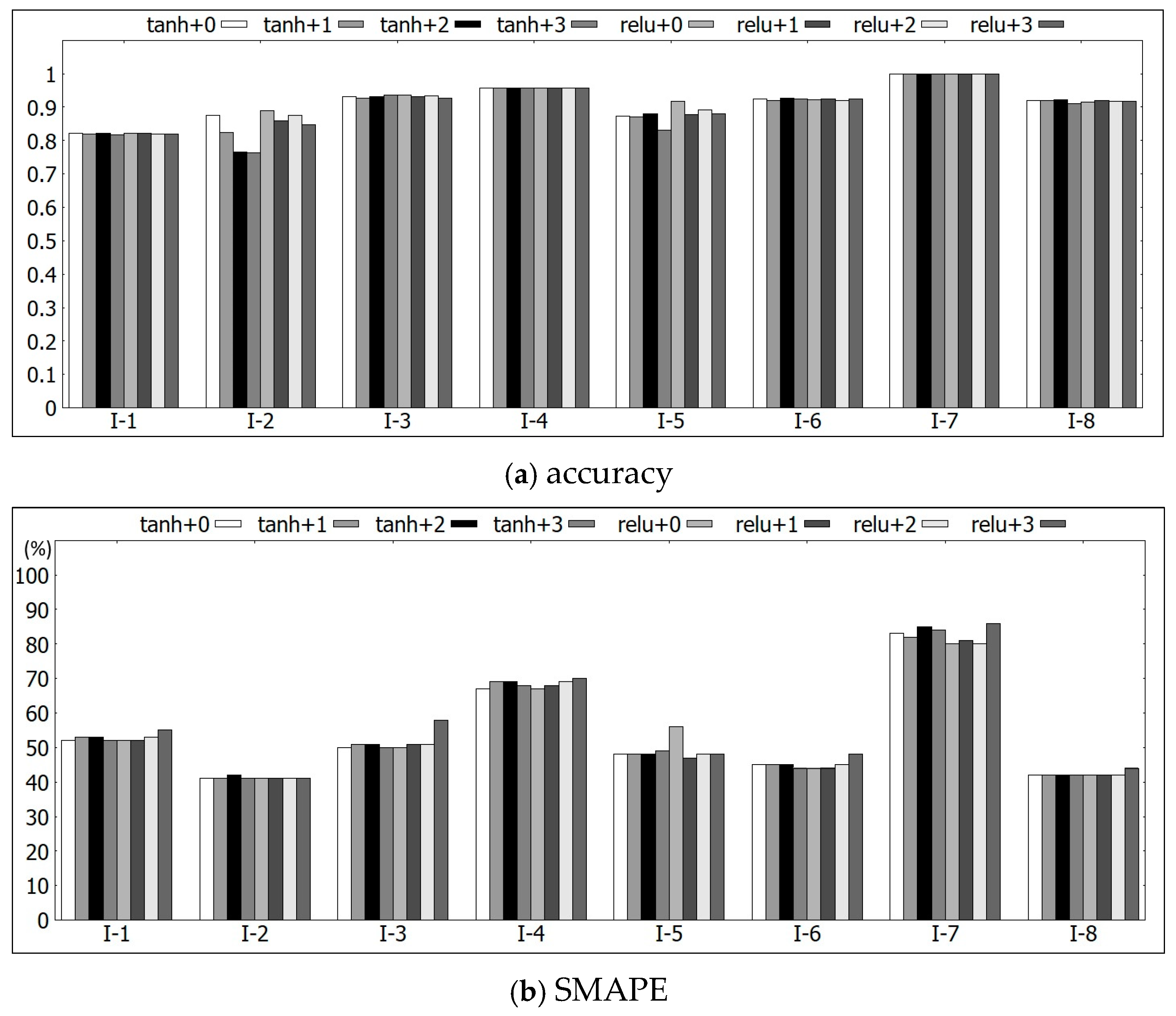
Finally, we analyze the performance of the fine-tuning architecture, which is depicted in Figure 6, based on the eight groups formed by this grouping method. The accuracy value of each group is shown in Figure 7a. In this figure, the notation “+0” means that the model is totally retrained, so the value is the same as that in Table 6; “+1” means that the set of weights between the input layer FC1 and the first hidden layer FC2 are frozen and re-used, while other layers are re-trained, etc. We also distinguish the results of applying the activation functions tanh and ReLU for comparison. Based on the experimental results, most groups do not differ a great deal among the different methods except groups I-2 and I-5. For these two groups, ReLU seems better, and using the pre-trained model with more frozen layers has a worse performance. On the other hand, the SMAPE value of each group is depicted in Figure 7b, where smaller values are better in contrast. Observe that fine-tuning some sets of weights for group I-5 indeed improves performance. However, for many other groups, such as groups I-1, I-3, I-4, I-6, and I-7, re-training does not have benefits, especially when the activation function ReLU is applied.

In summary, for the first grouping method, we observed that some geographically near groups might have similar performance in some cases. Specifically, the two groups located in Banqiao, groups I-4 and I-7, both have good accuracy but bad SMAPE. Additionally, the two groups located in Zhonghe, groups I-2 and I-5, both have good SMAPE and average accuracy. Since the model for each group is mainly determined by the data of each group, this phenomenon for these two districts should be due to the similar distribution of overflowing records in different groups within the same district. However, for activation functions and the fine-tuning architecture, the impact varies for different groups. Therefore, there is no obvious conclusion what the best setting for each district should be.

4.3. Analysis of the Second Grouping Method

In this section, we compare the performance of each group formed by the second grouping method, which is also named the hydrology-based method due to the features used to run the clustering algorithm directly linking to the overflowing state. The experimental results are summarized and listed in

Table 7. The summary of the experimental results associated with each group formed by the second grouping method.

Group	Activation function	F1-Score	Accuracy	RMSE	SMAPE
II-1	tanh	NaN	1	0.581	39%
	ReLU	NaN	1	0.555	37%
II-2	tanh	0.842	0.748	0.302	51%
	ReLU	0.831	0.749	0.288	50%
II-3	tanh	0.995	0.991	2.117	12%
	ReLU	0.995	0.991	2.047	12%
II-4	tanh	NaN	0.993	0.958	32%
	ReLU	NaN	0.993	0.690	25%
II-5	tanh	nan	0.918	0.981	22%
	ReLU	0.004	0.918	0.879	20%
II-6	tanh	0.336	0.937	0.718	32%
	ReLU	0.381	0.923	0.586	26%
II-7	tanh	0.995	0.990	1.547	15%
	ReLU	0.995	0.990	1.336	13%
II-8	tanh	NaN	1	0.327	66%
	ReLU	NaN	1	0.326	66%
	weighted tanh	0.462	0.922	0.584	45%
	weighted ReLU	0.654	0.920	0.512	42%

. Note that II-2 has the worst accuracy and the second worst SMAPE. Referring to Table 3, this group has the lowest average personhole depth and the second lowest average water level. Small differences between the predicted values and actual values can have a large impact and result in bad performance.

Compared with the result of the first grouping method listed in Table 6, more groups have the value NaN for the F1-score due to the few overflow records in that group, while a few more groups achieve the best accuracy. Since the performance of each group again differs a great deal, we compare the performance of the two grouping methods based on the weighted metrics, which are listed in the last two rows of Table 6 and Table 7. We can see that the first grouping method is better in the F1-score for both activation functions. The reason for this is that there are many NaN values when using the second grouping method. As for accuracy, the second method is better when using tanh, but the difference is not obvious. In contrast, regarding the prediction of the water level, the second grouping method is superior in both RMSE and SMAPE. Particularly, SMAPE is reduced from 53% to 42% while using the activation function ReLU and improves by more than 20%.

We also performed empirical studies to evaluate how the fine-tuning model works for the second grouping method. As depicted in Figure 8a, it does not improve the accuracy for most groups and even worsens the performance for group II-6 a great deal. As for the SMAPE value depicted in Figure 8b, the performance varies. Comparing the two activation functions, fine-tuning seems better when using tanh for groups II-1, II-4, II-6, and II-8, but worse when using ReLU for groups II-1, II-5, and II-7. Since the performance of each group varies a great deal, we again computed the weighted accuracy based on Figure 7 and Figure 8 and list the results in

Table 8. Analysis of the effect of the number of frozen layers based on the weighted accuracy.

# of Frozen Layers	0		1		2		3
activation function	tanh	ReLU	tanh	ReLU	tanh	ReLU	tanh	ReLU
first method	0.914	0.922	0.905	0.912	0.899	0.916	0.891	0.909
second method	0.922	0.920	0.922	0.921	0.864	0.919	0.914	0.921

. The best two accuracy values are marked in boldface for comparison. From the table, we can see that the best performance occurs in tanh+0, ReLU+0, and tanh+1 among the two grouping methods. Additionally, we can also see that both activation functions have the best or the second-best performance in freezing one level. Therefore, we will use the setting tanh+1 to perform the next experiment.

4.4. Analysis of the Mixed Architecture

Refer to Figure 7a and Figure 8a. Observe that the eight groups formed by the first grouping method have an accuracy ranging roughly from 0.8 to 0.9, and the difference is not much. In contrast, most of the groups formed by the second grouping method have a higher accuracy, ranging from 0.9 to 1, except that group II-2 has the worst performance. 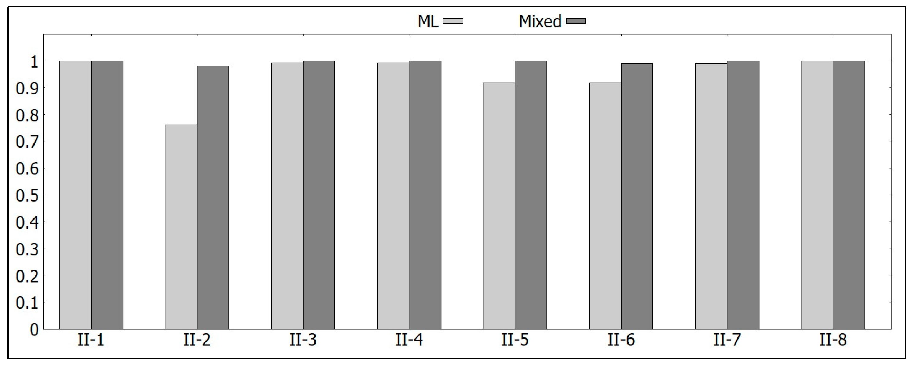Therefore, we apply the second grouping to the mixed architecture discussed in Section 3.3 to see if the performance of group II-2 can improve, in which Formula (2) is used to determine if a personhole overflows not only using the machine learning model but also based on its history. The experimental results are shown in Figure 9, in which the accuracy values based on the pure machine learning model (denoted as ML) and this mixed model (denoted as Mixed) are depicted together for comparison. Note that the group II-2 indeed reveals significant improvement. Additionally, the performances of II-5 and II-6 are also better.

To better understand the degree of improvement, the exact figures are listed in

Table 9. Performance comparison of the mixed architecture and the previous ML architecture according to the weighted average of accuracy.

	II-1	II-2	II-3	II-4	II-5	II-6	II-7	II-8	Weighted Avg.
ML	1	0.760	0.991	0.993	0.918	0.917	0.990	1	0.922
Mixed	1	0.980	1	0.999	0.999	0.989	1	1	0.993

. We can see that many groups have perfect accuracy values, and the weighted average achieves 0.993.

5. Conclusions

Flood forecasting is an important issue in real life. In this research, we considered how to predict the overflowing of personholes, which are part of an urban stormwater drainage system, based on the machine learning technique. The study area is located in the northern part of Taiwan, including the three districts Banqiao, Zhonghe, and Tucheng, and is surrounded by rivers and mountains.

An important issue that needs to be addressed in this research is how to construct a good prediction model. The basic model we used is based on the MLP model, since LSTM does not perform better in this study according to the experimental results. We also tried to identify good parameters for the MLP model, and six activation functions are specifically compared. We find that the nonlinear function tanh and the linear function ReLU are the best two representative functions, and they have their own merits among all the extensive studies. We also built a fine-tuning architecture upon the basic MLP model and investigated if there is a best setting for the number of frozen layers. However, we could only observe that it indeed affects the performance, but different groups reveal different results. Therefore, for the activation function and the number of frozen layers in the fine-tuning architecture, we can only say that using the tanh function with one frozen layer is good in some cases, but we cannot directly recommend the single best one applicable to all environments. We suggest that the readers perform empirical studies to choose the best setting in their own environment.

Another major challenge is related to the characteristics of the dataset, and two things need to be considered. First, there are thousands of personholes to predict. It will be cumbersome to maintain a prediction model for each personhole individually. Second, in the dataset used to train the machine learning model, the portion of overflowing records is very small, which is not good for building classifiers. To tackle the above-mentioned problems, we clustered all the personholes into eight groups, and two grouping methods are proposed and investigated in this paper. The first, the geography-based method, uses the geographical locations of the personholes for the grouping. The second, the hydrology-based method, uses the characteristics that are directly related to the overflowing situation, such as the depth of the personhole, and the average and maximum water level of the personholes, as the basis for grouping. For the first grouping method, the sizes of the eight groups are similar and the nearby personholes are within the same group, so the visual display effect is better. The performance of the eight groups is also similar but average. In contrast, for the second grouping method, the personholes within the same group are scattered in different places. The sizes and the performance of the eight groups vary obviously. However, using careful design, it may lead to better performance. These two methods have their own advantages and disadvantages. The choice is left to the readers.

We also analyzed the performance of the mixed architecture, which combines the result of the machine learning model and a heuristic rule based on the overflowing history of each individual group. We applied the eight groups formed by the second grouping method, mainly because group II-2 has the worst performance. The experimental results show that this indeed improves the prediction result, and the weighted accuracy involving all eight groups is almost one. Similar results were reported in [36,37], indicating that the integration of wavelet-based machine learning models significantly enhances the performance of standalone models. This shows the significance of the hybrid methods.

Overall, the experimental results have demonstrated the effectiveness and good performance of the proposed methodology, but there are several points that need to be considered for further improvement, including more features or more models, as discussed below.

First, in this paper, we exclusively employed numerical data for prediction. However, there is a trend towards integrating other types of data. For instance, Bolick et al. used the Prophet time series machine learning algorithm to predict the hourly water level variations at certain sites in urban streams. They further gathered ground optical remote sensing (lidar) data for Hunnicutt Creek, modeling these regions in 3D to elucidate how the predicted water level changes correspond to the variations in water levels within the stream channel [38]. A more comprehensive overview on the recent applications of radar data in rainfall prediction and real-time forecasting systems can be found in [39]. Additionally, since water flows in a pipeline constructed under the earth, the correspondence between the overflowing of personholes and terrain is not obvious, and is hence not considered in this research. However, this information might still affect the prediction performance and is worth considering.

Second, the AI techniques used in this paper include the MLP model, the LSTM model, the fine-tuning architecture, and heuristic rules. There are other machine learning models that can be explored. Additionally, how the transfer learning technique can be applied to predict other areas is also an interesting research issue. All the above are worthy of future research.