
Identification of Breaches in a Regional Confining Unit Using Electrical Resistivity Methods in Southwestern Tennessee, USA


Abstract
1. Introduction
2. Materials and Methods
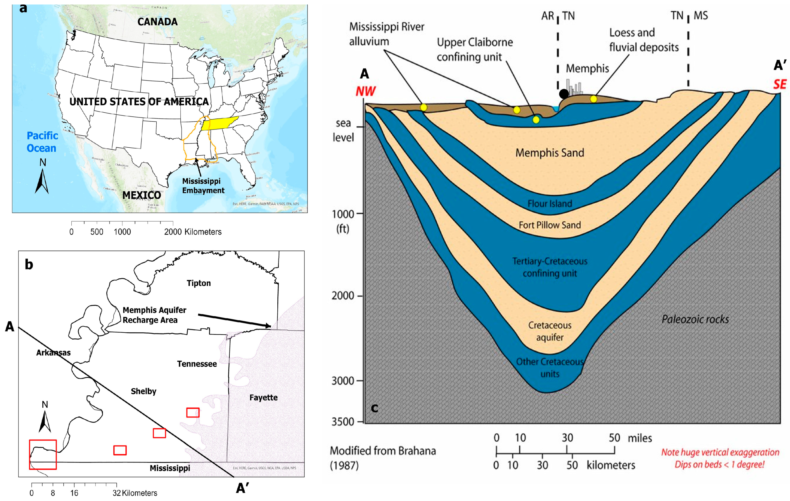
2.1. Geologic and Hydrogeologic Settings

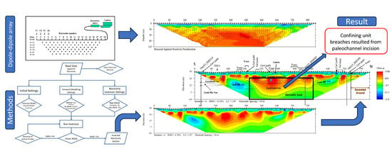
2.2. Methodology
2.2.1. Subsurface Electrical Resistivity
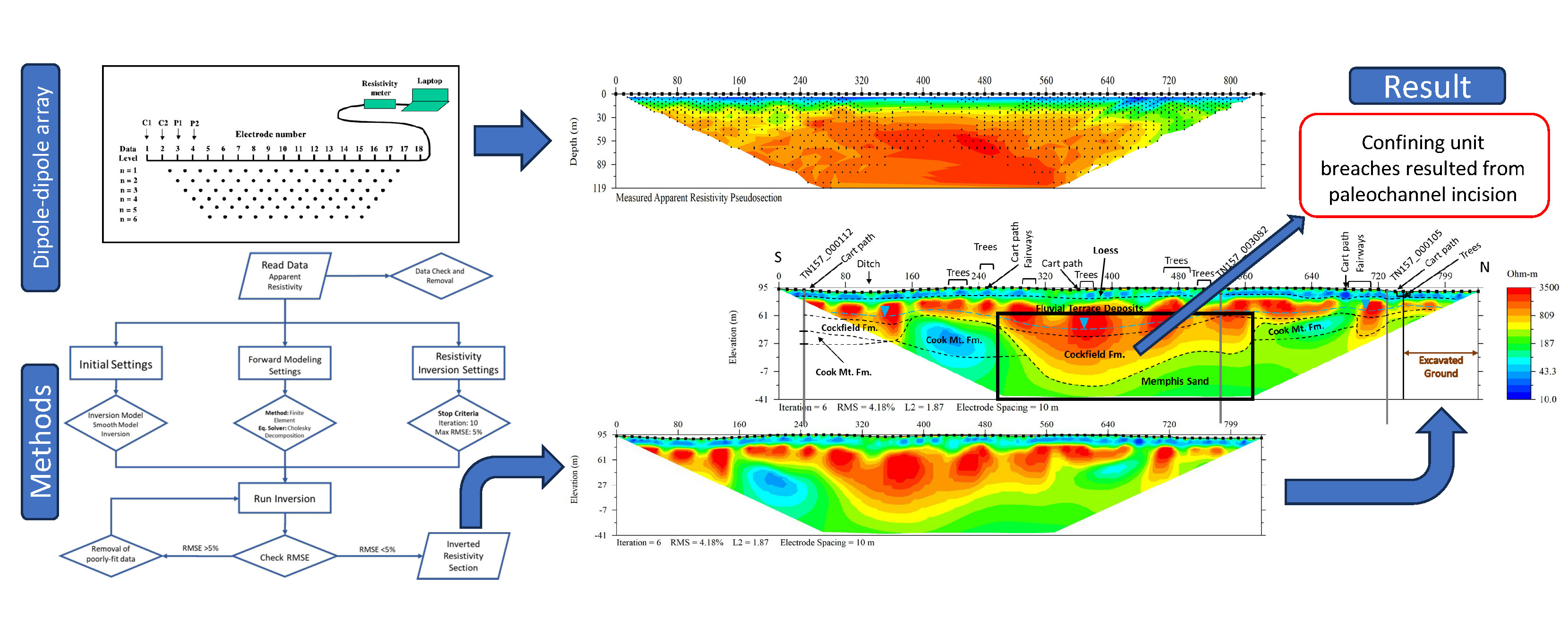
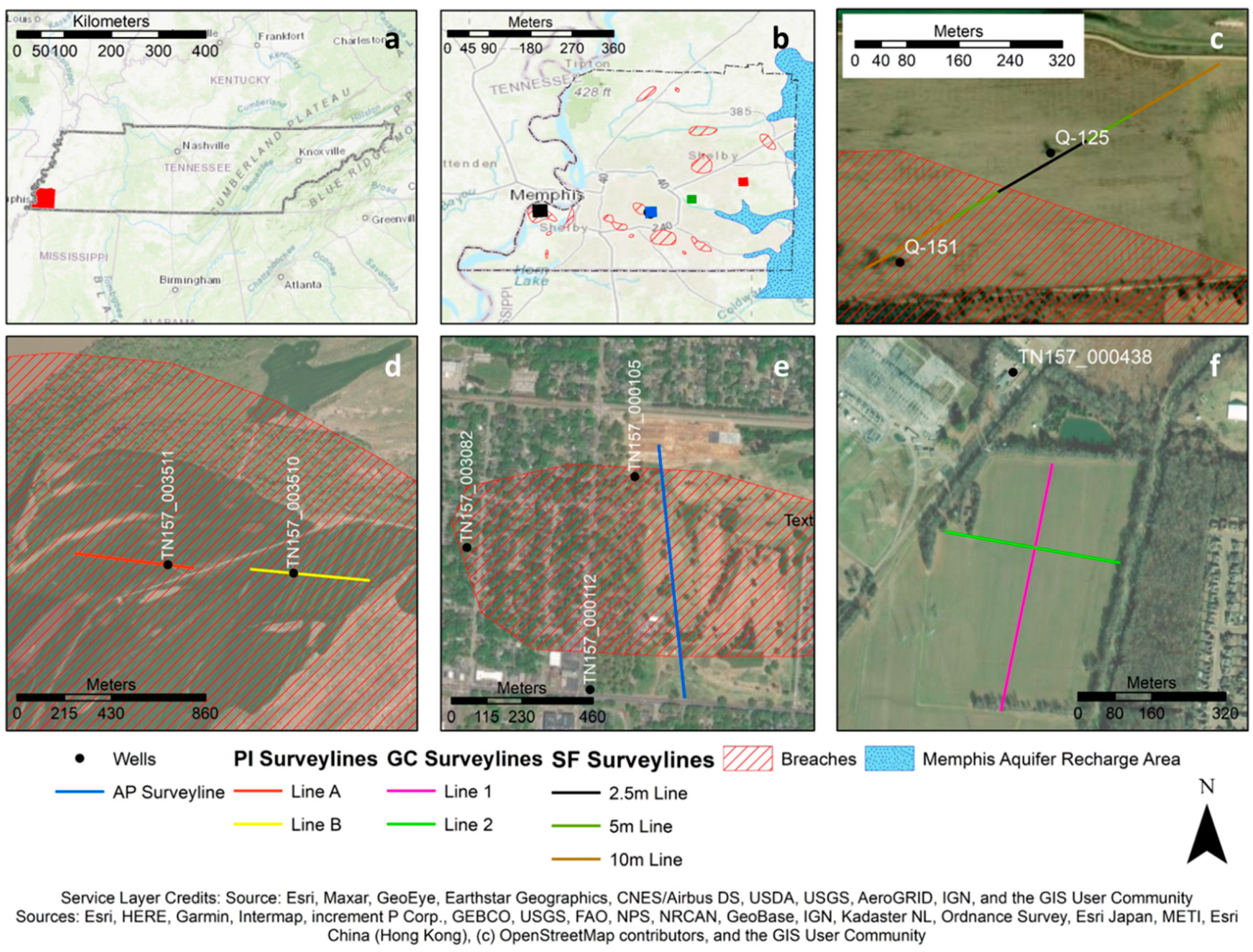
2.2.2. Data Collection
2.2.3. Array Selection and Electrode Spacing
2.2.4. Data Processing
2.2.5. Data Interpretation
3. Results
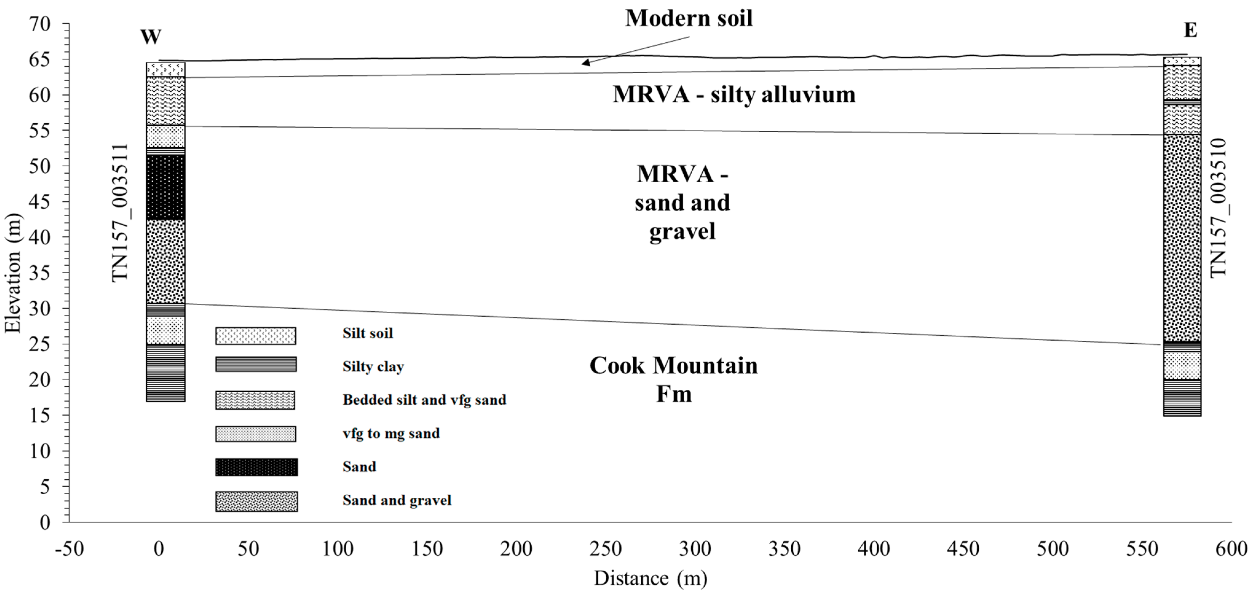
3.1. Shelby Farms
3.2. Grays Creek
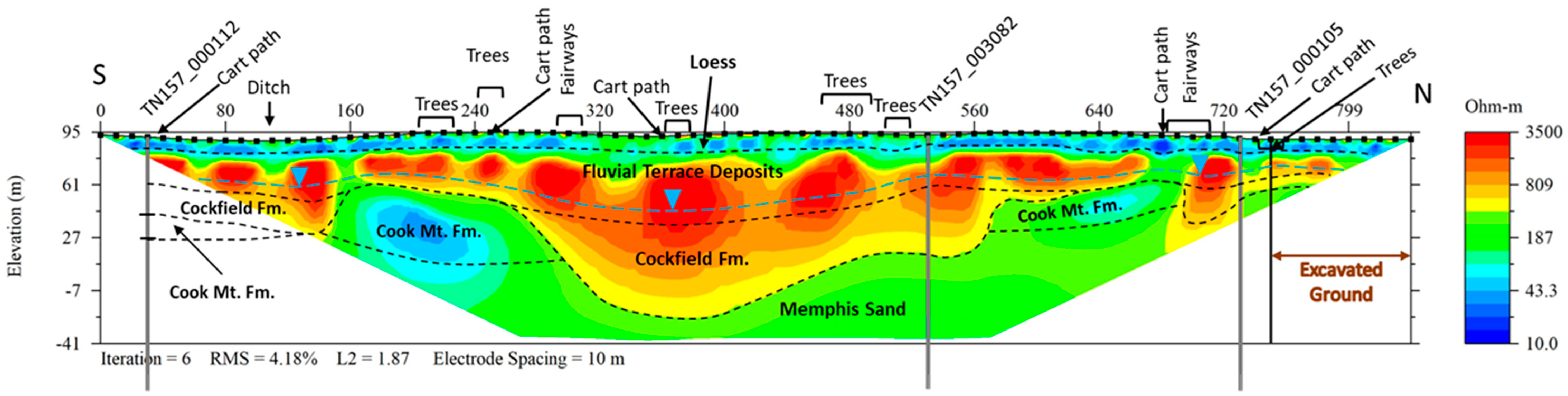
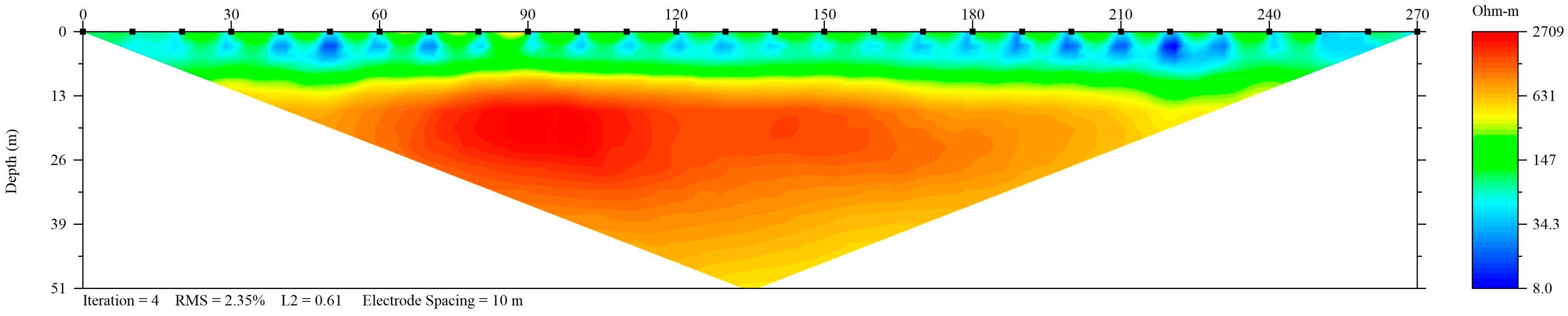
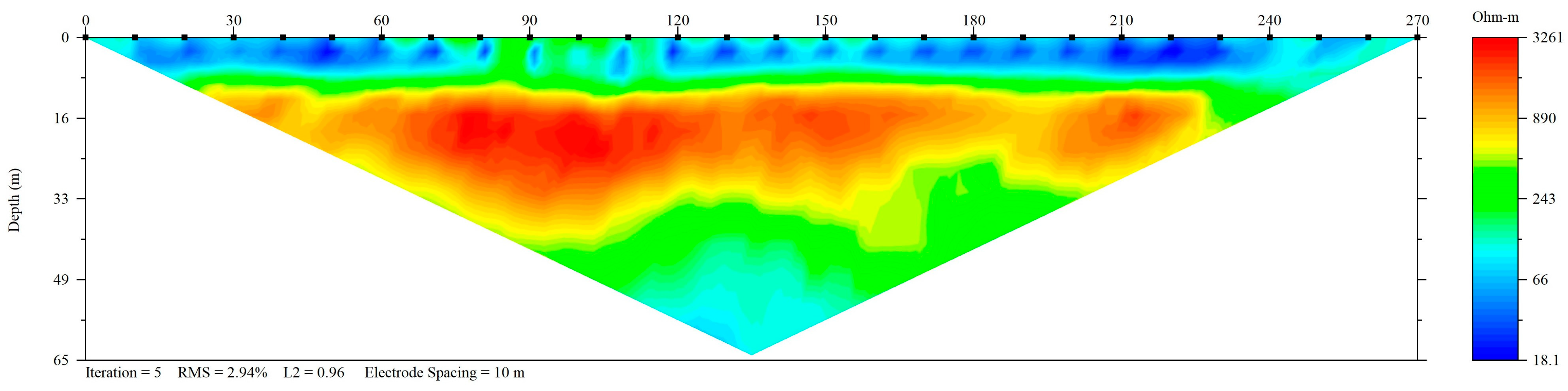
3.3. President’s Island
3.4. Audubon Park
4. Discussion
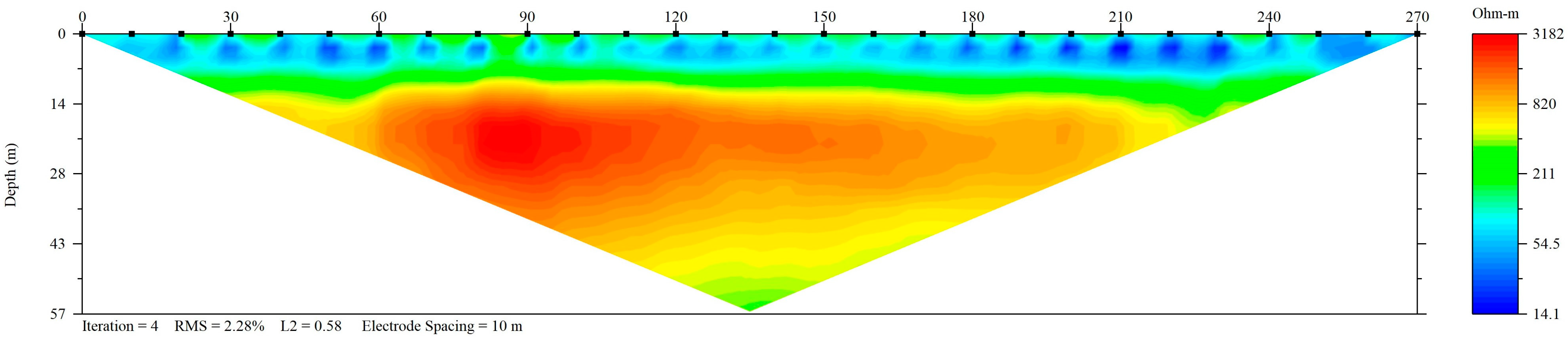
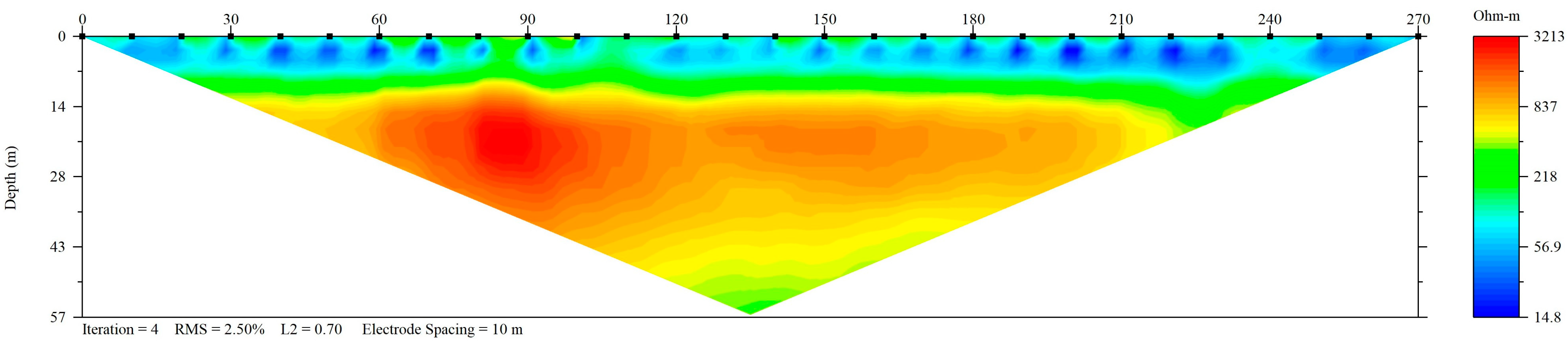
4.1. Effect of Electrode Spacing
4.2. Electrical Resistivity Data Analysis
5. Conclusions
Author Contributions
Funding
Data Availability Statement
Acknowledgments
Conflicts of Interest
Appendix A. Comparison of the Inverted Resistivity Profiles of the Data Collected Using Different Arrays


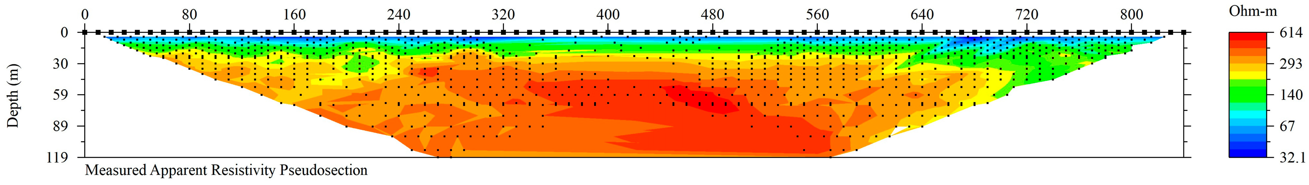
Appendix B. Apparent Resistivity Data Was Collected Using a Roll-Along Survey at Audubon Park (AP), Showing a Triangulated Zone of No Data

Appendix C. Verification of Maximum Depth of Investigation

| Array Length, L (m) | Depth of the Deepest Data Point, D (m) | D/L |
|---|---|---|
| 270 | 59 | 0.22 |
| 270 | 52 | 0.19 |
| 135 | 25.9 | 0.19 |
| Array Length, L (m) | Depth of the Deepest Data Point, D (m) | D/L |
|---|---|---|
| 550 | 119 | 0.22 |
| 385 | 78 | 0.20 |
| Array Length, L (m) | Depth of the Deepest Data Point, D (m) | D/L |
|---|---|---|
| 440 | 88 | 0.20 |
| 550 | 111 | 0.20 |
| 550 | 105 | 0.19 |
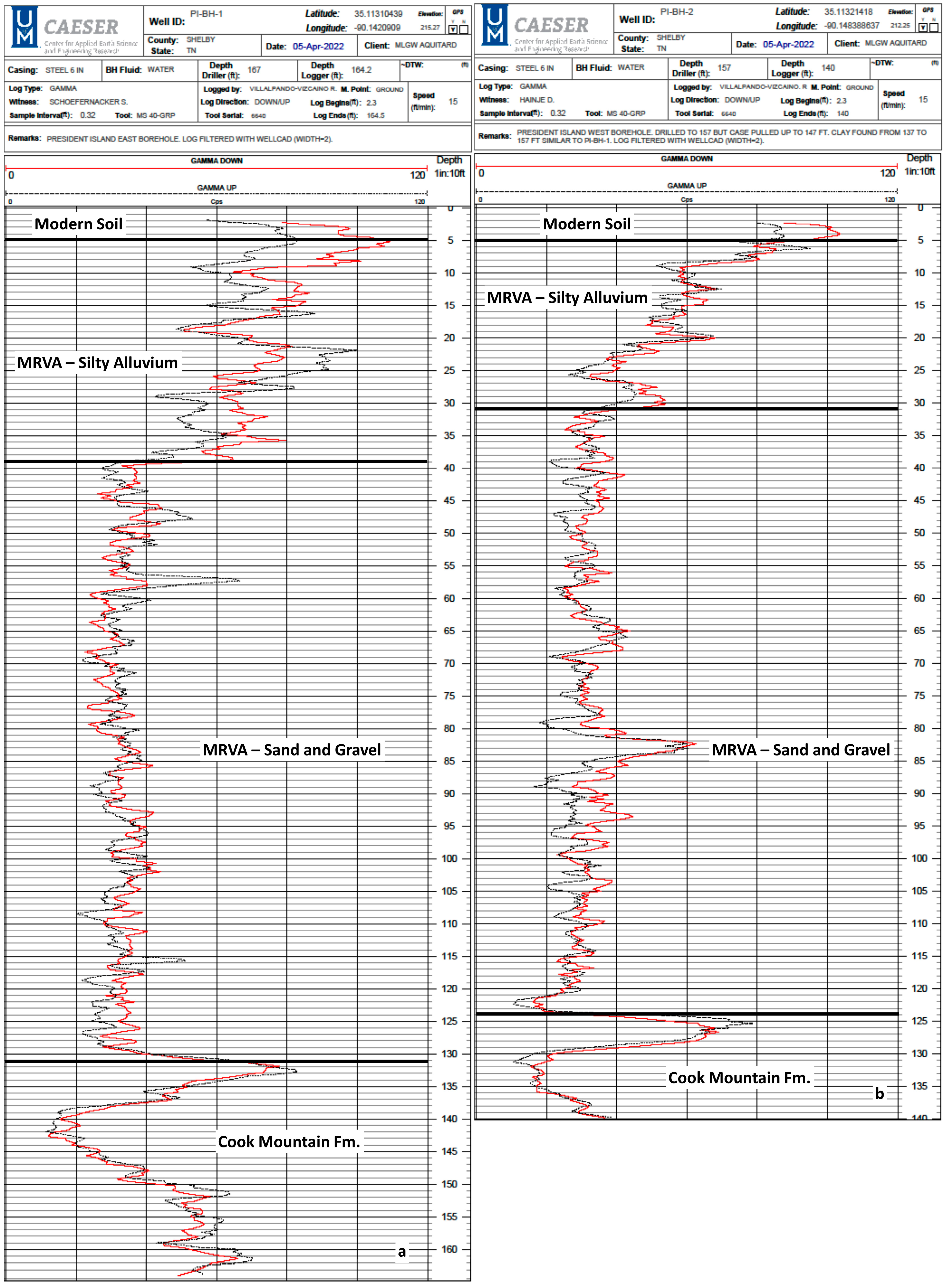
Appendix D. Gamma Logs of Boreholes Drilled at President’s Island

References
- Kowalczyk, S.; Maślakowski, M.; Tucholka, P. Determination of the Correlation between the Electrical Resistivity of Non-Cohesive Soils and the Degree of Compaction. J. Appl. Geophys. 2014, 110, 43–50. [Google Scholar] [CrossRef]
- Casagrande, M.F.S.; Furlan, L.M.; Moreira, C.A.; Rosa, F.T.G.; Rosolen, V. Non-Invasive Methods in the Identification of Hydrological Ecosystem Services of a Tropical Isolated Wetland (Brazilian Study Case). Environ. Chall. 2021, 5, 100233. [Google Scholar] [CrossRef]
- Singh, U.; Sharma, P.K. Non-Invasive Subsurface Groundwater Exploration Techniques BT—Environmental Processes and Management: Tools and Practices for Groundwater; Shukla, P., Singh, P., Singh, R.M., Eds.; Springer International Publishing: Cham, Switzerland, 2023; pp. 1–16. ISBN 978-3-031-20208-7. [Google Scholar]
- Fajana, A.O. Groundwater Aquifer Potential Using Electrical Resistivity Method and Porosity Calculation: A Case Study. NRIAG J. Astron. Geophys. 2020, 9, 168–175. [Google Scholar] [CrossRef]
- Wahab, S.; Saibi, H.; Mizunaga, H. Groundwater Aquifer Detection Using the Electrical Resistivity Method at Ito Campus, Kyushu University (Fukuoka, Japan). Geosci. Lett. 2021, 8, 15. [Google Scholar] [CrossRef]
- Wu, J.; Dai, F.; Liu, P.; Huang, Z.; Meng, L. Application of the Electrical Resistivity Tomography in Groundwater Detection on Loess Plateau. Sci. Rep. 2023, 13, 4821. [Google Scholar] [CrossRef] [PubMed]
- Schoefernacker, S. Evaluation and Evolution of a Groundwater Contaminant Plume at the Former Shelby County Landfill, Memphis, Tennessee. Ph.D. Dissertation, The University of Memphis, Memphis, TN, USA, 2018. [Google Scholar]
- Hussain, Y.; Uagoda, R.; Borges, W.; Nunes, J.; Hamza, O.; Condori, C.; Aslam, K.; Dou, J.; Cárdenas-Soto, M. The Potential Use of Geophysical Methods to Identify Cavities, Sinkholes and Pathways for Water Infiltration. Water 2020, 12, 2289. [Google Scholar] [CrossRef]
- Thomas, J.C.; Spring, M.A.; Gruhn, L.R.; Bristow, E.L. Application of Geophysical Methods to Enhance Aquifer Characterization and Groundwater-Flow. Model. Development, Des. Moines River Alluvial Aquifer, Des. Moines, Iowa, 2022; US Geological Survey: Reston, VA, USA, 2023. [CrossRef]
- Graham, D.D.; Parks, W.S. Potential for Leakage among Principal Aquifers in the Memphis Area, Tennessee; Water-Resources Investigations Report 85-4295; US Geological Survey: Reston, VA, USA, 1986. [CrossRef]
- Parks, W.S. Hydrogeology and Preliminary Assessment of the Potential for Contamination of the Memphis Aquifer in the Memphis Area, Tennessee; Water-Resources Investigations Report 90-4092; US Geological Survey: Reston, VA, USA, 1990. [CrossRef]
- Gentry, R.; McKay, L.; Thonnard, N.; Anderson, J.L.; Larsen, D.; Carmichael, J.K.; Solomon, K. Novel Techniques for Investigating Recharge to the Memphis Aquifer; American Water Works Association: Denver, CO, USA, 2006; p. 97. [Google Scholar]
- Larsen, D.; Waldron, B.; Schoefernacker, S.; Gallo, H.; Koban, J.; Bradshaw, E. Application of Environmental Tracers in the Memphis Aquifer and Implication for Sustainability of Groundwater Resources in the Memphis Metropolitan Area, Tennessee. J. Contemp. Water Res. Educ. 2016, 159, 78–104. [Google Scholar] [CrossRef]
- Carmichael, J.K.; Kingsbury, J.A.; Larsen, D.; Schoefernacker, S. Preliminary Evaluation of the Hydrogeology and Groundwater Quality of the Mississippi River Valley Alluvial Aquifer and Memphis Aquifer at the Tennessee Valley Authority Allen Power Plants, Memphis, Shelby County, Tennessee; Open-File Report 2018-1097; US Geological Survey: Reston, VA, USA, 2018.
- Larsen, D.; Waldron, B.; Schoefernacker, S. Updated Map of Semi-Confined Conditions in the Memphis Aquifer, Shelby County, Tennessee: A Work in Progress. In Proceedings of the Virtual 2022 Tennessee Water Resources Symposium, Virtual, 20–21 April 2022; TN Section AWRA: Nashville, TN, USA, 2022; p. 2C-3. [Google Scholar]
- Parks, W.S.; Carmichael, J.K. Geology and Ground-Water Resources of the Memphis Sand in Western Tennessee; Resources Investigations Report 88-4182; US Geological Survey: Reston, VA, USA, 1990. [CrossRef]
- Waldron, B.; Larsen, D.; Hannigan, R.; Csontos, R.; Anderson, J.; Dowling, C.; Bouldin, J. Mississippi Embayment Regional Ground Water Study; US Environmental Protection Agency: Washington, DC, USA, 2011; p. 192.
- Waldron, B.A.; Harris, J.B.; Larsen, D.; Pell, A. Mapping an Aquitard Breach Using Shear-Wave Seismic Reflection. Hydrogeol. J. 2009, 17, 505–517. [Google Scholar] [CrossRef]
- Larsen, D.; Schoefernacker, S.R.; Waldron, B. Stratigraphy of Upper Claiborne Strata in Western Tennessee and Hydrogeologic Implications. In Geological Society of America Abstracts with Programs 159-10; The Geological Society of America: Boulder, CO, USA, 2022; Volume 54. [Google Scholar] [CrossRef]
- Hong-Jing, J.; Shun-Qun, L.; Lin, L. The Relationship between the Electrical Resistivity and Saturation of Unsaturated Soil. Electron. J. Geotech. Eng. 2014, 19, 3739–3746. [Google Scholar] [CrossRef]
- Lu, Y.; Abuel-Naga, H.; Al Rashid, Q.; Hasan, M.F. Effect of Pore-Water Salinity on the Electrical Resistivity of Partially Saturated Compacted Clay Liners. Adv. Mater. Sci. Eng. 2019, 2019, 7974152. [Google Scholar] [CrossRef]
- Fatima Zohra, H.; Laredj, N.; Maliki, M.; Missoum, H.; Bendani, K. Laboratory Evaluation of Soil Geotechnical Properties via Electrical Conductivity Evaluación de Laboratorio de Las Propiedades Geotécnicas Del Suelo Mediante Conductividad Eléctrica. Rev. Fac. De Ing. 2019, 90, 101–112. [Google Scholar] [CrossRef]
- Corwin, D.L.; Yemoto, K. Salinity: Electrical Conductivity and Total Dissolved Solids. Soil. Sci. Soc. Am. J. 2020, 84, 1442–1461. [Google Scholar] [CrossRef]
- Ward, S.H. The Resistivity and Induced Polarization Methods. In Proceedings of the 1st EEGS Symposium on the Application of Geophysics to Engineering and Environmental Problems, Golden, CO, USA, 28–31 March 1988; Environment and Engineering Geophysical Society: Denver, CO, USA, 1998; pp. 109–250. [Google Scholar] [CrossRef]
- Zonge, K.; Wynn, J.; Urquhart, S. Resistivity, Induced Polarization, and Complex Resistivity. In Near-Surface Geophysics; Investigations in Geophysics; Butler, D.K., Ed.; Society of Exploration Geophysicists: Tulsa, OK, USA, 2005; pp. 265–300. ISBN 978-1-56080-130-6. [Google Scholar]
- Bedrosian, P.A.; Schamper, C.; Auken, E. A Comparison of Helicopter-Borne Electromagnetic Systems for Hydrogeologic Studies. Geophys. Prospect. 2016, 64, 192–215. [Google Scholar] [CrossRef]
- Baldridge, W.S.; Cole, G.L.; Robinson, B.A.; Jiracek, G.R. Application of Time-Domain Airborne Electromagnetic Induction to Hydrogeologic Investigations on the Pajarito Plateau, New Mexico, USA. Geophysics 2007, 72, B31–B45. [Google Scholar] [CrossRef]
- Wang, H.; Revil, A. Surface Conduction Model for Fractal Porous Media. Geophys. Res. Lett. 2020, 47, e2020GL087553. [Google Scholar] [CrossRef]
- Minsley, B.J.; Rigby, J.R.; James, S.R.; Burton, B.L.; Knierim, K.J.; Pace, M.D.M.; Bedrosian, P.A.; Kress, W.H. Airborne Geophysical Surveys of the Lower Mississippi Valley Demonstrate System-Scale Mapping of Subsurface Architecture. Commun. Earth Environ. 2021, 2, 131. [Google Scholar] [CrossRef]
- Nabi, A.; Liu, X.; Gong, Z.; Ali, A. Electrical Resistivity Imaging of Active Faults in Palaeoseismology: Case Studies from Karachi Arc, Southern Kirthar Fold Belt, Pakistan. Nriag J. Astron. Geophys. 2020, 9, 116–128. [Google Scholar] [CrossRef]
- Porras, D.; Carrasco, J.; Carrasco, P.; González, P.J. Imaging Extensional Fault Systems Using Deep Electrical Resistivity Tomography: A Case Study of the Baza Fault, Betic Cordillera, Spain. J. Appl. Geophys. 2022, 202, 104673. [Google Scholar] [CrossRef]
- Larsen, D.; Gentry, R.; Solomon, D. The Geochemistry and Mixing of Leakage in a Semi-Confined Aquifer at a Municipal Well Field, Memphis, Tennessee, USA. Appl. Geochem. 2003, 18, 1043–1063. [Google Scholar] [CrossRef]
- Bradley, M.W. Ground-Water Hydrology and the Effects of Vertical Leakage and Leachate Migration on Ground-Water Quality near the Shelby County Landfill, Memphis, Tennessee; Water-Resources Investigations Report 90-4075; US Geological Survey: Reston, VA, USA, 1991; p. 47. [CrossRef]
- Parks, W.S.; Mirecki, J.E. Hydrogeology, Ground-Water Quality, and Potential for Water-Supply Contamination near the Shelby County Landfill in Memphis, Tennessee; U.S. Geological Survey Water-Resources Investigations Report 91-4173; US Geological Survey: Reston, VA, USA, 1992; p. 79. [CrossRef]
- Clark, B.R.; Hart, R.M. The Mississippi Embayment Regional Aquifer Study (MERAS): Documentation of a Groundwater-Flow Model Constructed to Assess Water Availability in the Mississippi Embayment; Scientific Investigations Report 2009–5172; US Geological Survey: Reston, VA, USA, 2009; p. 61. [CrossRef]
- Dieter, C.A.; Maupin, M.A.; Caldwell, R.R.; Harris, M.A.; Ivahnenko, T.I.; Lovelace, J.K.; Barber, N.L.; Linsey, K.S. Estimated Use of Water in the United States in 2015; Circular 1441; US Geological Survey: Reston, VA, USA, 2018; p. 65. [CrossRef]
- Van Arsdale, R.B.; Cox, R.T. The Mississippi’s Curious Origins. Sci. Am. 2007, 296, 76B–82B. [Google Scholar] [CrossRef]
- Brahana, J.V.; Broshears, R.E. Hydrogeology and Ground-Water Flow in the Memphis and Fort Pillow Aquifers in the Memphis Area, Tennessee; Water-Resources Investigations Report 89-4131; US Geological Survey: Reston, VA, USA, 2001; p. 56. [CrossRef]
- Konduru Narsimha, V.K. Altitudes of Water Levels 2005, and Historic Water Level Change in Surficial and Memphis Aquifer, Memphis, Tennessee. Master’s Thesis, The University of Memphis, Memphis, TN, USA, 2007. [Google Scholar]
- Lloyd, O.B.; Lyke, W.L. Ground Water Atlas of the United States: Segment 10, Illinois, Indiana, Kentucky, Ohio, Tennessee; Hydrologic Atlas 730; US Geological Survey: Reston, VA, USA, 1995; p. 30. [CrossRef]
- Vanderlip, C.A.; Cox, R.T.; Larsen, D.; Mitchell, J.; Harris, J.B.; Cearley, C.S. Newly Recognized Quaternary Surface Faulting and Folding Peripheral to the New Madrid Seismic Zone, Central United States, and Implications for Restraining Bend Models of Intraplate Seismic Zones. J. Geol. 2021, 129, 77–95. [Google Scholar] [CrossRef]
- Martin, R.V.; Van Arsdale, R.B. Stratigraphy and Structure of the Eocene Memphis Sand above the Eastern Margin of the Reelfoot Rift in Tennessee, Mississippi, and Arkansas, USA. GSA Bull. 2017, 129, 970–996. [Google Scholar] [CrossRef]
- Bursi, J.B. Recharge Pathways and Mechanisms to the Memphis Aquifer. Master’s Thesis, University of Memphis, Memphis, TN, USA, 2015. [Google Scholar]
- Brahana, J.V.; Parks, W.S.; Gaydos, M.W. Quality of Water from Freshwater Aquifers and Principal Well Fields in the Memphis Area, Tennessee; Water-Resources Investigations Report 87-4052; US Geological Survey: Reston, VA, USA, 1987; p. 26. [CrossRef]
- Jamaluddin; Umar, E. Identification of Subsurface Layer with Wenner-Schlumberger Arrays Configuration Geoelectrical Method. IOP Conf. Ser. Earth Environ. Sci. 2018, 118, 12006. [Google Scholar] [CrossRef]
- Clifford, J.; Binley, A. Geophysical Characterization of Riverbed Hydrostratigraphy Using Electrical Resistance Tomography. Near Surf. Geophys. 2010, 8, 493–501. [Google Scholar] [CrossRef]
- Lowry, W.F. Geophysical Techniques. In Field Sampling Procedures Manual; The New Jersey Department of Environmental Protection (NJDEP): Trenton, NJ, USA, 2022; p. 46. [Google Scholar]
- Wightman, W.E.; Jalinoos, F.; Sirles, P.; Hanna, K. Application of Geophysical Methods to Highway Related Problems; Tech Report FHWA-IF-04-021; US Federal Highway Administration: Lakewood, CO, USA, 2003; p. 744.
- Palacky, G.J. Resistivity Characteristics of Geologic Targets. In Electromagnetic Methods in Applied Geophysics–Theory Volume 1; Investigations in Geophysics, Volume 3; Society of Exploration Geophysicists: Houston, TX, USA, 1988; pp. 52–129. ISBN 978-0-931830-51-8. [Google Scholar]
- Samouëlian, A.; Cousin, I.; Tabbagh, A.; Bruand, A.; Richard, G. Electrical Resistivity Survey in Soil Science: A Review. Soil. Tillage Res. 2005, 83, 173–193. [Google Scholar] [CrossRef]
- Friedman, S.P. Soil Properties Influencing Apparent Electrical Conductivity: A Review. Comput. Electron. Agric. 2005, 46, 45–70. [Google Scholar] [CrossRef]
- Zhou, M.; Wang, J.; Cai, L.; Fan, Y.; Zheng, Z. Laboratory Investigations on Factors Affecting Soil Electrical Resistivity and the Measurement. IEEE Trans. Ind. Appl. 2015, 51, 5358–5365. [Google Scholar] [CrossRef]
- Fondriest Environmental Inc. Conductivity, Salinity and Total Dissolved Solids; Fondriest Environmental Inc.: Fairborn, OH, USA, 2014. [Google Scholar]
- Moore, K.M. Investigation of the Hydrogeology of the Memphis Light, Gas, and Water Shaw Wellfield, Shelby County, Tennessee. Master’s Thesis, The University of Memphis, Memphis, TN, USA, 2021. [Google Scholar]
- Heagy, L.J.; Oldenburg, D.W. Direct Current Resistivity with Steel-Cased Wells. Geophys. J. Int. 2019, 219, 1–26. [Google Scholar] [CrossRef]
- Kingsbury, J.A.; Parks, W.S. Hydrogeology of the Principal Aquifers and Relation of Faults to Interaquifer Leakage in the Memphis Area, Tennessee; Water-Resources Investigations Report 93-4075; US Geological Survey: Reston, VA, USA, 1993; p. 18. [CrossRef]
- Gentry, R.W.; Ku, T.-L.; Luo, S.; Todd, V.; Larsen, D.; McCarthy, J. Resolving Aquifer Behavior near a Focused Recharge Feature Based upon Synoptic Wellfield Hydrogeochemical Tracer Results. J. Hydrol. 2005, 323, 387–403. [Google Scholar] [CrossRef]
- Hasan, K. Investigation of Modern Leakage Based on Numerical and Geochemical Modeling near a Municipal Well Field in Memphis, Tennessee. Ph.D. Dissertation, The University of Memphis, Memphis, TN, USA, 2023. [Google Scholar]
- Lozano-Medina, D.; Waldron, B.; Schoefernacker, S.; Antipova, A.; Villalpando-Vizcaino, R. Stories of a Water-Table: Anomalous Depressions, Aquitard Breaches and Seasonal Implications, Shelby County, Tennessee, USA. Environ. Monit. Assess. 2023, 195, 953. [Google Scholar] [CrossRef]
- Hossain, M.S.; Larsen, D.; Schoefernacker, S.R.; Vizcanio, R.; Hasan, M.R. Investigation of Pliocene and Pleistocene Fluvial-Terrace and Alluvial Deposits in Shelby County, Tennessee, and Their Relationship to the Shallow Aquifer System. In Geological Society of America Abstracts with Programs 159-11; The Geological Society of America: Boulder, CO, USA, 2022; Volume 54. [Google Scholar] [CrossRef]
- Clément, R.; Descloitres, M.; Günther, T.; Ribolzi, O.; Legchenko, A. Influence of Shallow Infiltration on Time-Lapse ERT: Experience of Advanced Interpretation. Comptes Rendus Geosci. 2009, 341, 886–898. [Google Scholar] [CrossRef]
- Morton, R.A.; Suter, J.R. Sequence Stratigraphy and Composition of Late Quaternary Shelf-Margin Deltas, Northern Gulf of Mexico1. Am. Assoc. Pet. Geol. Bull. 1996, 80, 505–530. [Google Scholar] [CrossRef]
- Castle, J.W.; Miller, R.B. Recognition and Hydrologic Significance of Passive-Margin Updip Sequences: An Example from Eocene Coastal-Plain Deposits, USA. J. Sediment. Res. 2000, 70, 1290–1301. [Google Scholar] [CrossRef]
- Galloway, W.E. Chapter 15 Depositional Evolution of the Gulf of Mexico Sedimentary Basin. In The Sedimentary Basins of the United States and Canada; Miall, A., Ed.; Elsevier: Amsterdam, The Netherlands, 2008; Volume 5, pp. 505–549. ISBN 1874-5997. [Google Scholar]


Disclaimer/Publisher’s Note: The statements, opinions and data contained in all publications are solely those of the individual author(s) and contributor(s) and not of MDPI and/or the editor(s). MDPI and/or the editor(s) disclaim responsibility for any injury to people or property resulting from any ideas, methods, instructions or products referred to in the content. |
© 2023 by the authors. Licensee MDPI, Basel, Switzerland. This article is an open access article distributed under the terms and conditions of the Creative Commons Attribution (CC BY) license (https://creativecommons.org/licenses/by/4.0/).
Share and Cite
Hasan, M.R.; Larsen, D.; Schoefernacker, S.; Waldron, B. Identification of Breaches in a Regional Confining Unit Using Electrical Resistivity Methods in Southwestern Tennessee, USA. Water 2023, 15, 4090. https://doi.org/10.3390/w15234090
Hasan MR, Larsen D, Schoefernacker S, Waldron B. Identification of Breaches in a Regional Confining Unit Using Electrical Resistivity Methods in Southwestern Tennessee, USA. Water. 2023; 15(23):4090. https://doi.org/10.3390/w15234090
Chicago/Turabian StyleHasan, Md Rizwanul, Daniel Larsen, Scott Schoefernacker, and Brian Waldron. 2023. "Identification of Breaches in a Regional Confining Unit Using Electrical Resistivity Methods in Southwestern Tennessee, USA" Water 15, no. 23: 4090. https://doi.org/10.3390/w15234090
APA StyleHasan, M. R., Larsen, D., Schoefernacker, S., & Waldron, B. (2023). Identification of Breaches in a Regional Confining Unit Using Electrical Resistivity Methods in Southwestern Tennessee, USA. Water, 15(23), 4090. https://doi.org/10.3390/w15234090