Operational Characteristics Assessment of a Wind–Solar–Hydro Hybrid Power System with Regulating Hydropower

Abstract

Renewable energy generation technology, as an alternative to traditional coal-fired power generation, is receiving increasing attention. However, the intermittent characteristics of wind and solar energy pose certain challenges to the stable operation of power grids. This requires a better understanding of the operational characteristics of renewable energy to improve the comprehensive efficiency. To achieve this, firstly, four indicators (i.e., average fluctuation magnitude, Richards–Baker flashiness, average climbing rate, and change in the time-averaged value) within a single-evaluation-indicator framework are proposed to quantitatively evaluate the fluctuation characteristics of wind, solar, and hydropower and a wind–solar–hydro hybrid power system. Secondly, a comprehensive evaluation indicator is developed by scientifically assigning and recombining the four indicators using entropy weight theory. Furthermore, the comprehensive evaluation index is applied to the wind–solar–hydro hybrid power system to determine the operational characteristics of subsystems and a complementary system at different time scales. Finally, the load tracking coefficient and coupling degree are used to quantify the complementarity degree of the hybrid power system. It is found that the fluctuation degree of the hybrid power system is smaller than that of the individual power system. Meanwhile, both fluctuation and complementary characteristics are strengthened with the increase in time scale. The proposed methods and results shift the volatility from an abstract concept to concrete representation, providing a new perspective and reference for evaluating the operational characteristics of the hybrid power system to achieve power system planning and scheduling.

1. Introduction

The proportion of renewable energy generation in the power system is increasing due to its clean and pollution-free characteristics [1]. As of 2021, renewable energy has contributed 38% of global installed capacity, contributing to an unprecedented 81% of global power additions [2]. The installed capacity of renewable energy power generation in China has reached 1.063 billion kilowatts, accounting for more than one-third of the global total and 44.8% of China’s total installed power generation capacity [3]. The renewable energy generation reached 2.48 trillion kilowatt hours, accounting for 29.7% of the total generation, with hydropower, wind power and solar energy accounting for 16.0%, 7.8% and 3.9% of the total generation, respectively. Solar, wind, and hydropower have become the dominant sources of renewable power generation [4,5]. The role of hydropower, solar energy, and wind energy in China’s power system has been increasing, moving ahead in global renewable energy development [4]. It is expected that by 2050, most of the China’s electricity generation will come from wind and solar energy. It should be noted that wind and solar power are subject to randomness, intermittency, and volatility due to the influence of external environment, which poses certain challenges to the safe and stable operation of power grids [6,7,8,9,10]. For example, the volatile nature of new energy makes it difficult to fully absorb it, and the high proportion of new energy leads to a decrease in the anti-interference ability of the power grid, which influences the frequency stability, voltage stability, etc. To address this vexing issue, the multi-energy hybrid power generation system is developed to improve the energy utilization efficiency, where the complementary quality of different energy sources is fully considered. Hydropower is a high-quality resource with good regulation performance, which is considered as an important tool to adjust intermittent energy resources like solar and wind [11,12,13]. Therefore, developing a multi-energy complementary system based on hydropower regulation performance is an inevitable trend in future research.

Driven by the development of multi-energy interconnection, many scholars have conducted research on multi-energy complementary power generation, mainly focusing on complementary analysis, capacity configuration, scheduling strategy, etc. For complementary analysis, Rauf et al. (2020) studied the complementarity of Pakistan’s floating photovoltaic–hydropower combined power generation system and the results showed that the combined power generation system increased the total power generation by 3.5% compared to hydropower alone [14]. Ioannis et al. investigated the degree of time complementarity between a small hydropower plant and the solar photovoltaic system, which demonstrated that the complementarity is improved by an optimization algorithm [15]. Tang et al. proposed a complementary coefficient to measure the output characteristics of the hybrid power generation system and then explored the complementary benefits of the wind–solar–hydro hybrid power generation system [16]. Fan et al. reviewed the complementary potential of renewable energy resources (i.e., wind, solar, and hydropower) for different regions in China, which helped to increase the penetration rate of renewable energy and the complementarity of multiple energy sources [17]. Cheng et al. investigated the changes in hydropower efficiency under a wind–solar–hydro hybrid power system and results revealed that the hydropower efficiency decreases compared with separate operation [18]. Han et al. proposed a series of assessment indices to evaluate the fluctuation of the independent and wind–solar–hydro power hybrid system in which results showed that the proposed method has higher accuracy [19]. Regarding capacity configuration, Li et al. (2020) quantified the economic benefits of the wind–hydro hybrid power generation system under different wind power installed capacities to determine the optimal coordinated power generation mode with high energy efficiency [20]. Zhang et al. (2020) proposed a calculation method for the optimal capacity and validated different indicators using a cascaded hydropower–photovoltaic–wind hybrid power generation system in Qinghai, China to determine the optimal wind and photovoltaic installation ratio [21]. Zhang et al. proposed a capacity configuration model of a wind–solar–hydro hybrid power system aiming at the maximum net present value and verified the feasibility of the proposed method through a practical project [22]. He et al. established a novel capacity configuration model to investigate the capacity configuration of a hydro–wind–PV complementary system located in the lower portion of the Jinsha River and then the optimal proportions of the complementary system under different delivery channel utilization are given [23]. As for scheduling strategy, Zhou et al. proposed a multi-stage robust scheduling method to describe the operational security and economy of a hydropower system with wind and photovoltaic power [24]. Zhang et al. established an ultra-short-term hydropower scheduling model based on mixed-integer linear programming and validated its feasibility by applying it to the Beipan River in southwest China [25]. Daneshvar et al. developed a two-stage stochastic programming model to investigate the optimal scheduling of a thermal–wind–hydropower pumped storage system [26]. Zhou et al. proposed a multi-objective scheduling model which is proven to have the adaptation capability to the uncertainty of hydro-wind–solar–battery system under extreme weather conditions [27].

Conclusions can be drawn from the above literatures that the complementary operation of multiple energy to improve energy utilization efficiency has successfully attracted widespread attention. Obviously, exploring the operational characteristics of a single energy source is a precondition for achieving energy complementarity analysis. Grasping the multidimensional power generation characteristics of a wind–solar–hydro power and the complementary law among multiple energy sources is of great significance for optimizing the configuration of regulated power sources and promoting the operational feasibility of new power systems. Nevertheless, in terms of studies on the operational characteristics of a single- or multi-energy system, relatively few and related works only analyze output characteristics from a specific perspective within a single-evaluation-indicator framework. Thus, the energy output performance is insufficiently discussed, which is detrimental for improving the energy utilization efficiency.

To fill the gap of the research on the operational characteristics, a novel evaluation method for analyzing the operational characteristics of a wind–solar–hydro hybrid power system is proposed. The main contributions are summarized as follows. Firstly, fluctuation evaluation indicator, including the average fluctuation magnitude, Richards–Baker flashiness, the average climbing rate, and the change in the time-averaged value is proposed to evaluate the fluctuation performance of wind, solar, and hydropower and the hybrid power system at different time scales from a single perspective, respectively. Secondly, the four fluctuation assessment indicators are coupled using entropy weight theory to construct a comprehensive evaluation indicator so that the fluctuation characteristics of system can be systematically evaluated. Thirdly, the load tracking coefficient and coupling degree indicators are proposed to measure the complementary characteristics of the multi-energy complementary system at different time scales.

The rest of this paper is organized as follows. Assessment indicators related to fluctuation and complementary behaviors are discussed in Section 2, including four single evaluation indicators (i.e., average fluctuation magnitude, Richards–Baker flashiness, average climbing rate, and change in the time-averaged value), a comprehensive evaluation index based on entropy weight, and the complementary evaluation index. Section 3 provides visualization results highlighting the operational characteristics of the subsystem and hybrid system, where volatility and complementarity are discussed in detail. Finally, conclusions close this paper in Section 4.

2. Methods

To evaluate the operational performance of a wind–solar–hydro hybrid power system, the fluctuation assessment index and the complementary assessment index are established in this section. Specifically, four evaluation indicators (i.e., average fluctuation magnitude, Richards–Baker flashiness, average climbing rate, and change in the time-averaged value) are proposed and entropy weight theory is applied to couple four indicators for developing a comprehensive evaluation indicator. To measure the complementary characteristics of the hybrid power system, the load tracking coefficient and coupling degree are also developed.

2.1. Definitions of Volatility Evaluation Indicators

This subsection presents the definition of different volatility evaluation indicators as discussed below.

2.1.1. Definition 1: The Average Fluctuation Magnitude (F_AFM)

The fluctuation quantity can be seen as a new time series obtained by performing first-order differences between each adjacent element in the power series. Given the time series P = (P₁, P₂, …, P_t, P_t−1, …), the volatility can be defined as:

ΔP = P_t − P_t−1

(1)

where ΔP is the fluctuating quantity with P_t and P_t−1 as the power sequence values at time t and t − 1, respectively.

The mean volatility is defined to assess the average volatility of a data series, which is expressed as [28]:

$$F_{AFM}=\frac{1}{T-1}{\displaystyle \sum _{t=1}^T|P_{\mathrm{t}}-P_{t-1}|}$$

(2)

where $T$ is the period.

2.1.2. Definition 2: Richards–Baker Flashiness (F_RBF)

The Richards–Baker index is a statistical indicator used to measure the volatility of time series [29,30]. The mathematical expression for this indicator is:

$$F_{RBF}=\frac{{\displaystyle \sum _{t=2}^{T}0.5[|P_{t+1}-P_t|+|P_t-P_{t-1}|]}}{{\displaystyle \sum _{t=1}^T{P}_t}}$$

(3)

2.1.3. Definition 3: The Average Climbing Rate (F_ACR)

Climbing describes the phenomenon of the variable P continuously decreasing or increasing during a certain period [19,31,32]. If the variable P starts climbing at time t_i and ends climbing at time t_j and t_i is not adjacent to t_j; the process of variable changes from P_i to P_j is defined as a climbing event.

Within the period T under consideration, n climbing events occurred. Defining the climbing rate of a certain climbing event as F_CR can be expressed as:

$$F_{CR}=\frac{P_j-P_i}{t_j-t_i}$$

(4)

If time series P has n climbing events in a period T, the average climbing rate can be calculated as:

$$F_{ACR}=\frac{1}{n}{\displaystyle \sum _{i=1}^n{F}_{CR}}$$

(5)

2.1.4. Definition 4: The Change in the Time-Averaged Value (F_CTA)

Divide the original time series P (P₁, P₂, …, P_n) into a new time series M (M₁, M₂, …, M_k) based on the time interval ∆T, i.e., using the average value within ∆T time as the sampling value of the new time series [33]. Thus, the first-order difference of time series M can be written as:

$$\mathsf{\Delta }M=M_i-M_{i-1}$$

(6)

The average rate of change in the new time series M can be obtained as:

$$F_{CTA}=\frac{1}{k-1}{\displaystyle \sum _{i=1}^k\left|M_i-M_{i-1}\right|}$$

(7)

2.1.5. Definition 5: Comprehensive Evaluation Indicator

To avoid the limitations of a single evaluation indicator and obtain a more targeted and comprehensive evaluation result, the entropy weight method is used to couple the single evaluation indicator and develop a comprehensive evaluation indicator.

The steps to determine the weight of each evaluation indicator using the entropy weight method are as follows [34].

Step 1: Data sequence standardization processing

Assuming there are m items to be evaluated and n evaluation indicators, the matrix formed is as follows:

$$X=\left[\begin{array}{cccc}{x}_{11}& x_{12}& \dots & x_{1n}\\ x_{21}& x_{22}& \cdots & x_{2n}\\ \cdots & \cdots & \cdots & \cdots \\ x_{m1}& x_{m2}& \cdots & x_{mn}\end{array}\right]$$

(8)

To overcome the differences in data magnitudes, the data sequence is normalized as follows:

$${x^{\prime }}_{ij}=\frac{x_{ij}-x_{\min }}{x_{\max }-x_{\min }}$$

(9)

where i = 1,2, …, m and j = 1, 2, …, n.

Step 2: Calculate the probability of the j-th indicator under the i-th evaluation project:

$$p_{ij}=\frac{{x^{\prime }}_{ij}}{{\displaystyle \sum _{i=1}^n{x^{\prime }}_{ij}}}$$

(10)

Step 3: Calculate the entropy value of the j-th indicator:

$$e_j=-k{\displaystyle \sum _{i=1}^n{p}_{ij}\ln (p_{ij})}$$

(11)

where $k=1/\ln n$.

Step 4: Calculate information entropy redundancy

$$d_j=1-e_j$$

(12)

Step 5: Calculate the weights of various indicators

$$w_j=\frac{d_j}{{\displaystyle \sum _{j=1}^n{d}_j}}$$

(13)

Step 6: Calculate comprehensive evaluation indicators

$$s_i={\displaystyle \sum _{j=1}^m{w}_j{x}_{ij}}$$

(14)

2.2. Definitions of Complementary Assessment

Combined operation of multi-energy sources can effectively smooth the output curve, suppress the fluctuation of wind and solar power generation output, and promote the consumption of clean energy. To explore the complementary characteristics of different energy sources, load tracking coefficients and power cloud coupling degree were proposed.

2.2.1. Definition 1: The Load Tracking Coefficient

Assuming the output of wind power, solar, and hydropower at time t are P_w,t, P_s,t, and P_h,t, respectively; the total power P_t of the hybrid power generation system can be obtained as:

P_h,_t = P_w,t + P_s,t + P_h,t

(15)

The magnitude of the load at time t is L_t and then the first-order difference between system power and load can be expressed as:

$$\mathsf{\Delta }{P}_{h,t}=P_{h,t}-L_t$$

(16)

The load tracking coefficient based on the first-order difference is written as:

$$L_{tracking}=\frac{1}{n-1}{\displaystyle \sum _{t=1}^{n-1}\left|\mathsf{\Delta }{P}_{h,t}\right|}$$

(17)

2.2.2. Definition 2: Coupling Degree

The degree of coupling reflects the degree of coordinated development between multiple systems [35]. The higher the coupling degree, the more coordinated the development between each system. The coupling degree of a multi-energy complementary power generation system is calculated as:

$$C_D=2{[\frac{D_1\cdots D_k\cdots D_K}{\underset{i\ne j}{\prod (D_i+D_j)}}]}^{\frac{1}{K}}$$

(18)

In this equation, K is the number of power generation systems in a multi-energy complementary system. D_k is the contribution of the k-th generation system to the entire complementary system, which is calculated as:

$$D_k={\alpha }_k\cdot \frac{E_{xk}-P_{k,\min }}{P_{k,\max }-P_{k,\min }}$$

(19)

where E_xk is the expected power of the k-th generation system. P_k,min and P_k,max are the minimum and maximum output power of the k-th generation system, respectively. α_k is the output weight of the k-th generation system, i.e.,

$${\alpha }_k=\frac{E_{xk}}{{\displaystyle \sum _{i=1}^k{E}_{xk}}}$$

(20)

3. Numerical Results

A case study in this section is conducted based on the fluctuation and complementary evaluation indicators proposed in Section 2, where the power series of the wind–solar–hydro hybrid power system are from the western power grid in China. The power curves of the hybrid power system in Figure 1 are produced based on the gathered data from [28].

3.1. Fluctuation Assessment

This section first describes the fluctuation of different energy outputs at different time scales based on the four indicators: namely, F_AFM, F_RBF, F_ACR, and F_CAT. Furthermore, the comprehensive evaluation results of volatility are presented based on these four indicators.

3.1.1. Volatility Evaluation of Wind Power Systems

Figure 2 shows the fluctuation range of wind power under different time scales. It can be seen that the fluctuation of wind power is different under different time scales. Specifically, the maximum and minimum values of the 5 min time scale are 0.114539 and −0.163603 in Figure 2a, respectively. The extreme value difference is 0.278142. The range of wind power is −0.216091, 0.157464 at the 10 min time scale in Figure 2b, where the difference between the maximum and minimum values is 0.373555. In Figure 2c, the momentum of wind power at the 15 min time scale changes from −0.199285 to 0.184656, where the difference between the maximum and minimum values reaches to 0.383941. At the 30 min time scale, the difference between the maximum and minimum values is 0.578157, where the maximum value is 0.299285 and the minimum value is −0.278872. From Figure 2a–d, the minimum fluctuation range occurs at the 5 min time scale, while the maximum fluctuation range occurs on the 30 min time scale.

All these results show that the volatility magnitude can be positive or negative, presenting an uncertain phenomenon. This is because of the fact that wind power generation has uncertainty influenced by the characteristics of volatility, intermittency, and randomness of wind speed. In addition, the fluctuation range is affected by time scale. The maximum fluctuation of wind power increases with the increase in time scale, while the minimum value decreases. The fluctuation of wind power becomes more severe with the increase in time scale.

Table 1. Segmented probability of wind power fluctuation under different time scales.

Volatility Range	Time Scale
	5 min	10 min	15 min	30 min
(−∞, −0.05)	0.0488	0.1538	0.2105	0.2979
(−0.05, 0.05)	0.9059	0.6364	0.5474	0.2766
(0.05, 0.1)	0.0453	0.1818	0.1684	0.2553
(0.1, +∞)	0	0.028	0.0737	0.1702

describes the segmented probability of wind power fluctuation under different time scales. It can be seen that the distribution of the cumulatiuve probability of wind power fluctuation under different time scale shows obvious difference. Specially, the probability of fluctuations within the range −0.05, 0.05 decreases with the time scale increasing, while the probability increases within other intervals. The fluctuation values are usually small for a small time scale, while the volatility is more significant on a larger time scale. The fluctuation at the 5 min time scale is mainly distributed in −0.05, 0.05, where probability corresponds to 90.59%. At 5 min, 10 min, and 15 min time scales, the probabilities are 63.64%, 54.74%, and 27.66%, respectively. This means that power fluctuation of a smaller time scale is larger than that of a larger time scale. In addition, the probability distribution of each volatility interval is relatively uniform at the 30 min time scale compared to the other time scales, which are 29.79%, 27.66%, 25.53%, and 17.02%, respectively. These phenomenon reveal that the fluctuation amplitude increases with the time scale increasing. This is because that wind speed is the dominant factor affecting wind power and the uncertainty of wind speed is more pronounced on a larger time scale, leading to significant fluctuation in wind power.

Figure 3 shows the distribution of the fluctuation evaluation indices of wind power under different time scales. It can be seen that F_AFM increases with the time scale increasing. In the process of increasing the time scale from 5 to 30 min, F_AFM increases from 0.010829 to 0.036657. For the index F_RBF, the minimum value is 0.017555 at the 5 min time scale, while the maximum value is 0.056601 the 30 min time scale. The values of F_ACR are 0.011245, 0.019348, 0.025193 and 0.036013 at 5, 10, 15, and 30 min time scales, respectively. The value of F_CAT also shows an increasing trend with the increase in time scale, where the values are 0.010325, 0.017637, 0.024318, and 0.034601, respectively.

From the above results, regardless of which assessment method is used, wind power volatility shows an increaing tendency with the time scale increasing. In other words, as the time scale extends, the degree of fluctuation also intensifies accordingly.

3.1.2. Volatility Evaluation of the Solar Power System

Figure 4a–d describes the fluctuation range of photovoltaic power at the 5, 10, 15 and 30 min time scales, respectively. From Figure 4a, the magnitude of fluctuation is distributed on both sides of 0. This is caused by the fact that solar power ia affected by light intensity and temperature. The fluctuation range is distributed within −0.096065, 0.074412, where the the extreme deviation reaches to 0.170478. Figure 4b depicts the fluctuation range of solar power at the 10 min time scale from where it is obvious that the fluctuation can be both positive and negative. Meanwhile, there is a situation in the volatility curve where the volatility is consistently zero. The maximum and minimum values are 0.090581 and −0.095475, respectively, with a difference of 0.186056. As the time scale increases from 10 to 15 min in Figure 4c, the fluctuation interval changes to −0.133244, 0.102488 and the extreme variance increases to 0.235732. Both the fluctuation range and extreme deviation are larger than those of 5 and 10 min time scales. There are two segments where the volatility is 0 on the fluctuation curve. In Figure 4d, there is also a situation where the fluctuation continues to be zero. The fluctuation is distributed in the interval −0.183945, 0.167916 for the 30 min time scale. The length of the fluctuation interval is 0.351861, which is largest compared with 5, 10, and 15 min time scales.

The above results show that the fluctuation range increases with the time scale increasing and the changes in the extreme deviation also exhibit a similar pattern. Uncertainty exists in all time scales due to the uncertainty of light intensity and temperature. At all time scales, there is a scenario that the fluctuation is zero. This is because the photovolatic plant output is zero at night influenced by the light intensity. Meanwhile, the range of solar power fluctuations increases with increasing time scale.

The segmented probability of solar fluctuation at different time scales are shown in

Table 2. Segmented probability of solar power fluctuation under different time scales.

Volatility Range	Time Scale
	5 min	10 min	15 min	30 min
(−∞, −0.02)	0.06272	0.1538	0.3474	0.234
(−0.02, 0.02)	0.87108	0.6784	0.1789	0.5107
(0.02, 0.06)	0.0627	0.1398	0.2421	0.1064
(0.06, +∞)	0.0035	0.028	0.2316	0.1489

. Specifically, at the 5 min time scale, the probability of −∞,0.02, −0.02,0.02, 0.02,0.06, and 0.06,+∞ are 6.272%, 87.108%, 6.27%, and 0.35%, respectively. In other words, the fluctuation is mainly concentrated in the interval −0.02, 0.02. At the 10 min time scale, fluctuating quantity is still dominant in the interval −0.02, 0.02 with a probability of 67.84%. The probability in other ranges is 15.38%, 13.98%, and 2.8%, respectively. When the time scale is expanded to 15 min and 30 min, fluctuation quantity greater than 0.06 accounts for 23.16% and 14.89%, respectively, which is significantly larger than that of 5 min and 10 min time scales. The above results indicate that the fluctuation becomes more intense as the sampling interval increases. This is due to the fact that fluctuation of larger time scales are susceptible to meteorological conditions, such as light intensity, etc., which result in fluctuating quantities showing larger values.

Figure 5 describes the variation in solar fluctuation evaluation indicators over different time scales. The value of F_AFM changes from 0.009919 to 0.044936 with the time scale changing from 5 min to 30 min, meaning that F_AFM shows an increasing trend as the time scale increases. For F_RBF, the maximum value 0.118101 occurs on the 30 min time scale, while the minimum value 0.026469 appears in the 5 min time scale. The changes in F_RBF exhibit a similar pattern to that of F_AFM. As for F_ACR, values are 0.015318, 0.024064, 0.032540, and 0.058572 at 5, 10, 15, and 30 min time scales, respectively. In other word, the volatility of solar increases with the time scale increasing. Regarding for F_CAT, the trend of the volatility indicator increasing with the increase in time scale remains applicable. The maximum and minimum values exist at the 5 min and 30 min time scales, respectively. From the above results, the fluctuation index of solar is relatively small in a short time scale. As the time scale increases, the fluctuation index of solar power increases and the selection of time scale affects the fluctuation level of solar power plant.

3.1.3. Volatility Evaluation of the Hydropower System

Figure 6a–d present the fluctuation range of hydropower at the 5, 10, 15, and 30 min time scales, respectively. From Figure 6a, the fluctuation varies within the range of −0.27549 and 0.383678. The extreme difference of the fluctuation volume is 0.659168. The fluctuation curve is distributed on both sides of 0, implying that the fluctuation magnitude is both positive and negative. From Figure 6b, the fluctuation quantity curve has two extreme values, namely −0.426261 and 0.546139. The difference between the two extreme values is 0.972399, which is larger than 0.659168 at the 5 min time scale. From Figure 6c, the fluctuation has a maximum value of 0.639643 and a minimum value of −0.547526, with a difference of 1.18717. This means that the fluctuation quantity of hydropower varies within the interval −0.547526, 1.18717. Both the extreme value and fluctuation range are larger than those of 5 and 10 min time scales. At the 30 min time scale, the maximum value is 0.519016, and the minimum value is −0.548825. The difference between the maximum and minimum values is 1.067841.

In a word, the time scale has a significant impact on hydropower fluctuation. Regardless of the time scale, volatility shows an increasing trend with the time scale increasing and the magnitude and direction of volatility also have uncertainty.

Table 3. Segmented probability of hydropower fluctuation under different time scales.

Volatility Range	Time Scale
	5 min	10 min	15 min	30 min
(−∞, −0.1)	0.0801	0.1818	0.2632	0.3191
(−0.1, 0.1)	0.8572	0.6504	0.4736	0.4256
(0.1, 0.2)	0.0418	0.1049	0.1579	0.0851
(0.2, +∞)	0.0209	0.0629	0.1053	0.1702

presents the segmented probability of hydropower fluctuation under different time scales. Data obtained from Table 3 show that at four different time scales, fluctuations are mainly distributed within the interval −0.1, 0.1, with the probability of 85.716%, 65.04%, 47.36%, and 42.56%, respectively. The probabilities during the interval 0.2, +∞ with the time scale increasing, are 2.09%, 6.29%, 10.53%, and 17.02% at the four time scales, respectively. These phenomenon reveal that time scale has a significant influence to fluctuation distribution. Meanwhile, the fluctuation range is larger and the distribution of volatility is relatively concentrated at a larger time scale.

Figure 7 demonstrates the changing rule of fluctuation assessment indices of hydropower under different time scales. It can be seen that these indices increase with the increase in time scale. Specially, F_AFM changes from 0.002656 at the 5 min time scale to 0.007377 at the 30 min time scale. The values of F_RBF are 0.003009, 0.005617, 0.007191, and 0.008186 at 5, 10, 15, and 30 min time scales, respectively. For F_ACR, the maximum and minimum values are 0.002913 and 0.007068, respectively. F_CAT also shows an increasing trend with the time scale increasing. Regardless of the evaluation indicator, it shows an increasing trend with the time scale increasing. The above results mean that the fluctuation of hydropower is strengthened as the time scale increases.

3.1.4. Volatility Evaluation of the Hybrid Power System

Table 4. Fluctuation assessment of wind–solar hybrid power under different time scales.

Time Scale	FAFM	FRBF	FACR	FCAT
5 min	0.008704	0.016030	0.009189	0.008376
10 min	0.015516	0.028450	0.016462	0.014984
15 min	0.023378	0.042676	0.023600	0.018860
30 min	0.034151	0.060538	0.034795	0.029092

shows the fluctuation characteristics of wind–solar hybrid power with changing time scales. Four evaluation indicators increase with the increase in time scales, meaning that the volatility increases. It is worth noting that the fluctuation of the mixed output of wind and solar is smaller than that of wind or solar alone. This is because the complementarity between wind and solar suppresses the fluctuation of the output of a single system. Meanwhile, complementarity is better under a larger time scale, and vice versa. These results show that the mixing of different energy sources makes the overall output tend to be flat compared with that of a single energy source.

Table 5. Fluctuation assessment of a wind–solar–hydro hybrid power system under different time scales.

Time Scale	FAFM	FRBF	FACR	FCAT
5 min	0.007018	0.011358	0.007166	0.006884
10 min	0.012880	0.020735	0.013076	0.012124
15 min	0.019655	0.031464	0.019228	0.015182
30 min	0.026001	0.040122	0.025334	0.022310

describes the fluctuation of a wind–solar–hydro hybrid power system under different time scales. The volatility indicators of the hybrid power system show an increasing trend with the increase in time scale. The minimum value appears on the 5 min time scale, while the maximum value appears on the 30 min time scale. It is interesting that the evaluation indicators of the wind–solar–hydro hybrid power generation system are lower than those of the wind–solar hybrid power generation system at the same time scale. That is to say, the output fluctuation of a wind–solar–hydro hybrid power system is smaller than that of the wind–solar hybrid power system. This is because hydropower has a calming effect on the volatility of wind and photovolatic power. The combination of wind, solar, and hydropower reduces the output fluctuation, which also indicates that wind, solar, and hydropower have a certain degree of complementary performance.

3.2. Comprehensive Assessment of Volatility

To overcome the one-sidedness and limitations of a single evaluation indicator, comprehensive evaluation is implemented in this section. Firstly, the weights of each evaluation index are given in Figure 8. Furthermore, based on the weights, a comprehensive evaluation index for volatility is given in

Table 6. Comprehensive evaluation of volatility of different output types at different time scales.

Wind		Solar		Hydropower
time scale	comprehensive evaluation index	time scale	comprehensive evaluation index	time scale	comprehensive evaluation index
5	0.012440	5	0.015295	5	0.002800
10	0.021908	10	0.026273	10	0.005128
15	0.028372	15	0.036372	15	0.006446
30	0.040820	30	0.065990	30	0.007524
Wind-solar		Wind-solar-hydro		Note
time scale	comprehensive evaluation index	time scale	comprehensive evaluation index	Colour in cells: The changes in evaluation indicators for different output types are represented by different colors. The longer the color bar, the larger the indicator value.
5	0.010574	5	0.008094
10	0.018852	10	0.014681
15	0.027143	15	0.021344
30	0.039659	30	0.028399

.

Figure 8 shows the weight distribution of volatility evaluation indicators of different systems. For wind power systems, F_CAT is the indicator with the highest weight, accounting for 0.256671, follwed by F_ACR (0.250468), F_AFM (0.249591), and F_RBF (0.243269). For the solar power system, the maximum weight equals to 0.258396 and the minimum weight is 0.240783. This is meaning that F_ACR holds an important position in comprehensive evaluation. For hydropower, F_CAT has the highest weight and F_ACR has the lowest weight, equal to 0.273029 and 0.232258, respectively. For wind–photovolatic system, F_AFM has the highest weight 0.254504, while F_CAT has the lowest weight 0.245434. The weights of two other indicators are 0.249693 and 0.25037, respectively. For the wind–solar–hydro hybrid power system, the weights are sorted as F_AFM, F_CAT, F_ACR, and F_RBF and the corresponding values are 0.252772, 0.251655, 0.248288, and 0.247285, respectively. The above phenomena indicate that for different systems, the proportion of each evaluation indicator varies.

Table 6 is plotted to systematically evaluate the changes in system volatility over time scales. From a horizontal perspective, comprehensive evaluation indicators increase with the increase in time scale. That is to say, the fluctuation of system output of a larger time scale is larger than that of a smaller time scale. The output characteristics of wind and solar power are more severely affected by weather than those of hydropower. From a vertical perspective, the comprehensive evaluation indexes of hydropower is the smallest, followed by that of wind–solar–hydro hybrid power systems, wind–solar systems, wind power systems, and solar power systems. That is to say, hydropower has the smallest fluctuation and solar has the greatest fluctuation. The volatility of other systems in descending order are wind–solar–hydropower systems, wind–solar systems, wind power systems, and solar power systems. These phenomena mean that there is a certain degree of complementarity among wind, solar, and hydropower, which reduces the variation in the total output of the system. The degree of complementarity between wind power and solar is smaller than that of wind power, solar, and hydropower, resulting in a greater volatility in the wind–solar system than in the wind–solar–hydro hybrid power system. Based on this fact, the flexible regulation role of hydropower should be fully utilized to promote the integration and consumption of wind and solar energy into the grid. By adjusting the hydropower output with good performance, the intermittent output characteristics of wind and solar power can be largely “smoothed”, reducing the impact of wind power and solar power output fluctuations. The volatility evaluation indicator is a statistical indicator, and its numerical value is limited by the distribution of data volume. In other words, the assessment results are affected by the analysis period. However, it can be foreseen that during the same period, the fluctuation of output will increase with the increase in time scale. The volatility of complementary systems is weaker than that of a single system.

3.3. Complementarity Assessment

Wind–solar–hydro complementarity are described using the load tracking coefficient and coupling degree, where four different time scale scenarios are explicitly operated in this section.

3.3.1. The Load Tracking Coefficient

According to the definition presented in Section 2.2.1, the load tracking coefficients under different time scales are caculated as shown in Figure 9. From Figure 9, the maximum load tracking coefficient is 0.043466 and the minimum is 0.011801, appearing on 30 min and 5 min time scales, respectively. The load tracking coefficient is 0.027717 at the 15 min time scale, followed by 0.019663 existing at the 10 min time scale. From the above results, it can be seen that the smaller the time scale, the smaller the load tracking coefficient. This means that the complementarity of a wind—solar–hydro hybrid power systen on a smaller time scale is better than that on a larger time scale.

3.3.2. Coupling Degree

The results in

Table 7. Coupling degree of a wind–solar–hydro hybrid power system under different time scales.

Time Scale	Dk			Cd
	Wind	Solar	Hydropower	Hybrid System
5 min	0.194633	0.075209	0.232303	0.457863
10 min	0.193553	0.075217	0.232292	0.458022
15 min	0.194622	0.075139	0.227984	0.458645
30 min	0.182601	0.074978	0.217169	0.46235

are obtained according to the definition in Section 2.2.2. At the 5 min time scale, the contribution of hydropower to the calculation of coupling degree is the largest (0.232303), followed by that of wind power (0.194633) and solar (0.075209). The coupling degree of wind, solar, and hydropower is 0.457863. At the 10 min time scale, the contributions of wind, solar, and hydropower are 0.193553, 0.075217 and 0.232292, respectively, which results in a coupling degree of 0.458022. At the 15 min time scale, the maximum and minmum contributions to the coupling degree are 0.227984 (i.e., hydropower) and 0.075139 (i.e., solar), respectively and the coupling degree is 0.458645. At the 30 min time scale, the coupling degree is 0.46235, where the contributions of wind, solar, and hydropower are 0.182601, 0.074978, and 0.217169, respectively.

The above results indicate that the contribution of hydropower is the highest and that of solar is the lowest at the time scale considered. The contribution of wind power and hydropower increases with the increase in time scale. Meanwhile, the coupling degree also shows an increasing trend as the time scale increases from 5 to 30 min, meaning that the degree of coordinated development among wind, solar, and hydropower is relatively high over a larger time scale.

4. Conclusions

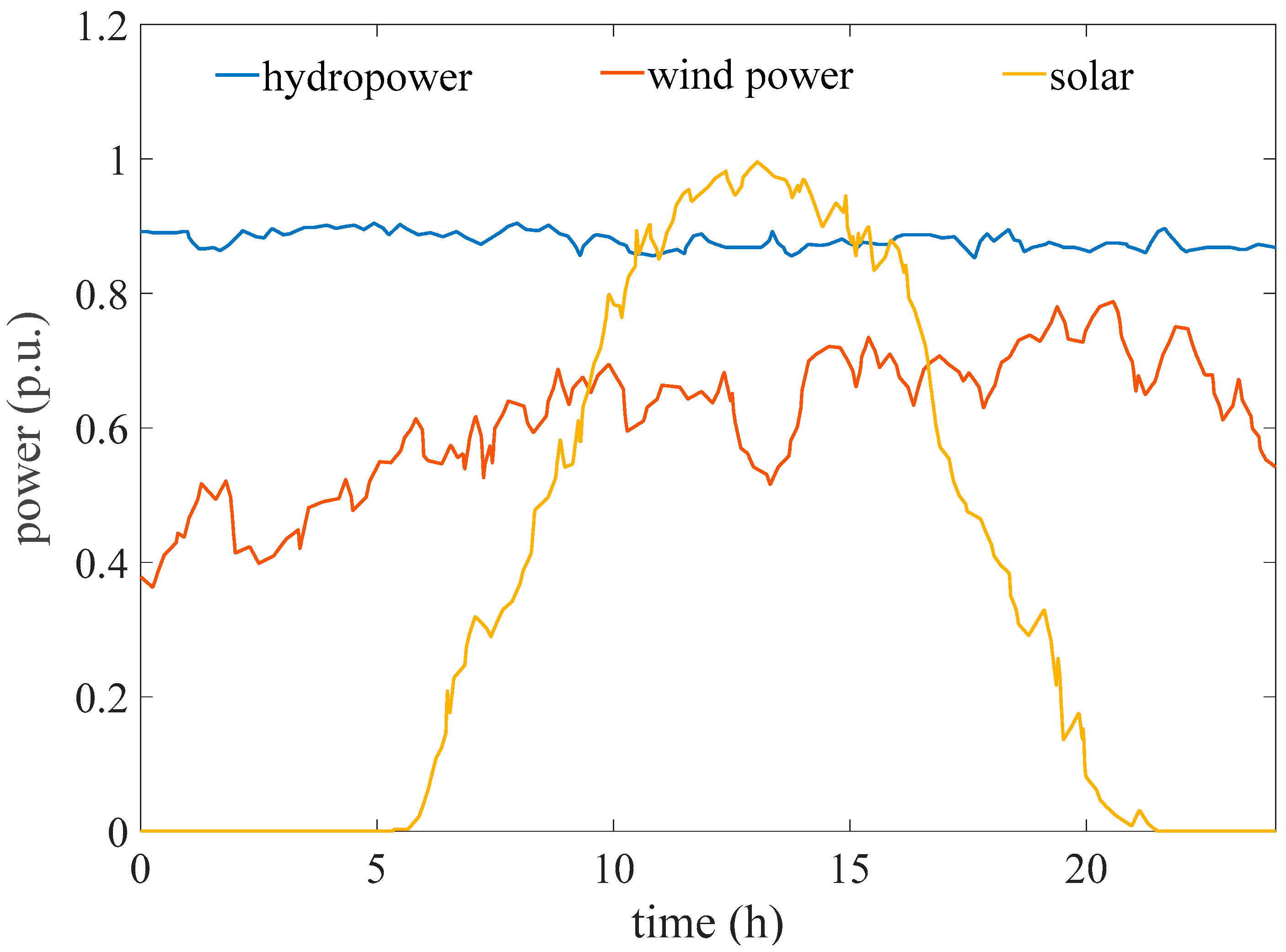
To investigate the operational performance of a wind–solar–hydro hybrid power system, the average fluctuation magnitude, Richards–Baker flashiness, the average climbing rate and the change in the time-averaged value are proposed to evaluate the fluctuation from a single perspective and entropy weight theory is used to transform the four evaluation indicators into a comprehensive evaluation indicator. Meanwhile, the load tracking coefficient and coupling degree are established to describe the complementarity of the hybrid power system. Using the proposed indices, the operational properties of the single and hybrid systems considering four different time scales are quantitatively analyzed based on a case study. The main conclusions from this work can be drawn as follows:

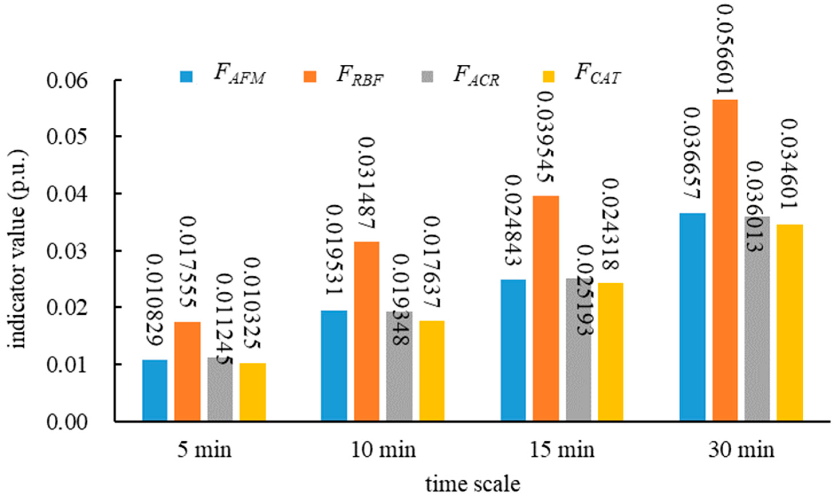
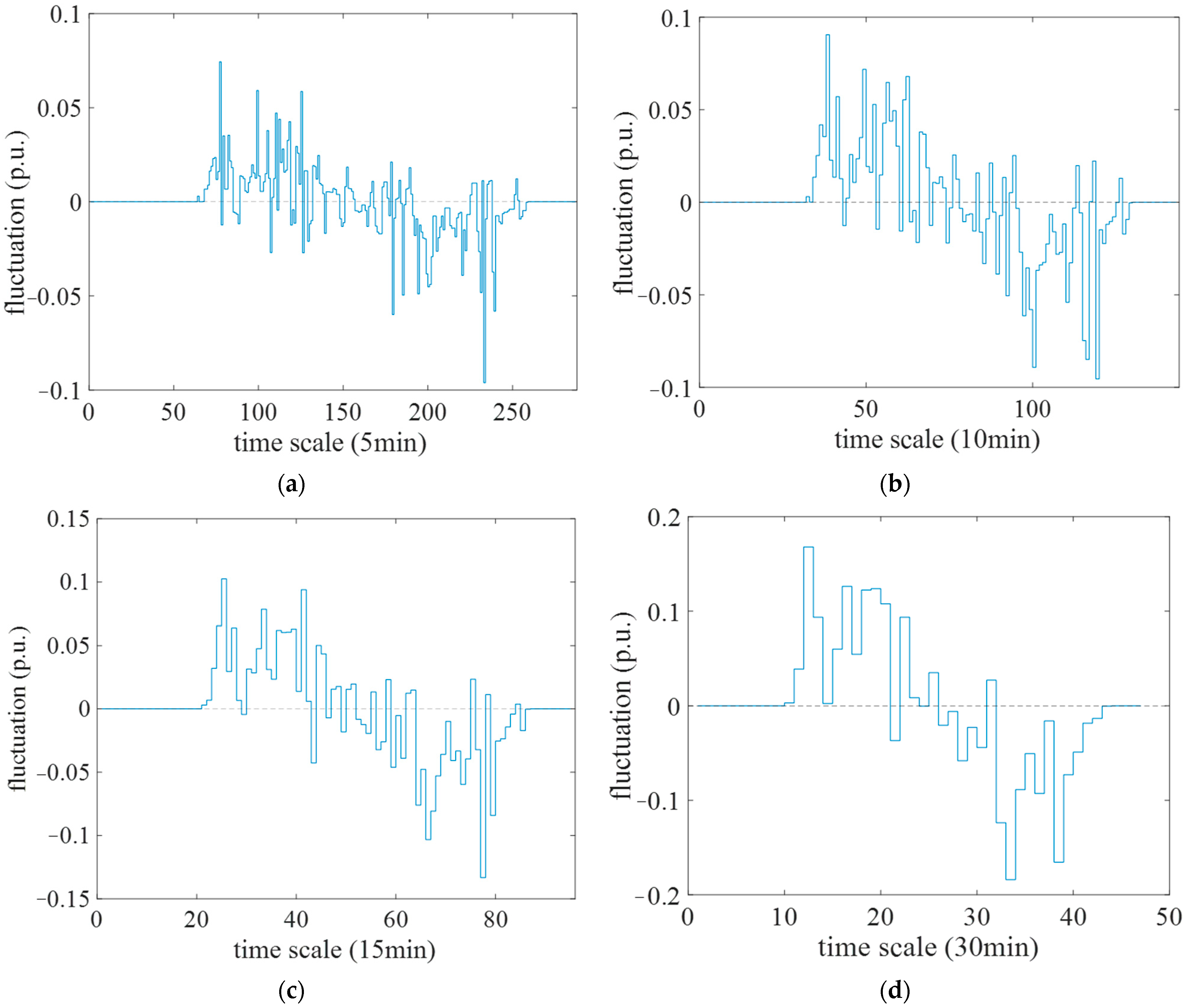
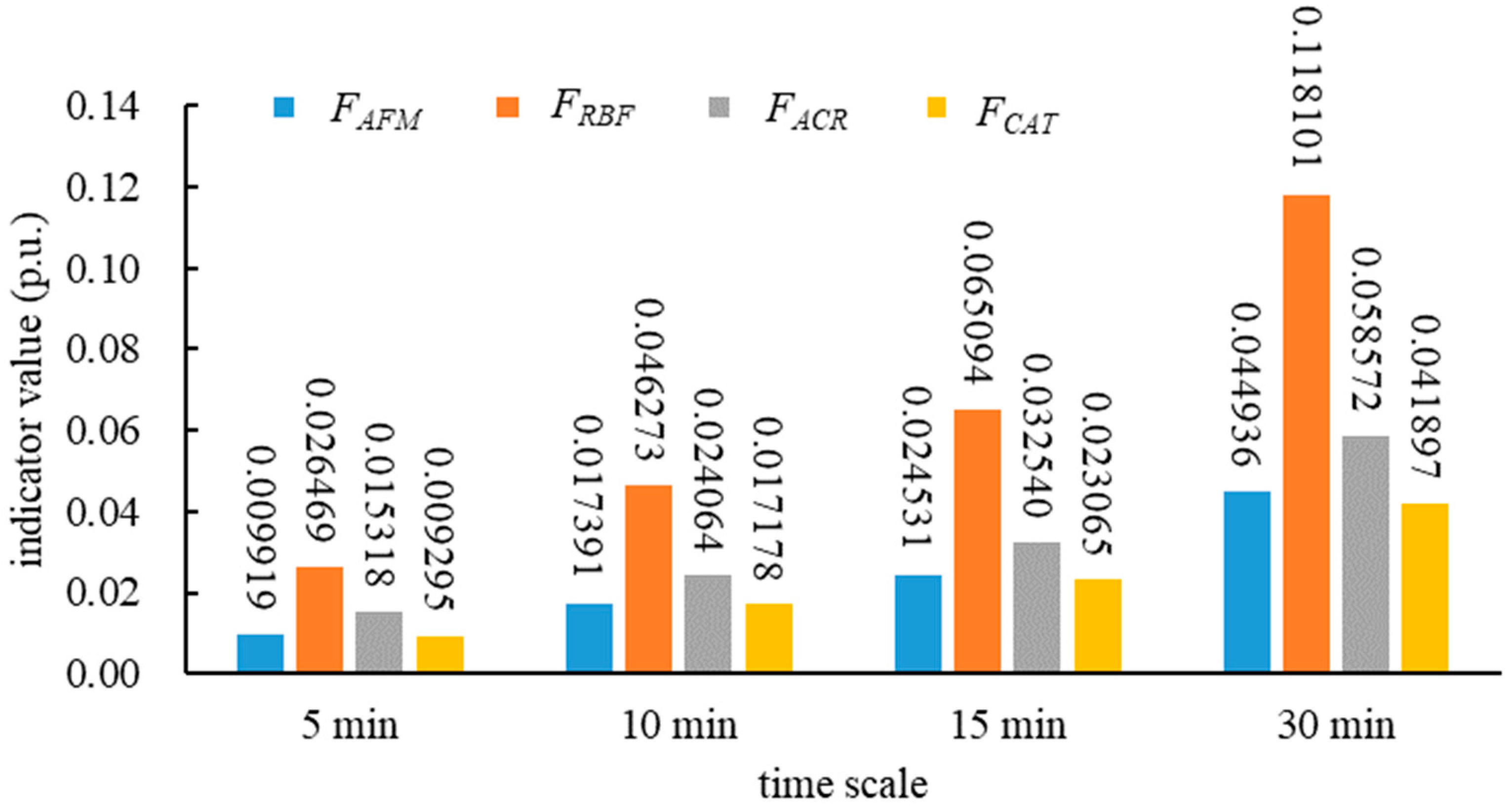
(1) Under a single-evaluation-indicator system, the maximum fluctuation magnitude of wind and solar power systems increases with the time scale increasing. The fluctuation of wind, solar, and hydropower increase with the time scale increasing at the 5 to 30 min time scale, i.e., the fluctuation becomes more severe with the increase in time scale. Meanwhile, the fluctuation of the hybrid system is less than that of an individual power system at the 5 min, 10 min, 15 min and 30 min time scales.

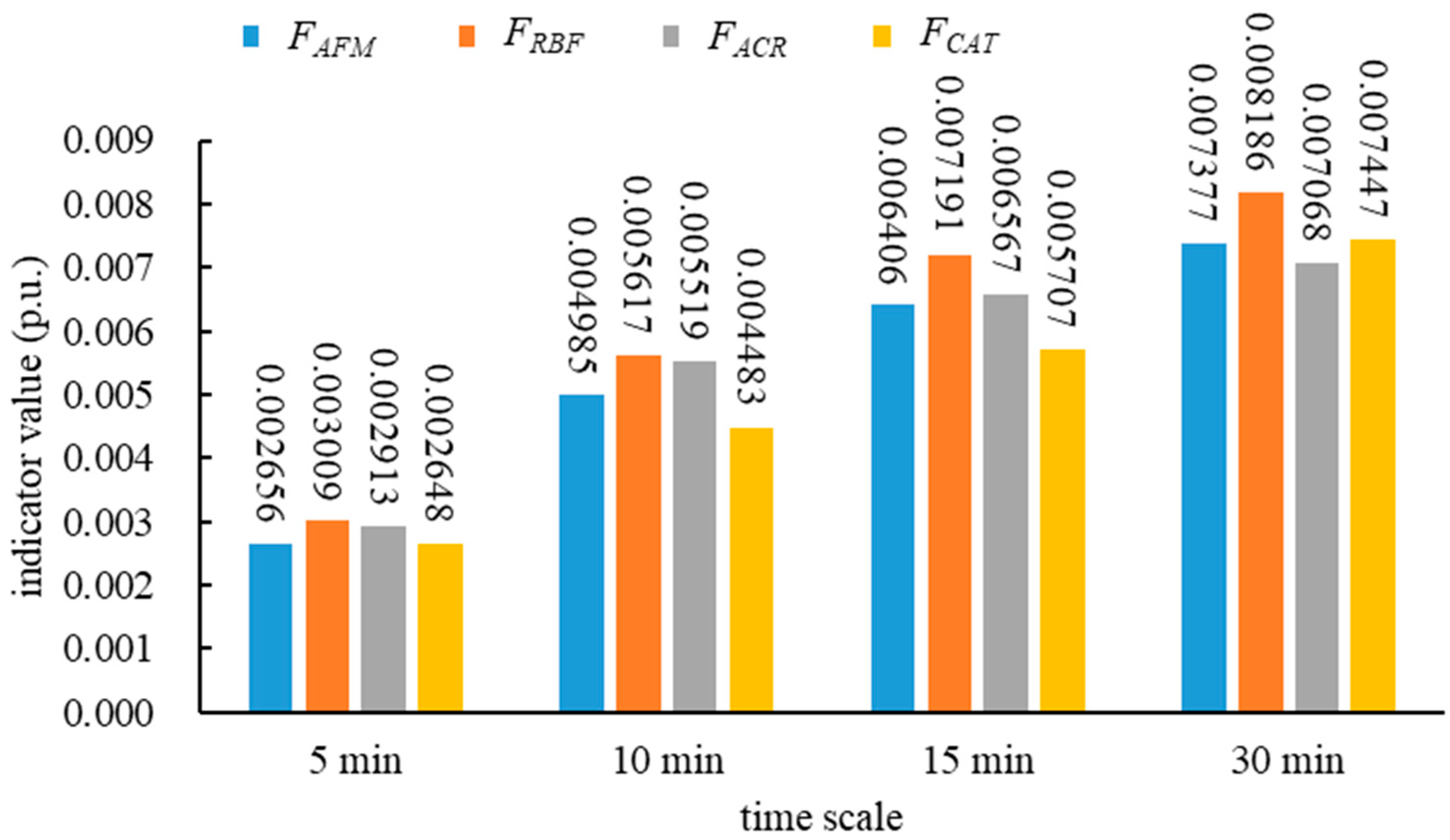
(2) Comprehensive assessment of volatility shows whether it is an individual power system or a combined power system—the fluctuation shows an upward trend with the increase in time scale. The comprehensive evaluation index of hydropower is the smallest, followed by that of wind–solar–hydro hybrid power systems, wind–solar hybrid power systems, wind power systems, and solar power systems. In other words, the fluctuation of the hybrid power system is weakened compared with an individual power system. The minimum comprehensive indicator of the hybrid power system is 0.008094 at the 5 min time scale, and the maximum is 0.028399 at the 30 min time scale. These phenomena mean that the complementarity among different power sources suppresses the fluctuation of wind and solar power.

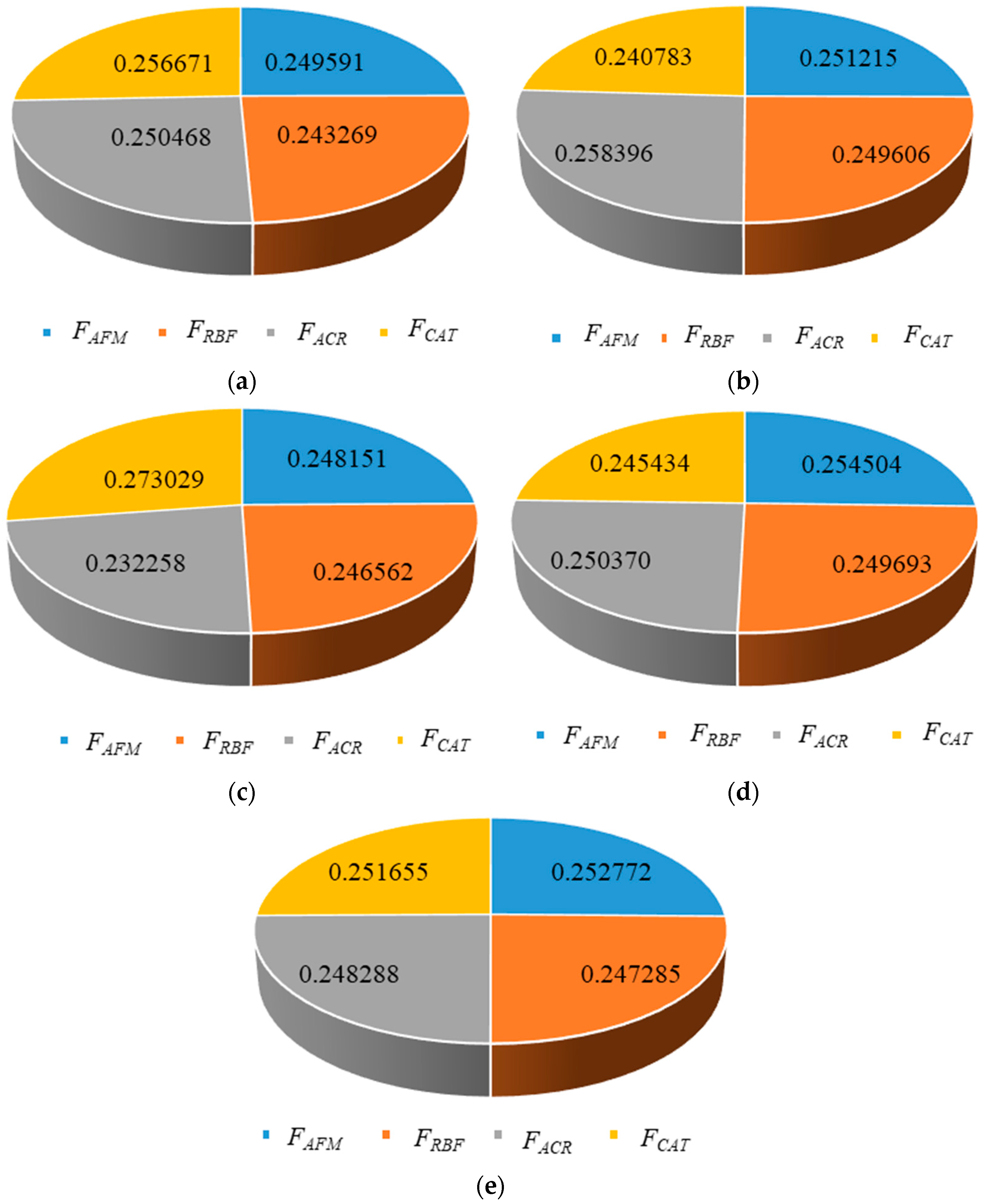
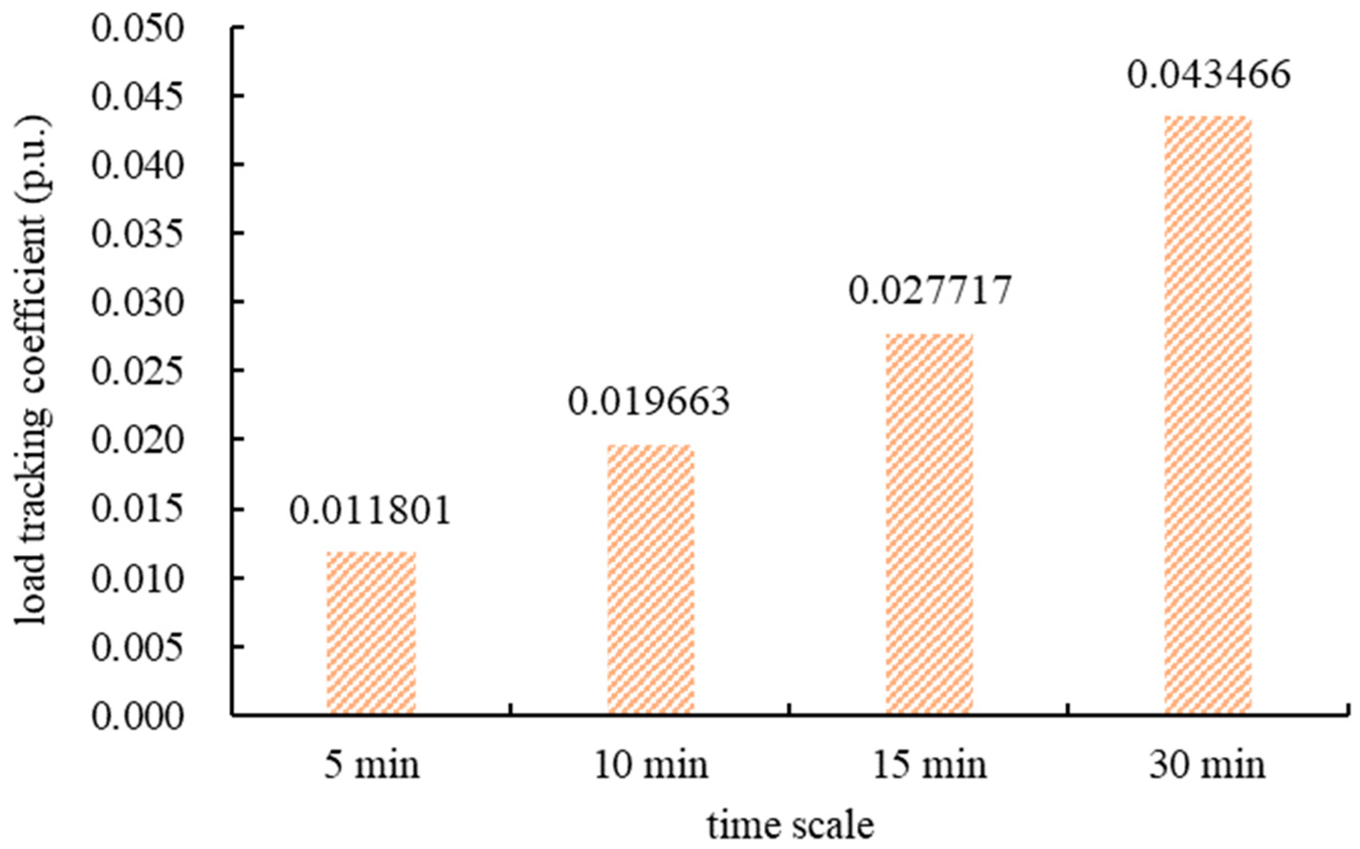
(3) Complementarity assessment is implemented based on the load tracking coefficient and coupling degree. The load tracking coefficient increases with the time scale increasing, meaning that the complementarity of a wind–solar–hydro hybrid power system on a smaller time scale is better than that on a larger time scale. The maximum and minimum load tracking coefficients are 0.082861 (30 min time scale) and 0.0309815 (5 min time scale), respectively. The degree of coordinated development among wind, solar, and hydropower is relatively high over a larger time scale. The contribution of hydropower is the highest and that of solar is the lowest at the time scale considered. The maximum and minimum coupling degree of the hybrid power system is 0.46235 and 0.457863, respectively, occurring at the 5 and 10 min time scales.

This paper takes time scale into account to investigate the fluctuation and complementary from single and comprehensive points of view, respectively. The proposed evaluation indicators are based on statistical theory, and the evaluation results are related to the size and distribution of the data volume. The distribution of power system output is influenced by the analysis period. Meanwhile, the assessment results do not involve a more detailed comparison among different installed capacity ratios of different energy sources owing to the limitation of data. The installed capacity ratio is a foreseeable key factor that affects the operational characteristics of the hybrid power system. Comparative results related to the analysis period and the installation ratio will be the topics of interest for future works.

References

1. IRENA. Renewables 2023 Global Status Report; The International Renewable Energy Agency: Abu Dhabi, United Arab Emirates, 2022. [Google Scholar]
2. IRENA. Renewable Energy Statistics 2022; The International Renewable Energy Agency: Abu Dhabi, United Arab Emirates, 2022. [Google Scholar]
3. National Energy Administration. Notice of the National Energy Administration on the Completion of the Responsibility Weights for Renewable Energy Electricity Consumption in 2021; National Energy Administration: Beijing, China, 2021. [Google Scholar]
4. IRENA. China’s Route to Carbon Neutrality: Perspectives and the Role of Renewables; The International Renewable Energy Agency: Abu Dhabi, United Arab Emirates, 2022. [Google Scholar]
5. IRENA. Renewable Energy Statistics 2023; The International Renewable Energy Agency: Abu Dhabi, United Arab Emirates, 2023. [Google Scholar]
6. Xu, B.B.; Zhang, J.J.; Egusquiza, M.; Zhang, J.Z.; Chen, D.Y.; Egusquiza, E. Exploring the regulation reliability of a pumped storage power plant in a wind-solar hybrid power generation system. Water 2021, 13, 2548. [Google Scholar] [CrossRef]
7. Zhang, J.J.; Li, H.H.; Chen, D.Y.; Xu, B.B.; Mahmud, A. Flexibility assessment of a hybrid power system: Hydroelectric units in balancing the injection of wind power. Renew. Energy 2021, 171, 1313–1326. [Google Scholar] [CrossRef]
8. Prebeg, P.; Gasparovic, G.; Krajacic, G.; Duic, N. Long-term energy planning of Croatian power system using multi-objective optimization with focus on renewable energy and integration of electric vehicles. Appl. Energy 2016, 184, 1493–1507. [Google Scholar] [CrossRef]
9. Hosseinalizadeh, R.; Shakouri, H.; Amalnick, M.S.; Taghipour, P. Economic sizing of a hybrid (PV–WT–FC) renewable energy system (HRES) for stand-alone usages by an optimization-simulation model: Case study of Iran. Renew. Sustain. Energy Rev. 2016, 54, 139–150. [Google Scholar] [CrossRef]
10. Zhang, C.; Zhou, J.Z.; Li, C.S.; Fu, W.L.; Peng, T. A compound structure of ELM based on feature selection and parameter optimization using hybrid backtracking search algorithm for wind speed forecasting. Energy Convers. Manag. 2017, 143, 360–376. [Google Scholar] [CrossRef]
11. Lian, J.; Zhang, Y.; Ma, C.; Yang, Y.; Chaima, E. A review on recent sizing methodologies of hybrid renewable energy systems. Energy Conv. Manag. 2019, 199, 112027. [Google Scholar] [CrossRef]
12. Zhang, Y.; Ma, C.; Lian, J.; Pang, X.; Qiao, Y.; Chaima, E. Optimal photovoltaic capacity of large-scale hydro-photovoltaic complementary systems considering electricity delivery demand and reservoir characteristics. Energy Conv. Manag. 2019, 195, 597–608. [Google Scholar] [CrossRef]
13. Xu, B.B.; Zhang, J.J.; Egusquiza, M.; Chen, D.Y.; Li, F.; Behrens, P.; Egusquiza, E. A review of dynamic models and stability analysis for a hydro-turbine governing system. Renew. Sustain. Energy Rev. 2021, 144, 110880. [Google Scholar] [CrossRef]
14. Rauf, H.; Gull, M.S.; Arshad, N. Complementing hydroelectric power with floating solar PV for daytime peak electricity demand. Renew. Energy 2020, 162, 1227–1242. [Google Scholar] [CrossRef]
15. Kougias, I.; Szabo, S.; Monforti-Ferrario, F.; Huld, T.; Bodis, K. A methodology for optimization of the complementarity between small-hydropower plants and solar pv systems. Renew. Energy 2016, 87, 1023–1030. [Google Scholar]
16. Tang, Y.J.; Fang, G.H.; Tan, Q.F.; Wen, X.; Lei, X.H.; Ding, Z.Y. Optimizing the sizes of wind and photovoltaic power plants integrated into a hydropower station based on power output complementarity. Energy Convers. Manag. 2020, 206, 112465. [Google Scholar] [CrossRef]
17. Fan, J.L.; Huang, X.; Shi, J.; Li, K.; Cai, J.W.; Zhang, X. Complementary potential of wind-solar-hydro power in Chinese provinces: Based on a high temporal resolution multi-objective optimization model. Renew. Sustain. Energy Rev. 2023, 184, 113566. [Google Scholar] [CrossRef]
18. Cheng, Q.; Liu, P.; Feng, M.Y.; Cheng, L.; Ming, B.; Luo, X.R.; Liu, W.B.; Xu, W.F.; Huang, K.D.; Xia, J. Complementary operation with wind and photovoltaic power induces the decrease in hydropower efficiency. Appl. Energy 2023, 339, 121006. [Google Scholar] [CrossRef]
19. Han, S.; Zhang, L.; Liu, Y.Q.; Zhang, H.; Yan, J.; Li, L.; Lei, X.H.; Wang, X. Quantitative evaluation method for the complementarity of wind-solar-hydro power and optimization of wind-solar ratio. Appl. Energy 2018, 236, 973–984. [Google Scholar] [CrossRef]
20. Li, H.H.; Mahmud, M.A.; Arzaghi, E.; Abbassi, R.; Chen, D.Y.; Xu, B.B. Assessments of economic benefits for hydro-wind power systems: Development of advanced model and quantitative method for reducing the power wastage. J. Clean. Prod. 2020, 277, 123823. [Google Scholar] [CrossRef]
21. Zhang, Y.S.; Lian, J.J.; Ma, C.; Yang, Y.; Pang, X.L.; Wang, L. Optimal sizing of the grid-connected hybrid system integrating hydropower, photovoltaic, and wind considering cascade reservoir connection and photovoltaic-wind complementarity. J. Clean. Prod. 2020, 274, 123100. [Google Scholar] [CrossRef]
22. Zhang, Y.S.; Ma, C.; Yang, Y.; Pang, X.L.; Lian, J.J.; Wang, X. Capacity configuration and economic evaluation of a power system integrating hydropower, solar, and wind. Energy 2022, 259, 125012. [Google Scholar] [CrossRef]
23. He, Y.Y.; Hong, X.Y.; Wang, C.; Qin, H. Optimal capacity configuration of the hydro-wind-photovoltaic complementary system considering cascade reservoir connection. Appl. Energy 2023, 352, 121927. [Google Scholar] [CrossRef]
24. Zhou, Y.Z.; Zhao, J.X.; Zhai, Q.Z. 100% renewable energy: A multi-stage robust scheduling approach for cascade hydropower system with wind and photovoltaic power. Appl. Energy 2021, 301, 117441. [Google Scholar] [CrossRef]
25. Zhang, Z.; Wu, X.Y.; Liao, S.L.; Cheng, C.T. An ultra-short-term scheduling model for cascade hydropower regulated by multilevel dispatch centers suppressing wind power volatility. Int. J. Elect Power 2022, 134, 107467. [Google Scholar] [CrossRef]
26. Daneshvar, M.; Mohammadi-Ivatloo, B.; Zare, K.; Asadi, S. Two-stage stochastic programming model for optimal scheduling of the wind-thermal-hydropower-pumped storage system considering the flexibility assessment. Energy 2020, 193, 116657. [Google Scholar] [CrossRef]
27. Zhou, S.Y.; Han, Y.; Zalhaf, A.S.; Chen, S.H.; Zhou, T.; Yang, P.; Elboshy, B. A novel multi-objective scheduling model for grid-connected hydro-wind-PV-battery complementary system under extreme weather: A case study of Sichuan, China. Renew. Energy 2023, 212, 818–833. [Google Scholar] [CrossRef]
28. Ye, L.; Qu, X.X.; Yao, Y.X.; Zhang, J.T.; Wang, Y.F.; Huang, Y.H.; Wang, W.S. Analysis on intraday operation characteristics of hybrid wind-solar-hydro power generation system. Autom. Electr. Power Syst. 2018, 42, 158–164. [Google Scholar]
29. Kern, J.D.; Patino-Echeverri, D.; Characklis, G.W. The impacts of wind power integration on sub-daily variation in river flows downstream of hydroelectric dams. Environ. Sci. Technol. 2014, 48, 9844–9851. [Google Scholar] [CrossRef] [PubMed]
30. Baker, D.B.; Richards, R.P.; Loftus, T.T.; Kramer, J.W. A new flashiness index: Characteristics and applications to midwestern rivers and streams. J. Am. Water Resour. Assoc. 2004, 40, 503–522. [Google Scholar] [CrossRef]
31. Zhang, L.N. The Temporal-Spatial Fluctuation Characteristics of Wind Speed and Application in Multi-Energy Complementarity; North China Electric Power University: Beijing, China, 2019. [Google Scholar]
32. Sevlian, R.; Rajagopal, R. Detection and statistics of wind power ramps. IEEE Trans. Power Syst. 2013, 28, 3610–3620. [Google Scholar] [CrossRef]
33. Ikegami, T.; Urabe, C.T.; Saitou, T.; Ogimoto, K. Numerical definitions of wind power output fluctuations for power system operations. Renew. Energy 2018, 115, 6–15. [Google Scholar] [CrossRef]
34. Guo, H.Y.; Liu, J.S.; Cheng, H.Z.; Zhang, S.X.; Wang, L.H. Comprehensive evaluation of grid-connected distributed generation based on Fuzzy mathematics and combined weighting method. Mod. Electr. Power 2017, 34, 14–19. [Google Scholar]
35. Yao, Y.X.; Ye, L.; Qu, X.X.; Wang, W.S.; Fan, Y. Power cloud coupled model for wind-photovoltaic-hydro hybrid power generation system. Power Syst. Technol. 2021, 45, 1750–1756. [Google Scholar]
Figure 1. Basic information and data of the wind–solar–hydro hybrid power system in 24 h.
Water 15 04051 g001
Figure 2. Fluctuation range of wind power under different time scales. (a) Fluctuation range of wind power under 5 min time scale. (b) Fluctuation range of wind power under 10 min time scale. (c) Fluctuation range of wind power under 15 min time scale. (d) Fluctuation range of wind power under 30 min time scale.
Water 15 04051 g002
Figure 3. Fluctuation assessment of wind power under different time scales.
Water 15 04051 g003
Figure 4. Fluctuation range of solar power under different time scales. (a) Fluctuation range of solar power under 5 min time scale. (b) Fluctuation range of solar power under 10 min time scale. (c) Fluctuation range of solar power under 15 min time scale. (d) Fluctuation range of solar power under 30 min time scale.
Water 15 04051 g004
Figure 5. Fluctuation assessment of solar power under different time scales.
Water 15 04051 g005
Figure 6. Fluctuation range of hydropower under different time scales. (a) Fluctuation range of hydropower under 5 min time scale. (b) Fluctuation range of hydropower under 10 min time scale. (c) Fluctuation range of hydropower under 15 min time scale. (d) Fluctuation range of hydropower under 30 min time scale.
Water 15 04051 g006
Figure 7. Fluctuation assessment of hydropower under different time scales.
Water 15 04051 g007
Figure 8. Weight distribution of evaluation indicators under different output types. (a) Weight distribution of evaluation indicators for wind power systems. (b) Weight distribution of evaluation indicators for the solar power system. (c) Weight distribution of evaluation indicators for the hydropower system. (d) Weight distribution of evaluation indicators for wind–solar hybrid power sysI. (e) Weight distribution of evaluation indicators for the wind–solar–hydro hybrid power system.
Water 15 04051 g008
Figure 9. Load tracking coefficients at different time scales.
Water 15 04051 g009