Article

Landscape Ecological Risk Evaluation Study under Multi-Scale Grids—A Case Study of Bailong River Basin in Gansu Province, China

1
College of Resources and Environment, Gansu Agricultural University, Lanzhou 730070, China
2
College of Architecture and Art, Hefei University of Technology, Hefei 230601, China
3
College of Management, Gansu Agricultural University, Lanzhou 730070, China
*
Author to whom correspondence should be addressed.
Water 2023, 15(21), 3777; https://doi.org/10.3390/w15213777
Submission received: 21 September 2023 / Revised: 12 October 2023 / Accepted: 24 October 2023 / Published: 28 October 2023

Abstract

:
To solve grid-scale problems and evaluation indicator selection in landscape ecological risk index (LERI) evaluation, this paper takes the Bailong River Basin in Gansu Province (BLRB) as an example. The LERI evaluation formulae and optimal grid scales were determined by screening landscape indices and area changes in the LERI at different grid scales. The evaluation indices were finally obtained according to the landscape characteristics and the correlation analysis of the landscape index value. Through the statistical analysis of the area of the LERI at the grid scale of 1–6 km, the optimal grid scale was determined to be 5 km. There was little change in land use patterns, with the most significant increases in artificial surfaces at 3.29% and 3.58%, respectively. Cultivated land was the only land use type to decrease by 184.3 km2. The LERI drops with the reduced cultivated land area; the landscape ecological medium risk area and cultivated land keep the same spatial distribution. Due to the limitation of the topography, cultivated land is generally distributed below 2500 m altitude, so 2500 m becomes the turning point in the spatial distribution of the LERI. The medium risk below 2500 m dominates the LERI type. Reduced cultivated land was the leading cause of reduced ecological risk according to an overlay analysis. The study of LERI evaluations provides a theoretical basis for sustainable and ecological environmental protection in the BLRB.

1. Introduction

Landscape ecology is a new branch of environmental science, geography, and ecology that can be used to study the relationship between ecological processes and regional ecosystems at different landscape scales and spatial patterns, and by policy organisations [1]. It reflects the influence of other landscape features on the changes in spatial patterns [2]. Climate change and human activities pose increased risks to ecosystems and sustainable development [3,4]. The ecological environment is a prerequisite for social and economic development and a necessary safeguard for human survival [5]. The LERI reveals unfavourable consequences arising from natural or human activity [6]. Meanwhile, the LERI reflects changes in ecosystem characteristics resulting from changes in landscape heterogeneity [7]. The LERI can indicate the extent to which ecosystem function and structure have been disturbed.
The LERI is evaluated in terms of regional landscapes, which is a creative idea for the study of spatial heterogeneity and landscape pattern–process mutual feedback, which are the concerns of landscape ecology [8]. Xie used spatial autocorrelation and semi-covariance methods to analyse spatial distribution and gradient differences in the LERI in Poyang Lake [9]. The LERI method used the CLUE-S model to study the land type changes’ future characteristics and explored the LERI response to land use changes [10]. Jin assessed the regional ecological risk from the spatial pattern perspective, based on the land use changes in Delingha City [11]. Most studies have evaluated landscape ecological risk from no view, and few have been innovative in their evaluation methods.
LERI assessment requires selecting reasonable evaluation grids to obtain optimal evaluation results. Landscape pattern characteristics are sensitive to the size of the grid on which they are sampled, so the results of a LERI assessment may also be sensitive to the grid size [12]. Subdivided evaluation grids are a common method in LERI assessment [13]. When using the grid as an evaluation unit, the scale of the grid is mainly dependent on the actual situation of the study area and the researcher’s experience. Later, to specify the evaluation grid on an optimal scale, Karimian used 2–5 times the average area of the patches in the study area as the evaluation grid [14]. In addition, Liu and Yang attempted to search for the optimal scale magnitude by fitting the semi-variance function results of landscape indices with different scales [15,16]. GS+ software was used to analyse the values of landscape indices at different grid scales, and the optimal scale was considered to be 2150 m by the block-to-base ratio analysis. Chen analysed the LERI at different grid scales by creating a square grid of 4–10 km and fitting a semi-variance function, concluding that the optimal grid scale was 7 km [17]. Based on this, Zuo [18] tested the results of the LERI under different magnitudes with a semi-variance function by taking into account 2–5 times the patch area in the traditional study, and the optimal grid scale was 4 km. When the evaluation grid is not determined accurately, the evaluation results may not reflect the spatial heterogeneity of the LERI in a realistic way, so it is necessary to resolve the optimal scale before the evaluation [19].
Strengthening the evaluation of LERI, preventing and resolving major ecological and environmental risks, and improving the early warning ability of LERI are priority tasks for the construction of ecological civilization [20]. In general, commonly used assessment methods for the LERI are the risk source and sink method and the landscape index method, which are fundamentally based on the probability multiplied by the loss to calculate the risk. The landscape source and sink method is represented by a complex function of the superposition of multi-factor LERI, and the function relationship is unclear, so it is difficult to distinguish the mutual influence of the issues between the different factors [21]. The landscape index method focuses on the degree of deviation of the landscape mosaic relative to the optimal pattern [13]. The current mainstream LERI evaluation method remains the landscape index method. To solve the problems of the confusing use of landscape indices and scale selection of evaluation grids in previous studies, we innovated the LERI evaluation formula by re-screening landscape indices and determining the optimal scale.
The BLRB has a unique geographical location, belonging to the transition area from the Tibetan Plateau to the Loess Plateau. The topography and geomorphology affect the whole basin, with severe landscape fragmentation and a fragile ecological environment. The ecosystem disturbance in the BLRB has recently increased yearly. The LERI is high in the BLRB, which is affected by natural disasters such as landslides and mudslides [22]. Therefore, the study of landscape ecological risk in the BLRB, on the one hand, reveals the mechanism of regional landscape pattern change and the regional characteristics of the LERI. Meanwhile, it can innovate the LERI evaluation method and solve some problems existing in previous studies.
In light of these considerations, this research commences its investigation by delving into landscape characteristics. It includes compiling, selecting, and examining landscape indices that meet the criteria for constructing the LERI evaluation formula. Following the analysis of alterations in the spatial extent of landscape ecological risk across different grid scales, the study attempts to ascertain the most optimal grid. The selection of the landscape index and the determination of the optimal scale will help to optimise the LERI evaluation formula further. The study of the LERI will provide substantial support for resolving land use conflicts and contribute to the future landscape management of the ecosystem in the BLRB.
This study analyses land use change and the LERI across the basin from the sustainability perspective of the entire basin. Specifically, the research objectives are three: (1) to solve the current problem of confusion in the use of evaluation indexes in the LERI and to determine the optimal landscape index in LERI evaluation; (2) to explore the optimal scale for grid division in LERI evaluation; and (3) to construct a LERI evaluation index and to analyse the temporal and spatial changes in the LERI pattern of the study area from 2000 to 2020, to identify the main landscape types that influence LERI changes and adopt the most effective and sustainable methods to protect the environment. This study’s results will help explore the mechanism of landscape pattern change and the characteristics of the LERI in the basin, providing a scientific basis for sustainable development and ecological governance in other basins.

2. Materials and Methods

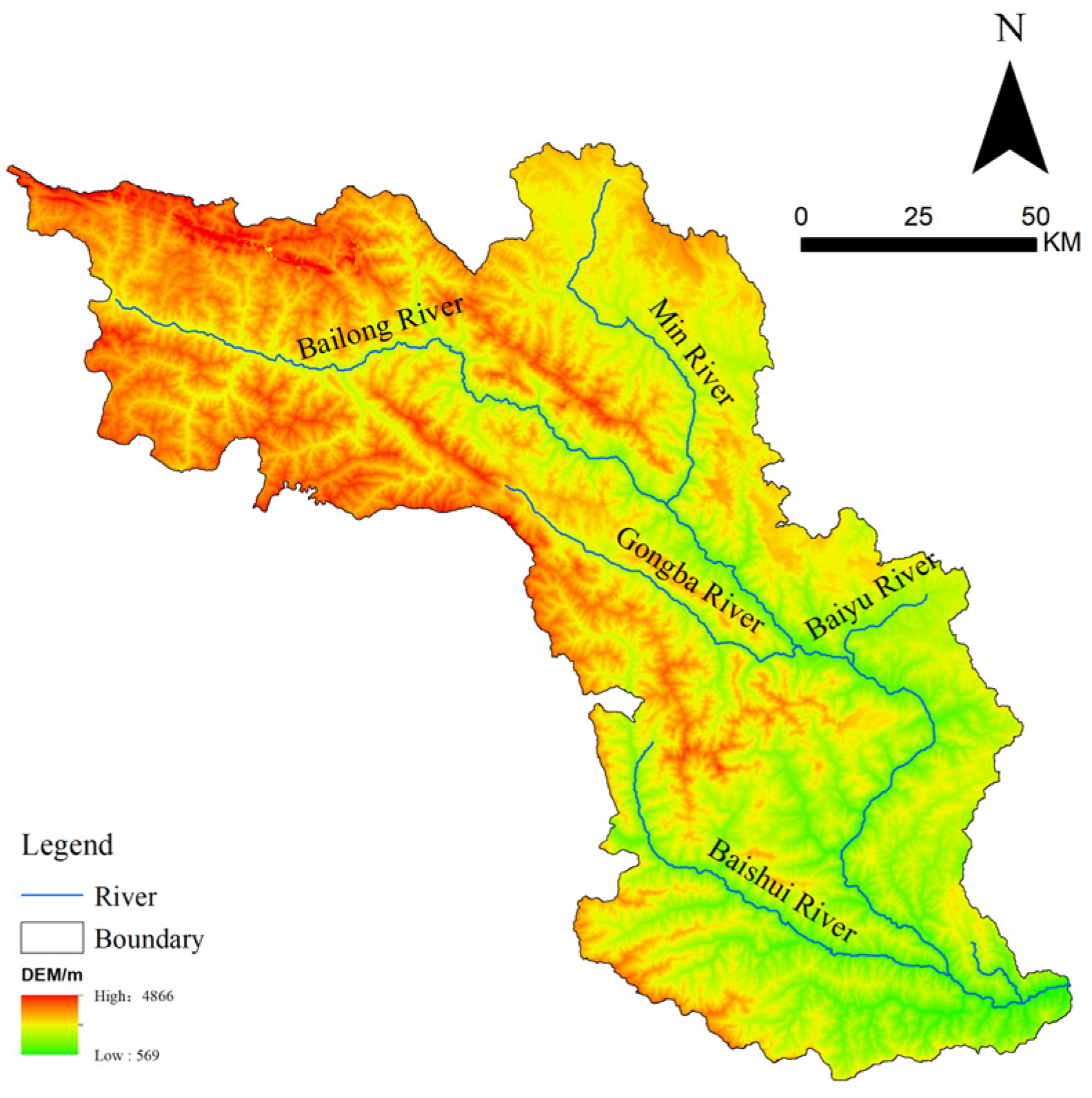
2.1. Overview of the Study Area

The BLRB (32°36′~34°24′ N, 102°48′~105°30′ E) is located in the southern part of Gansu Province (Figure 1). It is an essential ecological barrier area in the upper reaches of the Yangtze River. It mainly includes Wudu District, Diebu County, Zhouqu County, Tanchang County, and Wen County.
The terrain shows a high northwest and low southeast. The study area is a mountainous region with limited cultivated and artificial surfaces, and the population is mainly concentrated within the Bailong River Valley. The basin belongs to the transition area from a subtropical to a warm temperate area, with high temperatures and rain in summer and warm with little rain in winter, with an average annual precipitation of 400~850 mm. The rainy season is mainly concentrated between May and October, and the average yearly temperature is about 6~14.9 °C. The land use types in the study area are dominated by forest and grassland. At the same time, the BLRB is also the main production area of Chinese herbal medicine and olive oil and enjoys the reputation as “the hometown of thousand-year-old medicine” and “the city of olives”. In recent years, due to population relocation and urban development, the ecology has changed significantly, and how to evaluate the LERI through the optimal scale has become one of the research hotspots at the intersection of geography and landscape ecology. The flow of the study is shown in Figure 2.

2.2. Data Sources and Pre-Processing

Land use data for 2000, 2010, and 2020 were obtained from the website of the Resource and Environmental Science and Data Centre of the Chinese Academy of Sciences (https://www.resdc.cn, accessed on 3 April 2022). The spatial vector data and elevation data of the study area were obtained from the website of the National Basic Geographic Information Centre of China (https://ngcc.sbsm.gov.cn, accessed on 5 April 2022) and the Geospatial Data Cloud website (https://www.gscloud.cn, accessed on 5 April 2022). The land use data were classified into six major types: cultivated land, forest, grassland, water bodies, artificial surfaces, and bare land.

2.3. Attitudes towards Land Use Change

Land use dynamics refers to the rate of change of different types of land under the action of natural and human activities [23]. It is usually divided into the following two categories:
(1)
The degree of dynamic change in a single land use type. The rate of change in a particular land use type can be studied to quantitatively analyse the spatial pattern of land change, with the formula:
K = S b S a S a × 1 T × 100 %
where K is the dynamic degree of a land use type; Sa is the area of a land use type at the beginning of the study; Sb is the area of a land use type at the end of the study; and T is the study period.
(2)
The degree of dynamic change in integrated land use types. It can measure the difference in the overall speed of regional land use change with the formula:
S U = i = 1 n Δ L C i j 2 i = 1 n L C i × 1 T × 100 %
where LC is the comprehensive land use degree of a region during the study period; ΔLCi is the area of i land use type at the starting time; ∆LCi−j is the absolute value of the size of i land use type converted to the other land use types during the monitoring period; and T is the study period.

2.4. Landscape Index Selection

The landscape index is a simple quantitative index that can highly condense the information on landscape patterns and reflect its characteristics, such as structural composition and spatial structure [24]. Firstly, the existing landscape indices are counted according to patch level, type level, and landscape level, and there are 75 patch-level indices, 109 type-level indices, and 115 landscape-level indices. To use landscape indices to construct the LERI evaluation formula combines the ecological meaning of landscape indices, selects the corresponding landscape indices, and then the correlation analysis of the results of all the risky grids of the landscape indices finally determines the landscape indices that have strong representativeness and weak correlation to construct the LERI evaluation model. Since landscape indices reflect ecological conditions that vary at different landscape scales, determining the optimal study scale is the basis for LERI evaluation. According to the terrain characteristics such as connectivity, stability, fragmentation, dominance, separateness, aggregation, diversity and evenness, the landscape indices that reflect the landscape characteristics are selected as the optimal indices for calculating the LERI. A total of 15 landscape indices were chosen at the type level and 6 at the landscape level.
Considering the redundancy between indicators, it is necessary to carry out correlation tests for related indicators to ensure the independence of indicators. In the initial selection of evaluation indicators (Table 1), there is a duplication in indicator selection between the patch level and type level in the adjacent index, CONTIG, the fractal dimension index, FRAC, and the shape index, SHAPE, so when doing the correlation test, it is sufficient to consider only the indicators of the type level and the landscape level. The correlation between the indicators was calculated in Origin using the Spearman rank correlation method, which does not consider the assumption of normal distribution of the data. For land with a two-by-two correlation of landscape indices less than 0.8, the landscape index with a more negligible correlation with other landscape indices was selected for retention, considering the correlation of the index with other landscape indices [25]. All the indices were calculated based on the landscape analysis software, Fragstats 4.2. The ecological significance and calculation formula can be found in the operating instructions of the software or book, and the analysis results are shown in Table 2 and Table 3.
After the screening of landscape indices and correlation tests, six type-level indices and two landscape-level indices were obtained.

2.5. LERI Assessment Model Construction

As the indices were selected to facilitate the comparison and formula construction of landscape indices in different value ranges at a later stage [26], all the indices are standardised here with the following formulae:
X f = X i X min X max X min , X r = X max X i X max X min
where Xf is a positive indicator; Xr is a negative indicator; Xmax is the maximum value in the data; Xmin is the minimum value; and Xi is the data to be standardised.
Referring to previous studies, the independent weighting method [27] was chosen to assign values to obtain the LERI evaluation model with the following formula:
ERI = 0.16PD + 0.05LSI + 0.05CONTIG_MN + 0.32CONECT + 0.06LPI + 0.27SPLIT + 0.04SIDI + 0.05SIEI
According to the divided grid, each grid as an independent risk grid calculates each risk grid’s LERI index. The calculation results were assigned to each grid centroid for kriging interpolation to obtain the spatial distribution of LERI in the BLRB.

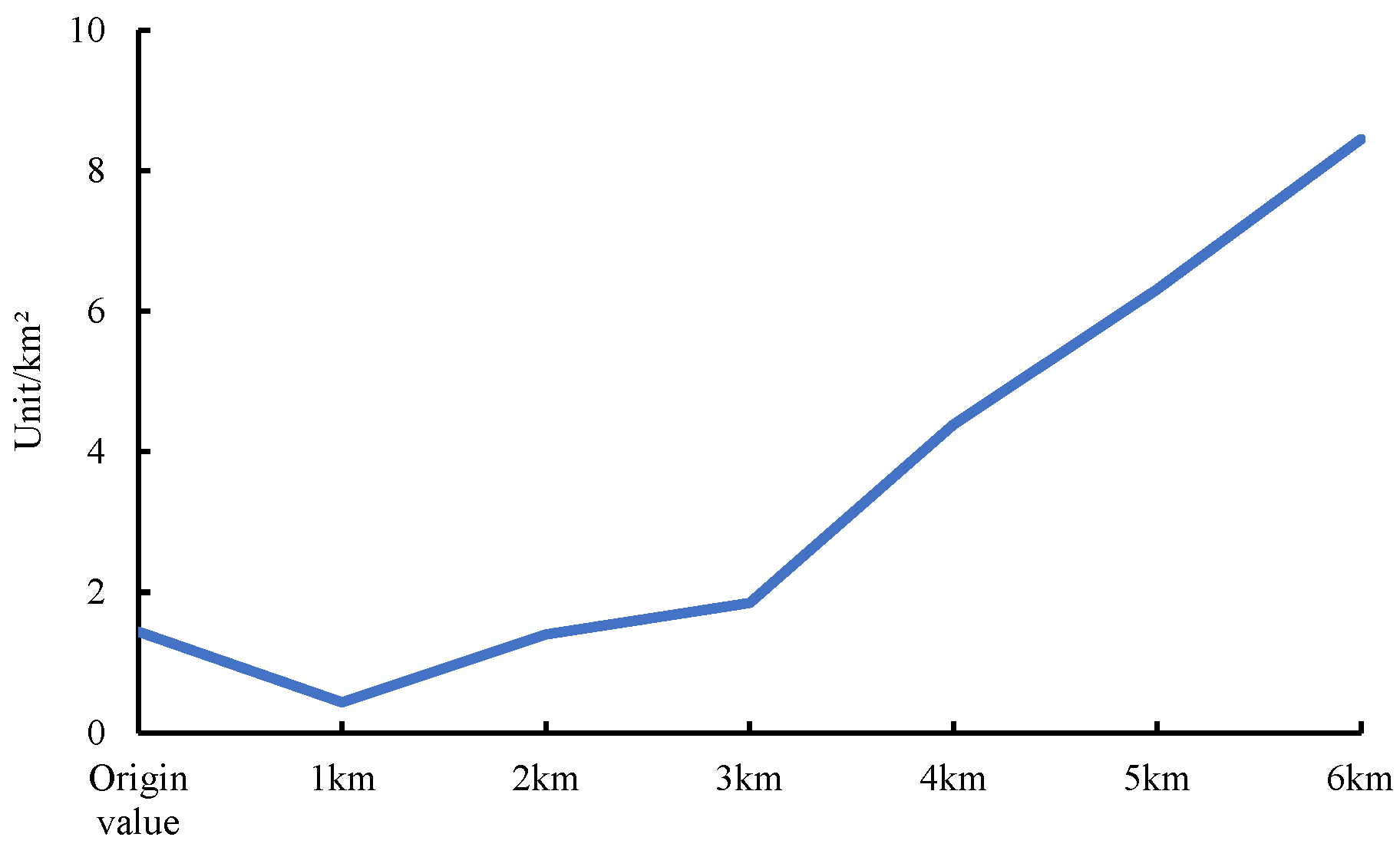
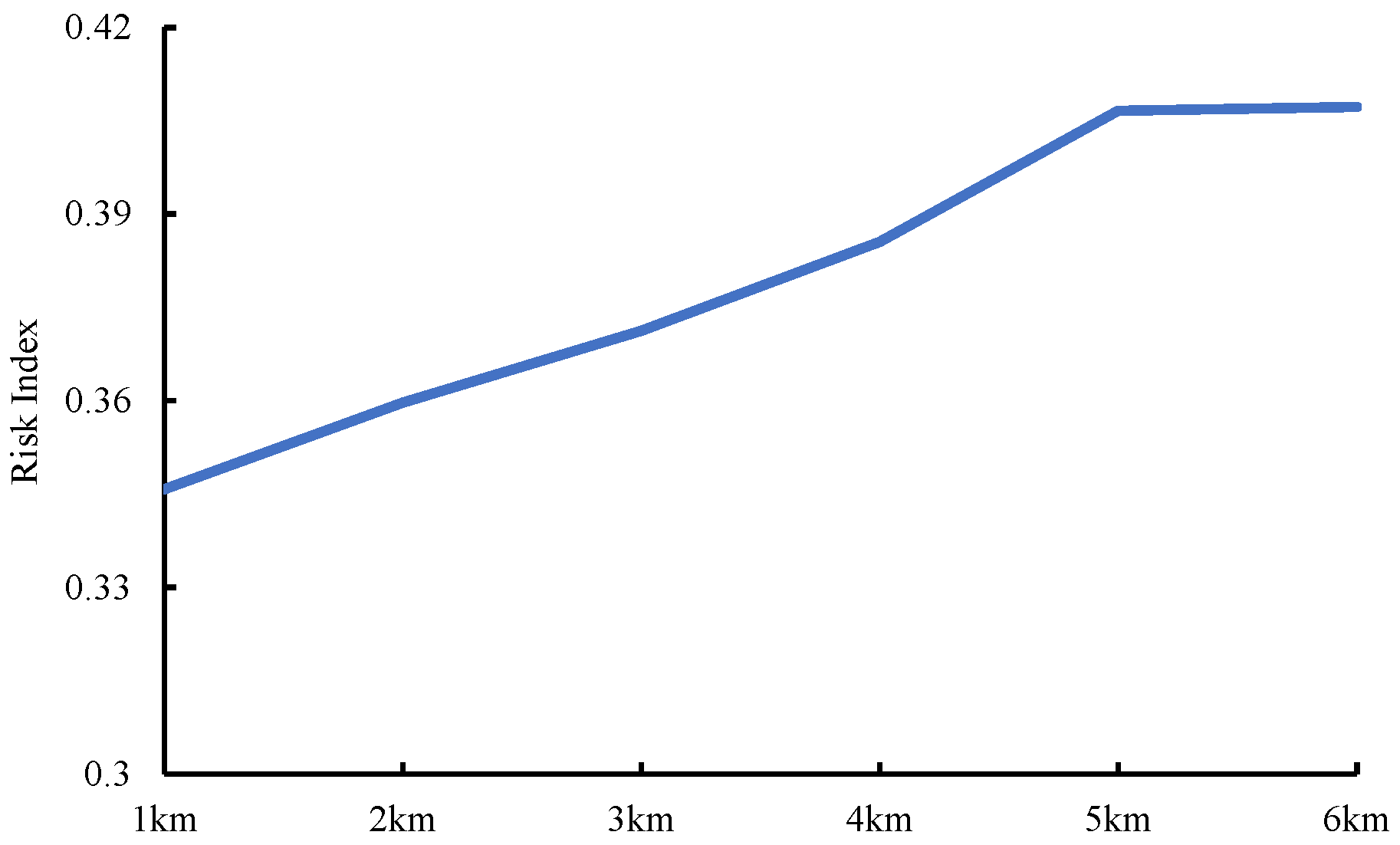
2.6. LERI Grid Determination

In previous studies, the designation of risk grids is generally 2–5 times the average patch area of the study area [28,29]. This method does not specify the size of the LERI evaluation grid, and the risk grid size selection is uncertain. To solve the problem of risk grid size selection, the study area was divided into six types of square grids of 1 km, 2 km, 3 km, 4 km, 5 km, and 6 km through the equal spacing method, and the LERI indices under different grid scales were calculated respectively.
The change in the average area of patches under different grid scales (Figure 3) and the middle area of patches shows a change process of decreasing and then increasing. The central location of patches of landscape components shows an increasing trend with the increase in the grid scale (Figure 4), among which the forest is most affected by the change in scale, and the construction land is least affected by the change in scale. Figure 5 shows the evolution of the average value of the LERI with the shift in the grid scale, and the LERI shows an increase and then tends to stabilise. This shows a trend of increasing and stabilising, and 5 km is the study scale at which the change in the LERI tends to stabilise. Since the LERI is an index determined by multiple indicators, it is challenging to decide on the optimal scale for LERI research by simply finding the optimal research scale for a certain number of landscape indices [30]. The optimal scale of the LERI is determined by studying the change in the LERI area under different scales. The changes in risk areas under different grid scales (Figure 6), which show the trend of lower risk areas decreasing and then increasing, and the size of medium risk areas increasing and then reducing by 5 km, belongs to the turning point of the area change of the LERI. At the same time, 5 km is the turning point of the LERI, which tends to be stabilised. Figure 7 shows the spatial distribution of risk areas at different scales. Therefore, it is determined that 5 km is the optimal scale for evaluating LERI.

2.7. Spatial Autocorrelation Analysis

GeoDa software was used to describe the spatial dependence of things to explore the spatial correlation of each risk grid in the study area of BLRB in different years through Moran’s I and local autocorrelation LISA significance maps [31].

3. Results

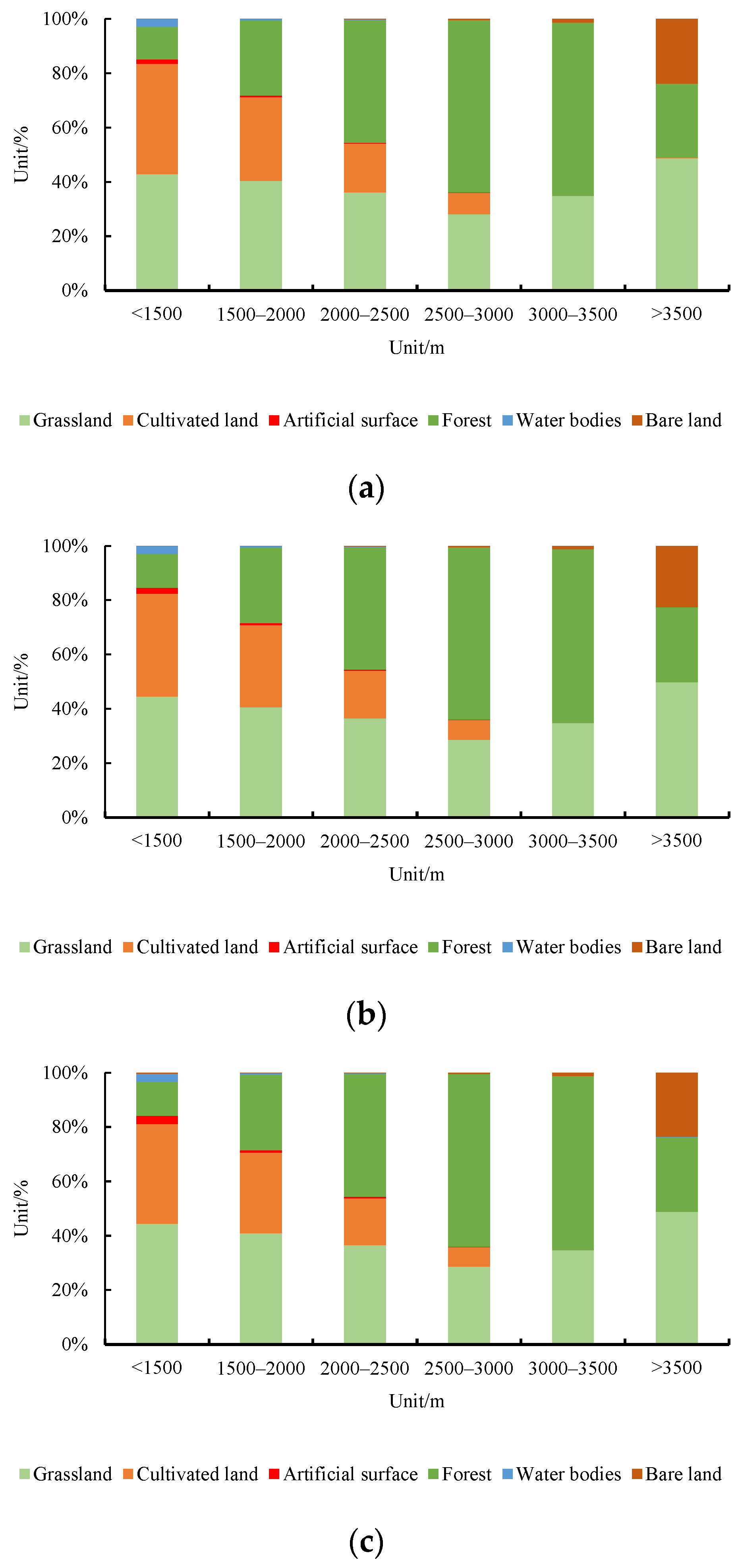
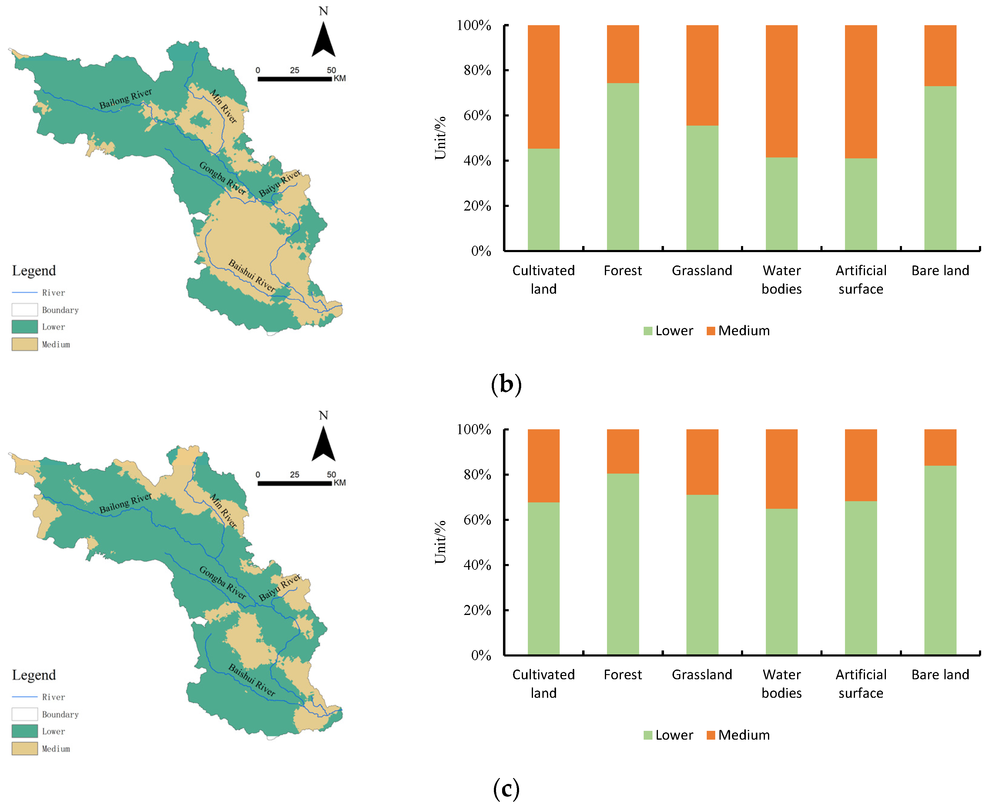
3.1. Analysis of Land Use Distribution and Its Dynamics

According to the degree of population concentration and topographic conditions of the study area, the BLRB is divided into six types according to altitude, namely, less than 1500 m, 1500–2000 m, 2000–2500 m, 2500–3000 m, 3000–3500 m, and more than 3500 m. Grassland and forest are the primary types, with grassland accounting for 37%. The proportion of grassland has been stable for three consecutive periods at 37%, and it is distributed in all the altitude ranges. Water bodies and artificial surfaces are mainly concentrated at less than 1500 m altitude. The artificial surfaces are distributed primarily in the altitude range below 2500 m and show a decreasing distribution trend in length. The proportion of forest increases with elevation in less than 3500 m spatial coverage. The space above 3000 m is mainly dominated by grassland and forest, and a small amount of bare land is distributed above 3500 m. The land use trend of the BLRB is as follows (Figure 8).
The land use dynamics of the BLRB are shown in Table 4 below, and the dynamics of artificial land are the highest in the study period, which are 3.29% and 3.58%, respectively, and belong to the type of land that increases continuously, with a total increase in artificial surfaces of 56.01 km2. Cultivated land has the lowest degree of change and belongs to the type of land that decreases continuously and dynamically, with a total decrease of 184.3 km2. Bare land shows a dynamic process of reducing and then increasing, but it is expanding, with a total increase of 10.91 km2. The rest of the land use types are dynamically growing. The integration of dynamic attitudes was 0.07% and 0.04% in the whole study area in 2000–2010 and 2010–2020, respectively. The total emotional attitude has not changed much and has slightly decreased with time. The main difference is shown in the area of cultivated land reducing, the size of grassland and artificial surface increasing, and the overall dynamic change in land use is more evident from 2000 to 2010.

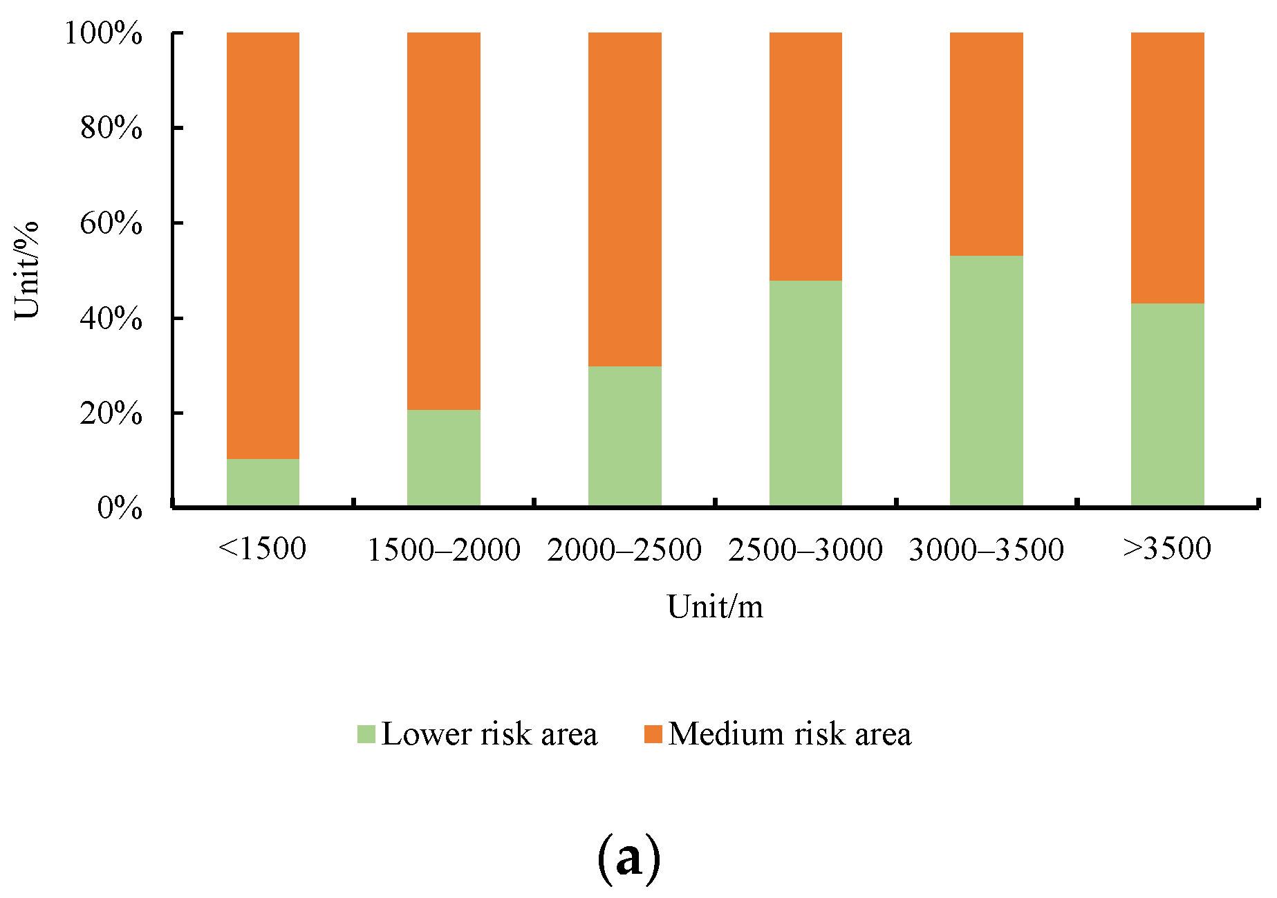
3.2. Analysis of Spatial and Temporal Changes in LERI

To more intuitively reflect the distribution of the LERI, spatial interpolation was carried out in ArcGIS software, based on the LERI values of each risk grid, and the study area was divided into low risk (0 ≤ LERI < 0.2), lower risk (0.2 ≤ LERI < 0.4), medium risk (0.4 ≤ LERI < 0.6), higher risk (0.6 ≤ LERI < 0.8), and high risk (0.8 ≤ LERI < 1). The values of the LERI in the three years were 0.24–0.58, 0.21–0.51, and 0.24–0.48, which showed that the distribution of the LERI was more concentrated and distributed in the medium- and lower-risk areas (Figure 9). During the study period, the maximum value of the LERI gradually decreased by year, and the LERI showed a contraction state. The LERI type is divided into medium and lower risk. The lower risk was 6374.4 km2, and the medium risk was 12026.22 km2. In 2010, the lower risk was 11496.03 km2, and the medium risk was 6904.59 km2. From 2000–2010, the medium risk decreased by 5121.63 km2, and the main areas of risk reduction are located in the northwestern part of the upper BLRB and the Minjiang River Basin. In 2020, the lower risk was 13792.1 km2, and the medium risk was 4608.52 km2. From 2010 to 2020, the medium risk decreased by 2296.07 km2, and the risk reduction was in the middle reaches of the BLRB and the two sides of the Baishui River. The LERI generally shows a decreasing trend from top to bottom along the BLRB on the time scale.
In Figure 10, it can be seen that the BLRB is the leading distribution area of medium risk below 2500 m altitude, with an area of 7759.64 km2 accounting for 42.17% of the basin. Above 2500 m above sea level is the main presence of the lower-risk areas, with an area of 4035.89 km2 accounting for 21.93% of the total area of the basin. Therefore, the LERI shows noticeable spatial distribution differences in the altitude gradient, and 2500 m is the turning point in the spatial distribution of the LERI. The spatial distribution of LERI has changed over time from top to bottom. From 2000 to 2010, the medium-risk areas above 2500 m altitude decreased by 2687.88 km2, accounting for 63% of the medium-risk areas in the region. The medium-risk areas below 2500 m altitude decreased by 2387.38 km2, accounting for 30.77% of the medium-risk area. Therefore, the medium-risk area distribution shows a noticeable gradient difference. By 2020, the medium risk is still distributed, accounting for 25% of the basin. The distribution in the LERI is not significantly affected by altitude, and the size of the lower-risk area is more dominant in high-altitude areas.

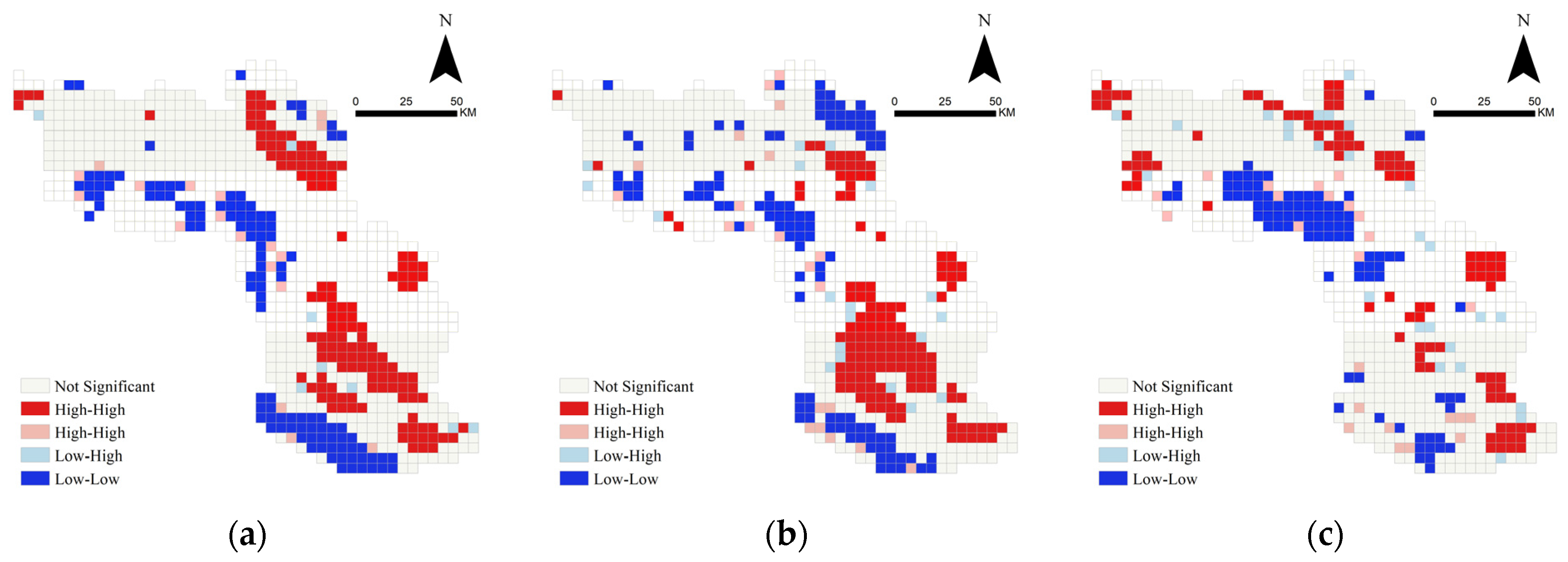
3.3. Spatial Autocorrelation Analysis

Moran’s I of the BLRB in 2000, 2010, and 2020 was 0.378, 0.329, and 0.262, respectively. The degree of LERI aggregation decreased over time. The distribution of local LISA clusters obtained by cluster analysis is shown in Figure 11. The types of aggregation are categorised as high-high aggregation(H-H), high-low aggregation (H-L), low-high aggregation (L-H), low-low aggregation (L-L), and no sign (NS). The LERI is dominated by H-H and L-L. The H-L is mainly distributed around the L-L, and the L-H exists more around the H-H. In 2000, there were 136 H-H grids distributed primarily in the northeastern and southeastern regions of the basin, and 110 L-L grids distributed mainly in the southwestern and western boundaries of the basin (Table 5). By 2010, the H-H and L-L in the northwestern and northeastern parts of the basin decreased, while the H-H in the northeast part of the Baishui River in the middle and lower reaches of the basin increased. By 2020, L-L in the northwestern part of the basin increased, and H-H decreased to 100, with presence only in the southeastern and northern regions. LERI clustering is dominated by H-H and L-L. The degree of spatial aggregation gradually decreases with time evolution, the number of H-H and L-L decreases, H-L and L-H gradually increases, and the number of grids of NS increases.

4. Discussion

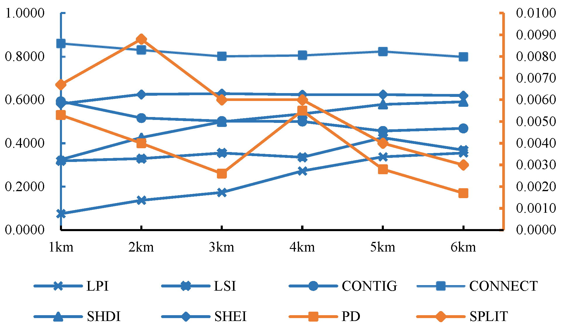
4.1. Landscape Indices and Scale Effects

In LERI evaluation, the previous researchers mainly selected several indices to characterise urban or basin LERI and its spatial characteristics based on a specific evaluation scale, and different studies obtained entirely different conclusions. The inconsistency between index selection and evaluation scale may be an essential reason for such results [32]. This study confirms that the response relationship between different landscape indices and the evaluation scale is also inconsistent, as shown in Figure 12.
Overall, the maximum patch index, LPI, and the landscape diversity index, SHDI, are more affected by the grid scale, which means that the LERI evaluation results are more likely to be affected by changes in the scale effects of the LPI and SHDI. Landscape indices such as maximum patch index, LPI, adjacent index, CONTIG, and connectivity index, CONNECT, were negatively correlated with the LERI, consistent with previous study findings. The four indices of fragmentation, separation, dominance, and fragility were selected for LERI evaluation in traditional studies, and the stability, connectivity, diversity, and evenness of the landscape were also taken into account, based on the previous research, so new indices were added in constructing the LERI evaluation formula. The evaluation formula of the vulnerability index and the evaluation formula of the LERI in many types of research have contradictions and similarities [33,34]. So, landscape vulnerability is not considered separately in constructing the new LERI evaluation formula. Through the calculation of the LERI under different scales, using the change curve of the mean value of the LERI and the change rule of varying LERI areas, the optimal grid scale for studying the LERI of BLRB was determined to solve the problem of the selection of the optimal scale grid in the calculation of the LERI.

4.2. Land Use and LERI Response Relationships

The distribution characteristics of land use reflect the space and extent of human activities. As an important ecological barrier area, BLRB is dominated by forests at a high altitude, and low-altitude areas are mainly located in the Bailong River Valley, which is mostly dominated by cultivated land and artificial surfaces, with drastic anthropogenic disturbances showing noticeable altitudinal differences. Thus, the LERI shows obvious gradient differences in the spatial gradients. During the study period, artificial interference land use significantly increased, closely related to urbanisation development and regional industrial characteristics. In the past two decades, areas unfavourable to agricultural production and human life have been restored under national policies, such as returning farmland to forests and ecological migration [35]. The corresponding cultivated land has been returned to forests and grasslands. The cultivated land has been continuously reduced in the study period, which is the main reason for the continuous reduction in the LERI. However, part of the cultivated land in the favourable natural environment has been encroached into by artificial surfaces. This is the main reason why some areas are medium-risk areas. The bare land is mainly concentrated in the space above 3500 m, and the new land expanded on the original basis during 2010–2020, increasing the area of bare land. The bare land is located at high altitudes and has poor natural conditions, with limited artificial intervention, which is difficult for regional LERI management.
In the study period, the overall change in land types is insignificant, but the mutual transformation between types is more prominent. The land use types and the overlap analysis of the LERI results are shown in Figure 10. It is found that there is a big gap between the distribution ratio of land types in different LERI types, the LERI of the same land use type changes more obviously in the study period, and the overall performance is that the lower-risk area increases, and the medium-risk area decreases. The medium-risk ratio of the basin, artificial surfaces, and cultivated land decreased from 94.86%, 93.41%, and 87.13% in 2000 to 35.05%, 31.63%, and 32.26% in 2020. This indicates that implementing land improvement and ecological management policies in the country recently has reduced the LERI and strengthened ecological protection. The study area’s LERI of forest land and bare land is relatively stable. The LERI of cultivated land, grassland, water bodies, and artificial surfaces is susceptible to changes due to human activities [36].
H-H and L-L decreased in the study area, and H-L and L-H increased around the L-L and H-H, respectively. It reflects that the type of LERI aggregation in some areas changed from the previous H-H to L-H, and the size of the high value of LERI started to decrease from outside to inside. In some areas, the type of LERI aggregation changed from the previous L-L to H-L, and the size of the low value of the LERI started to increase from inside to outside. In addition, the uncorrelated number of grids further increased, reflecting that the aggregation characteristics of the LERI decreased with time evolution. In general, with the transformation of the land use pattern, the spatial aggregation of the LERI gradually changed from the original H-H and L-L to H-L and L-H, which reflects the reduction in the LERI.

4.3. Applications and Shortcomings

Identifying the LERI based on different grid scales is conducive to systematically understanding the characteristics of varying landscape indices. This provides the basis for selecting evaluation scales for other landscape ecology studies. Although the evaluation of LERI is affected by different landscape indices and research scales [37], when the landscape’s chosen indices are constructed into the LERI evaluation formula, the average value of the LERI will eventually converge into a stable state with the changes in the research grids, which is of great significance in determining the optimal grid scale.
In this study, based on the previous research grid division [38,39], 1 km, 2 km, 3 km, 4 km, 5 km, and 6 km were used as the research scales to explore the scale effect of the LERI evaluation, which can provide a reference for the selection of landscape indices and the understanding of the LERI evaluation mechanism in the subsequent research. However, the effect of spatial resolution was not considered. At the same time, previous studies have confirmed that the difference in spatial resolution also affects the results of the landscape index and LERI, which will have an impact on the study’s results to a certain extent [40]. Meanwhile, to systematically reflect the scale characteristics of landscape indices and avoid omitting important indicators affecting the LERI, this study carried out the preliminary selection of ecological meanings and Spearman correlation analysis to identify the leading landscape indices affecting the LERI, which can ensure the scientific validity of the study. However, the core patch index, contrast-weighted edge density, edge contrast and similarity indices, and their practical significance for landscape spatial configuration are not easy to understand. There is no unified conclusion on the edge effect between different land use types, so this study does not use such indices for the time being; they need to be further explored in future research with practice. In addition, the BLRB is rich in land use types and has a characteristic spatial distribution. The study can evaluate the LERI scientifically by using the BLRB as a sample basin. However, because of the unique characteristics of the landscape pattern and territory of the BLRB, the study’s findings cannot directly explain the changes in LERI in other study areas with significantly different landscape characteristics. More samples of different types of basins need to be considered in future studies.

5. Conclusions

In sustainable development and ecological restoration, this study explores the influence mechanisms of land use and spatial characteristics of the LERI. Unlike the traditional landscape index method, it realises the LERI evaluation of the BLRB based on four aspects, including the ecological meaning of the landscape index, Spearman correlation analysis, grid-scale evolution, and spatial autocorrelation analysis. The innovation of this study is not only to introduce the grid-scale evolution into the LERI evaluation study but also to point out the new direction of the grid-scale selection study, to enrich the methods and criteria of grid selection, and to provide a universal theory contribution to LERI evaluation. In terms of a specific operation, the study first selected suitable indices to measure the LERI in the ecological meaning and correlation analysis of landscape indices. Secondly, the evolution of the LERI at different grid scales was analysed to determine the optimal scale for the study of LERI evaluation using the analysis of the mean value of the grid risk and the change in the landscape risk area. Finally, based on the results of the comments, recommendations are provided for the sustainable development of the basin. The study draws the following four conclusions: (1) By analysing the changes in the mean value of the LERI and the changes in the LERI areas at different grid scales, it is believed that 5 km is the optimal grid scale for studying the LERI. (2) The land use type of BLRB is dominated by forest and grassland. Cultivated land is mainly distributed below 2500 m. It is the only land use type that decreases continuously. The change in cultivated land is the main factor for the decrease in the LERI area. (3) The LERI shows a decreasing trend from 2000 to 2020. The proportion of the risk area and the degree of risk aggregation in the valley is significantly higher than that in other areas of the basin. Subject to the proportion of the area distribution of cultivated land on the altitude gradient, the altitude of 2500 m is the spatial turning point of the LERI. The lower-risk area is dominant in the space above 2500 m. The rate of reduction in the lower-risk area is more significant above 2500 m. (4) From 2000 to 2020, Moran’s I index declined slightly but was more critical than 0.2, and the LERI had a positive correlation and dispersed trend. The types of LERI aggregation are mainly dominated by H-H and L-L, with a relatively high significance level.
Based on the above conclusions, the following recommendations are made for the ecological protection and sustainable development of the basin: (1) Different measures should be taken for different risk types and spatial areas in ecological protection and restoration work. (2) Medium-risk areas are susceptible to external environmental disturbances, which can bring about a series of ecological restoration or reconstruction difficulties. In medium-risk areas, it is necessary to actively promote the restoration of damaged ecosystems and rationally plan land use. The mode and scale of development of cultivated land and artificial surfaces should be strictly controlled to avoid the continued expansion of medium-risk areas. (3) Sustainable economic, social, and ecological benefits develop through the establishment of a sound ecological compensation mechanism in lower-risk areas. In the future, quantitative research should be carried out on the factors of LERI changes while focusing on the deteriorating LERI and further deepening risk early warning research.
As valuable evaluation results, the findings of this study can be directly used to support decision-making processes. In a broader context, this work benefits those seeking similar assessments, mainly when conducting landscape assessments in ecological scale effects, as it reduces assessment uncertainty through a novel approach. However, there are some limitations to this study. Firstly, this study mainly considered the impact of different grid scales and ignored the result of grain size effects on LERI assessment. Secondly, the correspondence between other landscape indices and the LERI was not discussed. In addition, more detailed effects of land use change on the LERI in the western mountainous region are worth analysing. These will be explored in further research work, but they are unlikely to influence the main conclusions of this study.

Author Contributions

Conceptualization, Q.L. and X.L.; methodology, Q.L.; software, Q.L.; validation, X.L., Q.L. and L.Z.; formal analysis, B.M.; investigation, L.Z.; re-sources, Q.L.; data curation, Z.M.; writing—original draft preparation, Q.L.; writing—review and editing, Q.L.; visualization, L.L.; supervision, X.L.; project administration, X.L.; funding acquisition, X.L. All authors have read and agreed to the published version of the manuscript.

Funding

Research on Ecological Land Reclamation and Ecological Barrier Function in the Context of Multi-regulation: GAU-XZ-20160812.

Data Availability Statement

Not applicable.

Conflicts of Interest

The authors declare no conflict of interest.

References

  1. Xie, H.; Wen, J.; Chen, Q.; Wu, Q. Evaluating the landscape ecological risk based on GIS: A case study in the Poyang Lake region of China. Land Degrad. Dev. 2021, 32, 2762–2774. [Google Scholar] [CrossRef]
  2. Ran, P.; Hu, S.; Frazier, A. Exploring changes in landscape ecological risk in the Yangtze River Economic Belt from a spatiotemporal perspective. Ecol. Indic. 2022, 137, 108744. [Google Scholar] [CrossRef]
  3. Li, W.; Wang, Y.; Xie, S. Impacts of landscape multifunctionality change on landscape ecological risk in a megacity, China: A case study of Beijing. Ecol. Indic. 2020, 117, 106681. [Google Scholar] [CrossRef]
  4. Li, P.; Wu, J. Sustainable living with risks: Meeting the challenges. Hum. Ecol. Risk Assess. Int. J. 2019, 25, 1–10. [Google Scholar] [CrossRef]
  5. Xu, X.; Peng, Y.; Qin, W. Simulation, prediction and driving factor analysis of ecological risk in Savan District, Laos. Front. Environ. Sci. 2023, 10, 1058792. [Google Scholar]
  6. Li, B.; Yang, Y.; Jiao, L. Selecting ecologically appropriate scales to assess landscape ecological risk in megacity Beijing, China. Ecol. Indic. 2023, 154, 110780. [Google Scholar] [CrossRef]
  7. Hou, M.; Ge, J.; Gao, J. Ecological risk assessment and impact factor analysis of alpine wetland ecosystem based on LUCC and boosted regression tree on the Zoige Plateau, China. Remote Sensa 2020, 12, 368. [Google Scholar] [CrossRef]
  8. Li, Y.; Huang, S. Landscape Ecological Risk Responses to Land Use Change in the Luanhe River Basin, China. Sustainability 2015, 7, 16631–16652. [Google Scholar] [CrossRef]
  9. Xie, H.; Wang, P.; Huang, H. Ecological Risk Assessment of Land Use Change in the Poyang Lake Eco-economic Area, China. Int. J. Environ. Res. Public Health 2021, 10, 328–346. [Google Scholar] [CrossRef]
  10. Zhai, H.; Tang, X.; Wang, G.; Li, J.; Liu, K. Characteristic analyses, simulations and predictions of land use in poor mountainous cities: A case study in the central area of Chengde County, China. Environ. Earth Sci. 2018, 77, 585. [Google Scholar] [CrossRef]
  11. Jin, X.; Jin, Y.; Mao, X. Ecological risk assessment of cities on the Tibetan Plateau based on land use/land cover changes—Case study of Delingha City. Ecol. Indic. 2019, 101, 185–191. [Google Scholar] [CrossRef]
  12. Wang, B.; Ding, M.; Li, S.; Liu, L.; Ai, J. Assessment of landscape ecological risk for a cross-border basin: A case study of the Koshi River Basin, central Himalayas. Ecol. Indic. 2020, 117, 106621. [Google Scholar] [CrossRef]
  13. Cui, L.; Zhao, Y.; Liu, J.; Han, L.; Ao, Y.; Yin, S. Landscape ecological risk assessment in Qinling Mountain. Geol. J. 2018, 53, 342–351. [Google Scholar] [CrossRef]
  14. Karimian, H.; Zou, W.; Chen, Y.; Xia, J.; Wang, Z. Landscape ecological risk assessment and driving factor analysis in Dongjiang river watershed. Chemosphere 2022, 307, 135835. [Google Scholar] [CrossRef] [PubMed]
  15. Liu, Y.; Liu, Y.; Li, J.; Lu, W.; Wei, X.; Sun, C. Evolution of Landscape Ecological Risk at the Optimal Scale: A Case Study of the Open Coastal Wetlands in Jiangsu, China. Int. J. Environ. Res. Public Health 2018, 15, 1691. [Google Scholar] [CrossRef] [PubMed]
  16. Yang, K.; Xin, G.; Jiang, H.; Yang, C. Study on spatiotemporal changes of landscape risk based on the optimal spatial scale: A case study of Jiangjin district, Chongqing city. J. Ecol. Rural Environ. 2021, 37, 576–586. [Google Scholar]
  17. Chen, J.; Yang, Y.; Feng, Z.; Huang, R.; Zhou, G.; You, H. Ecological Risk Assessment and Prediction Based on Scale Optimization—A Case Study of Nanning, a Landscape Garden City in China. Remote Sensa 2023, 15, 1304. [Google Scholar] [CrossRef]
  18. Zuo, Q.; Zhou, Y.; Li, Q. Characteristics of spatial and temporal changes in landscape ecological risk in mountainous areas of Southwest Hubei based on optimal scales. Chin. J. Ecol. 2023, 42, 1186–1196. [Google Scholar]
  19. Ju, H.; Niu, C.; Zhang, S.; Jiang, W.; Zhang, Z.; Zhang, X. Spatiotemporal patterns and modifiable areal unit problems of the landscape ecological risk in coastal areas: A case study of the Shandong Peninsula, China. J. Clean. Prod. 2021, 310, 127522. [Google Scholar] [CrossRef]
  20. Asada, H.; Minagawa, T. Impact of Vegetation Differences on Shallow Landslides: A Case Study in Aso, Japan. Water 2023, 15, 3193. [Google Scholar] [CrossRef]
  21. Ai, J.; Yu, K.; Zeng, Z.; Yang, L.; Liu, Y.; Liu, J. Assessing the dynamic landscape ecological risk and its driving forces in an island city based on optimal spatial scales: Haitan Island, China. Ecol. Indic. 2022, 137, 108771. [Google Scholar] [CrossRef]
  22. Gong, J.; Liu, D.; Gao, B. Tradeoffs and synergies of ecosystem services in western mountainous China: A case study of the Bailongjiang basin in Gansu, China. J. Appl. Ecol. 2020, 31, 1278–1288. [Google Scholar]
  23. Li, D.; Zhou, J.; Zhan, D. Analysis of spatial and temporal changes and drivers of arable land in Heilongjiang province. Geogr. Sci. 2021, 41, 1266–1275. [Google Scholar]
  24. Shi, P.; Qin, Y.; Li, P. Development of a landscape index to link landscape patterns to runoff and sediment. J. Mt. Sci. 2022, 19, 2905–2919. [Google Scholar] [CrossRef]
  25. Xu, Z. Research on the Microclimate Impact Mechanism of Urban Mixed Commercial/Residential Neighbourhood Pattern; North University of Technology: Beijing, China, 2022. [Google Scholar]
  26. Yang, X.; Tan, M. Spatial difference of arable land function and its evolution in Beijing. Geogr. Res. 2014, 33, 1106–1118. [Google Scholar]
  27. Leng, Y.; Chen, Y.; Fu, Q. Assignment method for constructing boom index based on indicator independence. Stat. Decis. Mak. 2016, 19, 9–11. [Google Scholar]
  28. Moore, J.; Swihart, R. Modeling patch occupancy by forest rodents: Incorporating detect-ability and spatial autocorrelation with hierarchically structured data. J. Wildl. Manag. 2010, 69, 933–949. [Google Scholar] [CrossRef]
  29. Tian, P.; Li, J.; Shi, X. Spatial and temporal change of land use pattern and ecological risk assessment in Zhejiang Province. Resour. Environ. Yangtze River Basin 2018, 27, 59–68. [Google Scholar]
  30. Yan, J.; Li, G.; Qi, G. Landscape ecological risk assessment of farming-pastoral ecotone in China based on terrain gradients. Hum. Ecol. Risk Assess. Int. J. 2021, 27, 2124–2141. [Google Scholar] [CrossRef]
  31. Tong, Y. Spatial differentiation of Chinese traditional villages based on GIS. Hum. Geogr. 2014, 29, 44–51. [Google Scholar]
  32. Su, W.; Zhang, L.; Chang, Q. Coupled analysis of urban thermal environment and landscape features based on optimal granularity China. Environ. Sci. 2022, 42, 954–961. [Google Scholar]
  33. Zhang, J.; Run, C.; Dong, G. Spatial and temporal variability of landscape ecological vulnerability in the Li River. Res. Soil Water Conserv. 2022, 29, 283–292. [Google Scholar]
  34. Lu, Q.; Zhao, C.; Wang, J. Spatial and temporal evolution of landscape pattern vulnerability in Guizhou karst mountainous areas in the last 30 a Yangtze River Basin. Resour. Environ. 2022, 31, 634–646. [Google Scholar]
  35. Xie, Z.; Fan, S.; Du, S. Mechanism, risk, and solution of cultivated land reversion to mountains and abandonment in China. Front. Environ. Sci. 2023, 11, 1120734. [Google Scholar] [CrossRef]
  36. Zhao, Y.; Tao, Z.; Wang, M. Landscape Ecological Risk Assessment and Planning Enlightenment of Songhua River Basin Based on Multi-Source Heterogeneous Data Fusion. Water 2022, 14, 4060. [Google Scholar] [CrossRef]
  37. Liu, X. Progress of research on scale effects in landscape ecology in China. J. Gansu Agric. Univ. 2021, 56, 1–9. [Google Scholar]
  38. Zhang, H.; Xue, L.; Wei, G.; Dong, Z.; Meng, X. Assessing Vegetation Dynamics and Landscape Ecological Risk on the Mainstream of Tarim River, China. Water 2020, 12, 2156. [Google Scholar] [CrossRef]
  39. Zhang, J.; Hu, R.; Cheng, X. Assessing the landscape ecological risk of road construction: The case of the Phnom Penh-Sihanoukville Expressway in Cambodia. Ecol. Indic. 2023, 154, 110582. [Google Scholar] [CrossRef]
  40. Chen, X.; Yang, Z.; Wang, T.; Han, F. Landscape Ecological Risk and Ecological Security Pattern Construction in World Natural Heritage Sites: A Case Study of Bayinbuluke, Xinjiang, China. ISPRS Int. J. GeoInformation 2022, 11, 328. [Google Scholar] [CrossRef]
Figure 1. Topography of the BLRB.
Water 15 03777 g001
Figure 2. Flow chart of this study.
Water 15 03777 g002
Figure 3. Average patch size under different grid scales.
Water 15 03777 g003
Figure 4. Mean patch size of landscape types under different grid scales.
Water 15 03777 g004
Figure 5. Mean LERI under different grid scales.
Water 15 03777 g005
Figure 6. Area change in LERI under different grid scales.
Water 15 03777 g006
Figure 7. LERI distribution under different grid scales in 2000: (a) 1 km, (b) 2 km, (c) 3 km, (d) 4 km, (e) 5 km, and (f) 6 km.
Water 15 03777 g007
Figure 8. Spatial distribution of different land use types: (a) 2000, (b) 2010, and (c) 2020.
Water 15 03777 g008
Figure 9. Spatial distribution of other risk types: (a) 2000, (b) 2010, and (c) 2020.
Water 15 03777 g009aWater 15 03777 g009b
Figure 10. Spatial distribution of LERI: (a) 2000, (b) 2010, and (c) 2020.
Water 15 03777 g010aWater 15 03777 g010b
Figure 11. Landscape ecological risk aggregating analysis: (a) 2000, (b) 2010, and (c) 2020.
Water 15 03777 g011
Figure 12. Changes in mean landscape index under different scales.
Water 15 03777 g012
Table 1. Optimal landscape index.
Landscape-ScaleLandscape
Features
Primary IndexIndex of Passing
the Test
Patch metricsContiguityCONTIG
StabilityFRAC, SHAPE
Class metricsCrumblinessPDPD
DominanceLPILPI
StabilityLSI, SHAPE_MN, FRAC_MN, nLSILSI
ConnectivityCONTIG_MN, CONNECT, PLADJ, IJICONTIG_MN, CONNECT
SeparabilityDIVISION, SPLITSPLIT
AggregationCOHESION, AI, CLUMPY
Landscape metricsDiversitySHDI, SIDI, MSIDISHDI
EvennessSHEI, SIEI, MSIEISHEI
Table 2. Landscape indices correlation test.
PDLPILSICONTIG_MNCONNECTSPLITSHDISHEI
PD1
LPI−0.421
LSI0.5−0.731
CONTIG_MN0.2−0.50.781
CONNECT0.076−0.170.230.181
SPLIT0.11−0.250.480.610.161
SHDI0.37−0.650.730.640.160.171
SHEI0.19−0.390.17−0.0480.021−0.440.631
Table 3. Landscape indices and ecological implications.
Landscape-ScaleFeaturesIndex NameUnitsRangeEcological Implications
Class metricsCrumblinessPatch densitypcs/100 hm2>0The greater the PD, the greater the landscape fragmentation and the higher the LERI of the landscape.
DominanceLargest patch index%(0, 100]LPI represents the degree of dominance, with a larger LPI indicating that the dominant type in the landscape is more prominent and poses less LERI risk to the landscape.
StabilityShape index≥1LSI stands for stability, and a larger LSI indicates that the more complex the shape of the landscape component, the more unstable its structure, and the higher the LERI of the landscape.
Intra-patch connectivityAverage adjacency index[0, 1]CONTIG_MN stands for patch internal connectivity; the more significant the value, the better the connectivity within the patch and the lower the LERI of the formed landscape.
Inter-patch connectivityConnect Index%[0, 100]CONNECT represents the connectivity between patches. The larger the connectivity index, the better the connectivity between patches and the lower the LERI of the landscape.
SeparabilitySplit index≥1SPLIT represents the degree of separation of the same type of patches. The greater the splitting index, the greater the degree of separation between the same kind of patches, resulting in a higher LERI of the landscape.
Landscape metricsDiversityLandscape diversity index≥0The SHDI reflects the diversity of the landscape; the more significant the landscape diversity, the higher the LERI of the landscape.
EvennessLandscape evenness index[0, 1]The SHEI reflects the degree of homogeneity of the landscape; the more significant the landscape homogeneity, the higher the LERI of the landscape.
Table 4. Land use dynamics.
Type2000–20102010–2020
Area
Changes/km2
Homogeneous
Attitude/%
Area
Changes/km2
Homogeneous
Attitude/%
Cultivated land−116.03−0.38−68.27−0.23
Forest14.930.025.580.01
Grassland88.590.130.360
Water bodies1.690.206.540.76
Artificial surface22.903.2933.113.58
Bare land−11.77−0.3022.680.6
Integration of dynamic attitudes0.070.04
Table 5. Spatial autocorrelation aggregating statistics.
Years200020102020
Types
High-high136132100
Low-low11010589
High-low182124
Low-high81926
No sign579574612
Disclaimer/Publisher’s Note: The statements, opinions and data contained in all publications are solely those of the individual author(s) and contributor(s) and not of MDPI and/or the editor(s). MDPI and/or the editor(s) disclaim responsibility for any injury to people or property resulting from any ideas, methods, instructions or products referred to in the content.

