
Enhancing Runoff Simulation Using BTOP-LSTM Hybrid Model in the Shinano River Basin


Abstract
:1. Introduction
2. Materials
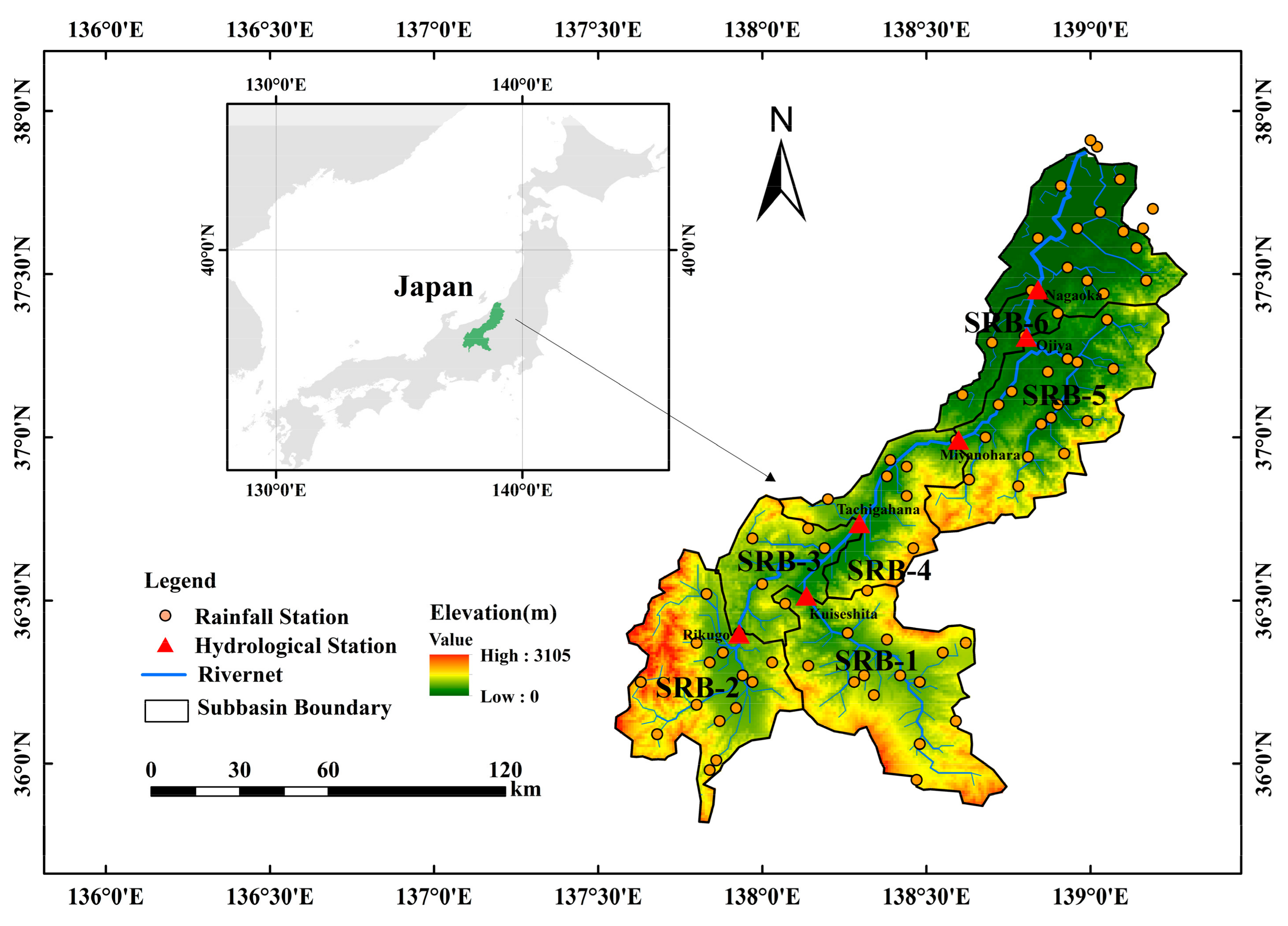
2.1. Study Area
2.2. Data
3. Methodology
3.1. Evaluation Criteria
3.2. Hydrological Model: The Block-Wise Use of TOPMODEL (BTOP Model)
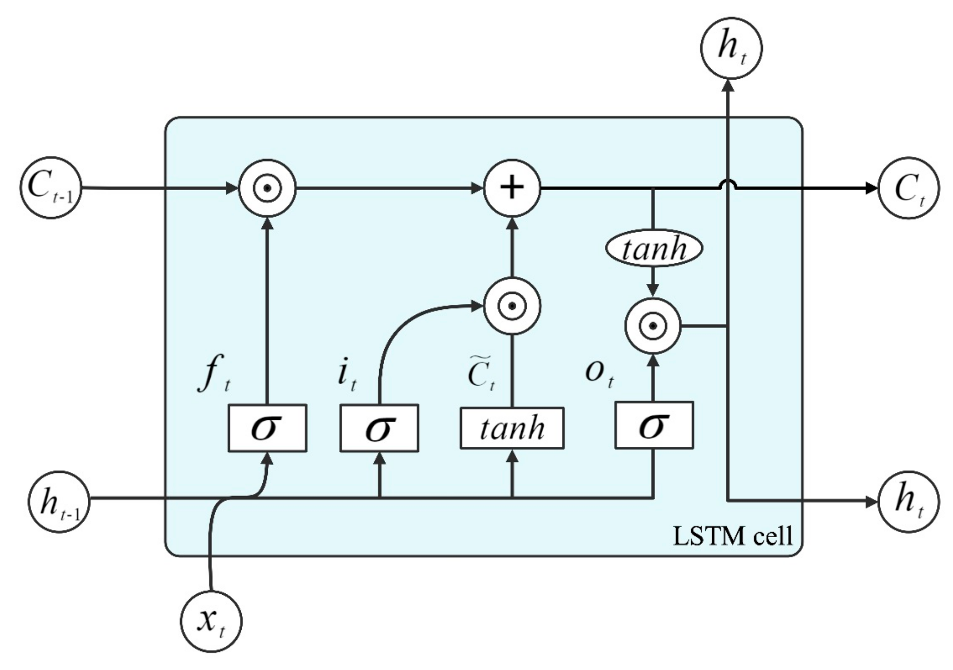
3.3. Long Short-Term Memory Network (LSTM)
3.4. Feature Dimensionality Reduction Method
3.4.1. Pearson Correlation Coefficient (PCC)
3.4.2. Principal Component Analysis (PCA)
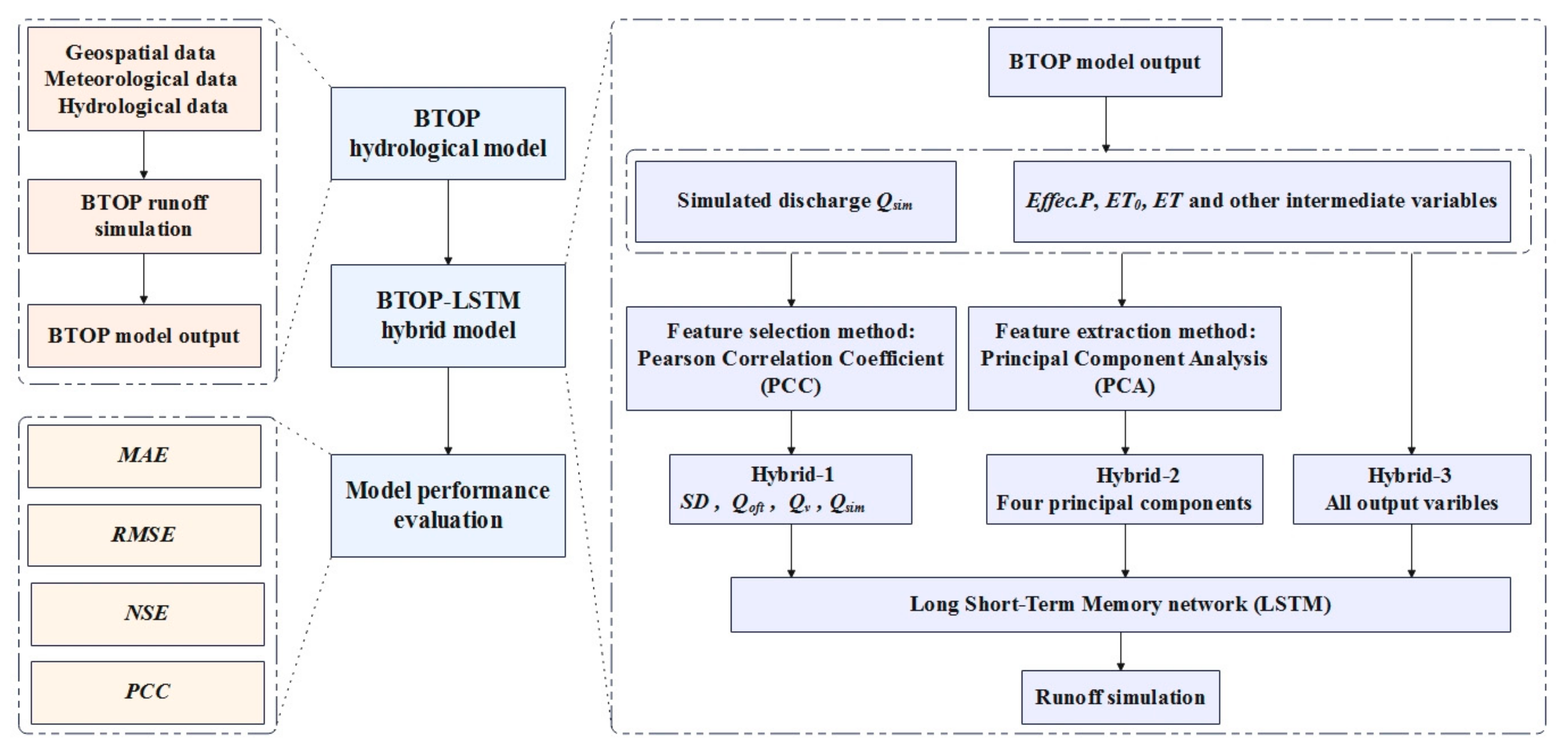
3.5. Model Design
3.5.1. Standalone LSTM Settings
3.5.2. Construction of Hybrid Models
- Hybrid-1: Pearson correlation analysis, a common feature selection method, was employed to screen the feature variables demonstrating high correlation with the observed discharge as additional input to the standalone LSTM.
- Hybrid-2: Employing principal component analysis as a feature dimensionality reduction method, converted eight input features into a few principal components and fed them as additional features into the standalone LSTM.
- Hybrid-3: All output variables from the BTOP model were directly fed into the standalone LSTM as additional features without any dimensionality reduction.
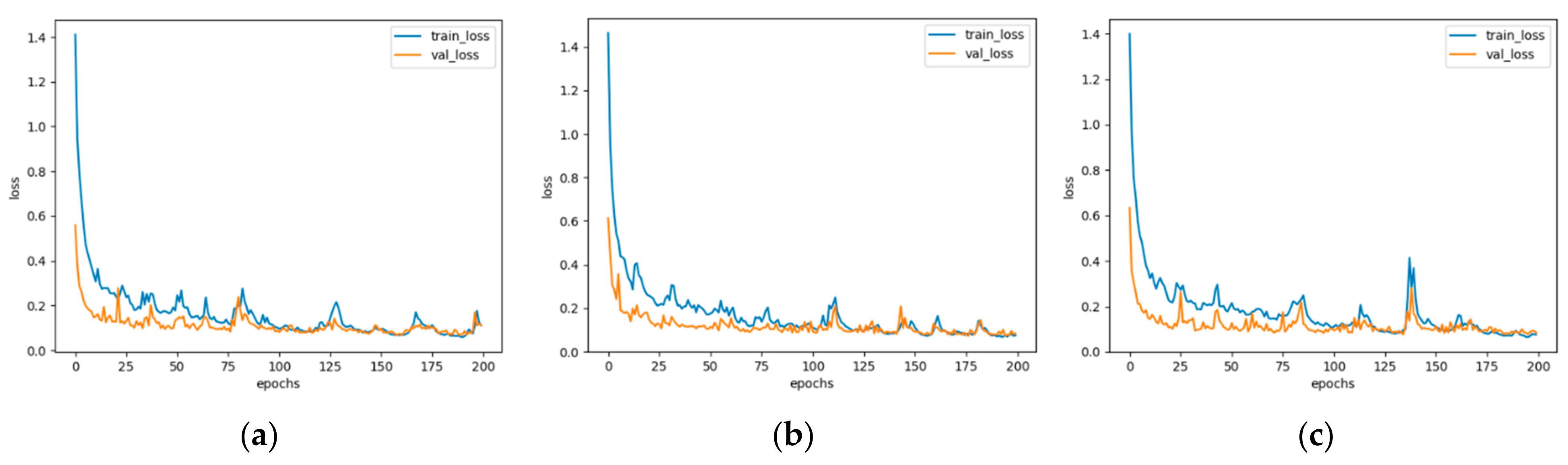
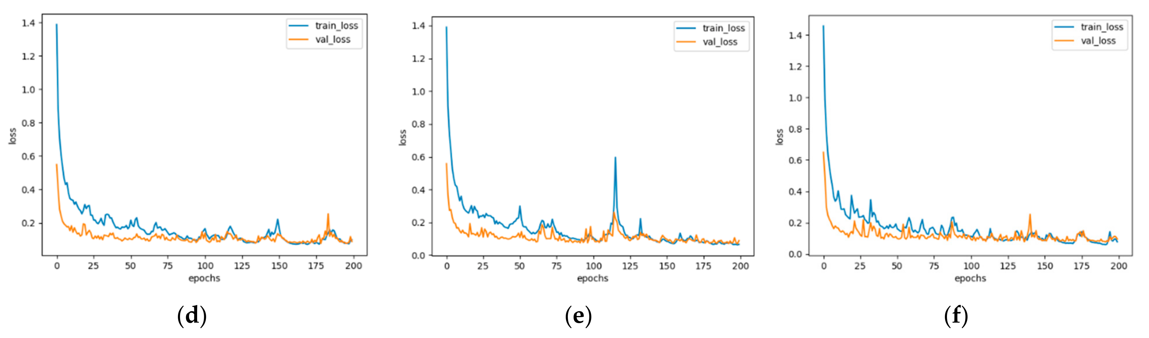
- The hybrid model adopted the same model structure as the standalone LSTM (avoiding overfitting and underfitting), with variations in input variables only. The hybrid models were executed ten times on each sub-basin, and the average value was taken.
4. Results and Discussion
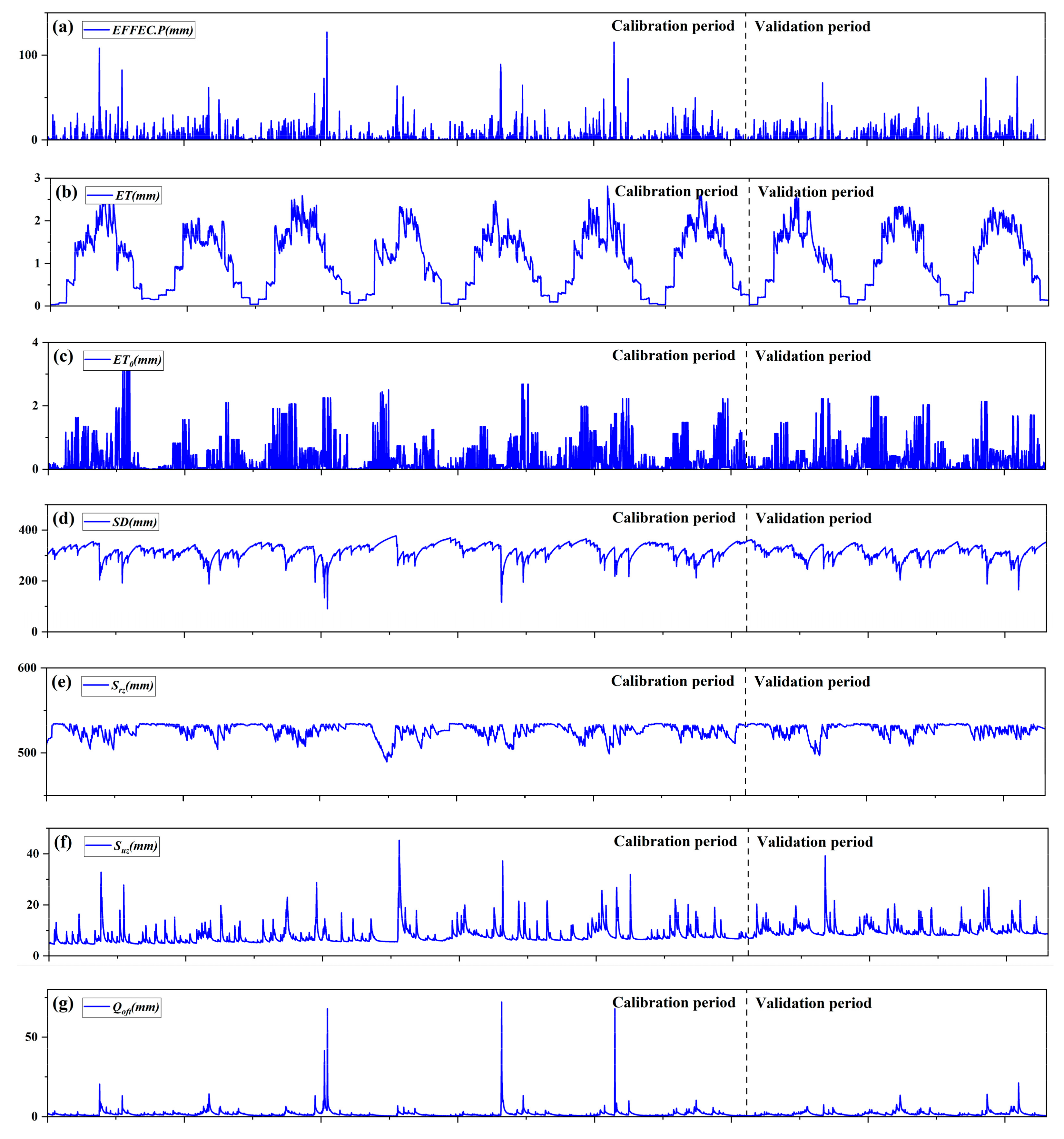
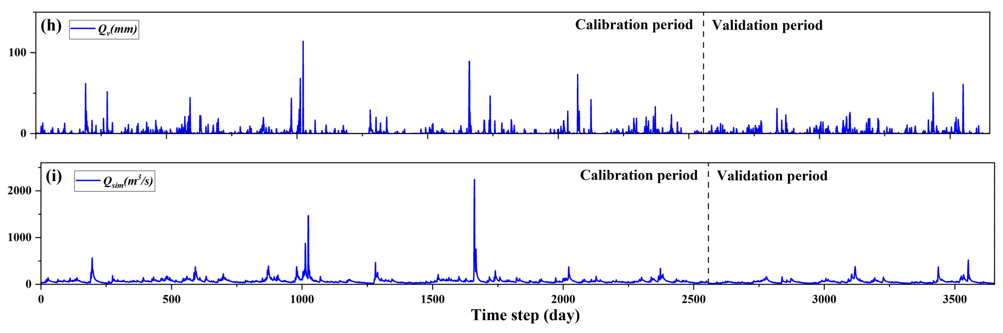
4.1. BTOP Model Simulation
4.2. Feature Dimensionality Reduction Results
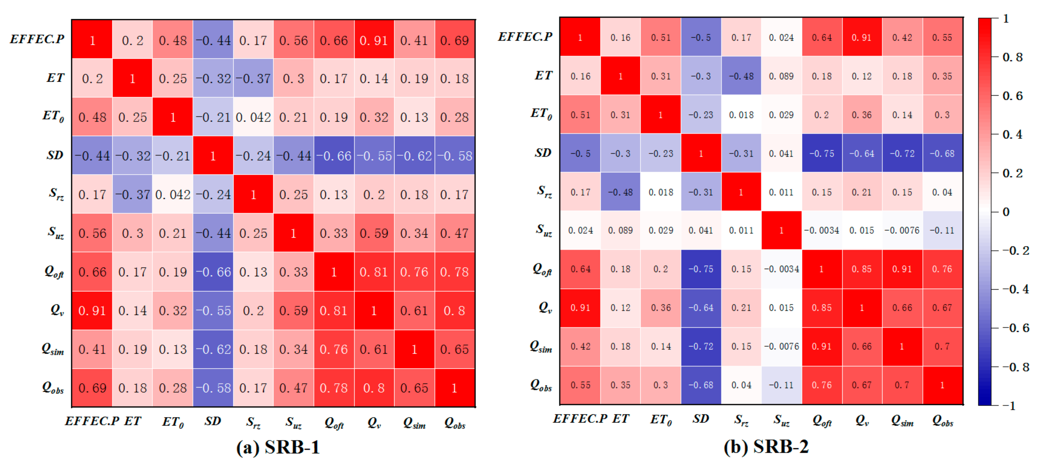
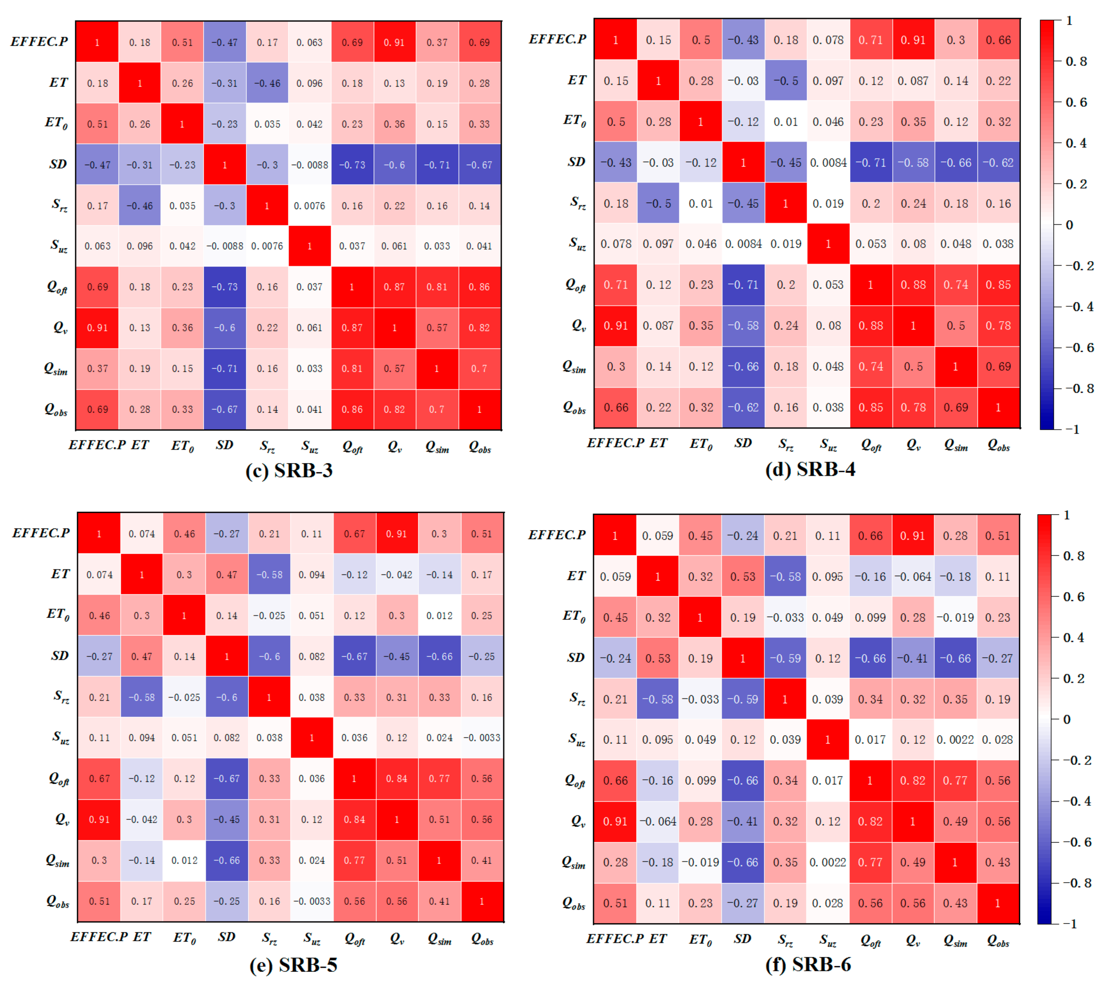
4.2.1. Feature Selection (PCC)
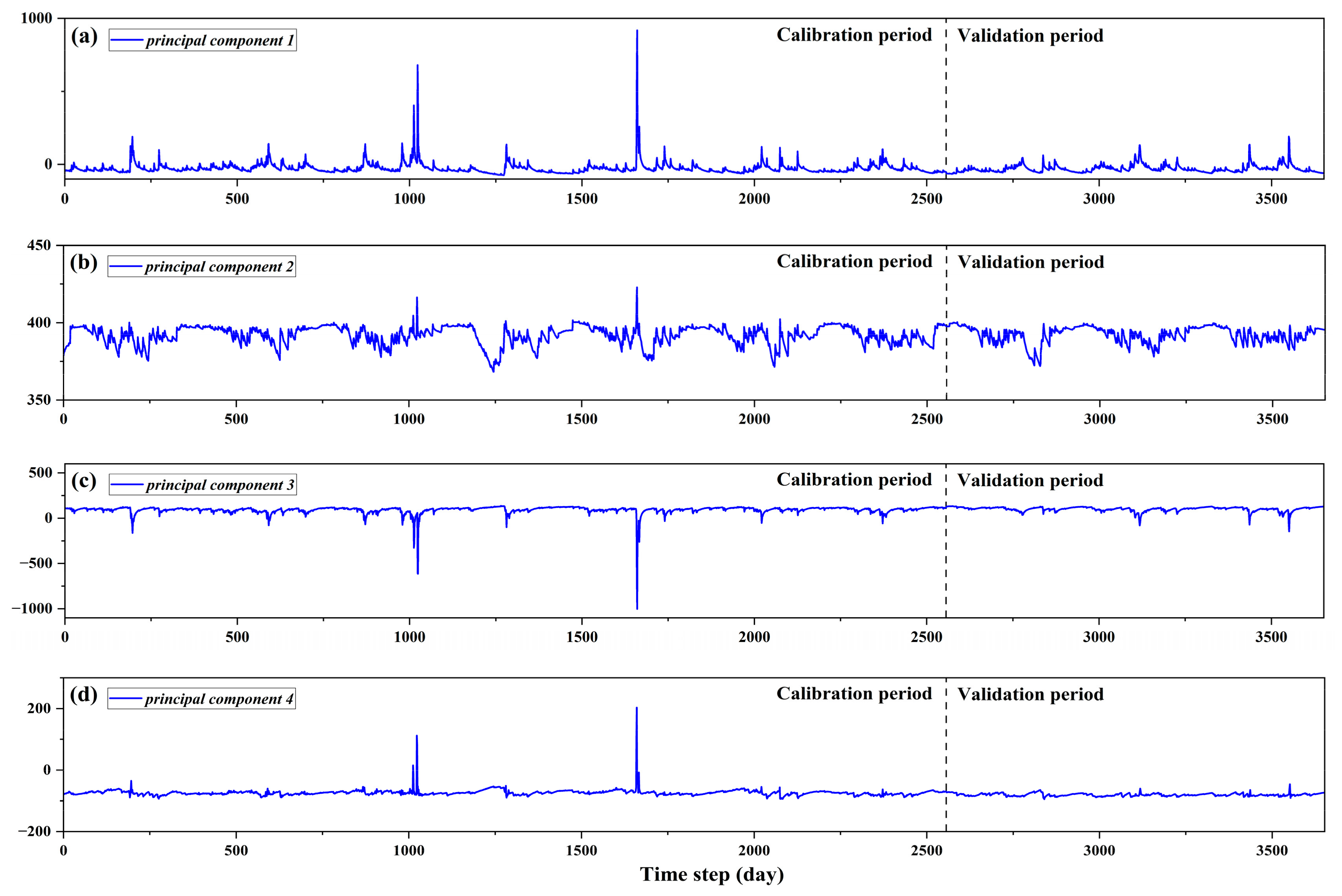
4.2.2. Feature Extraction (PCA)
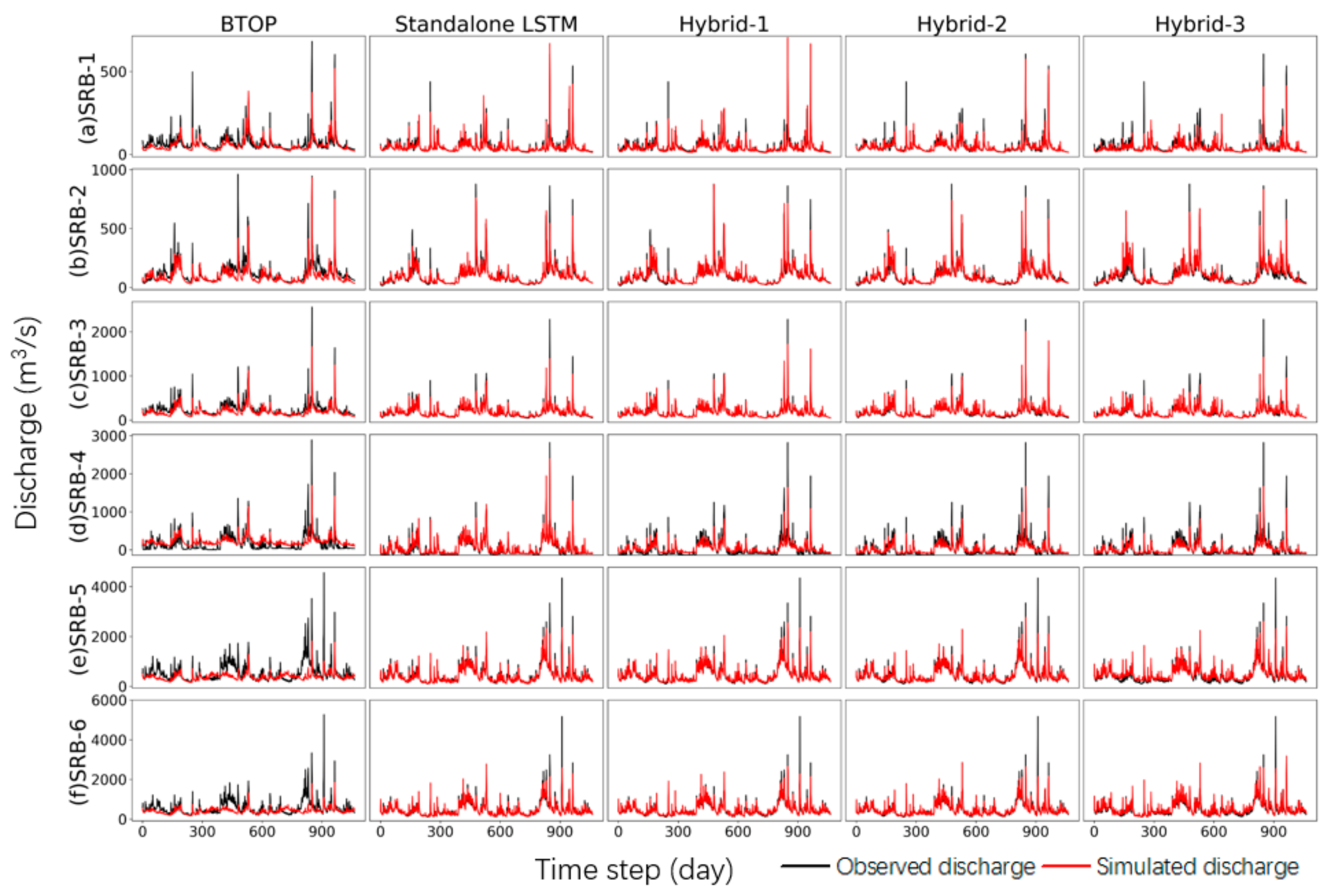
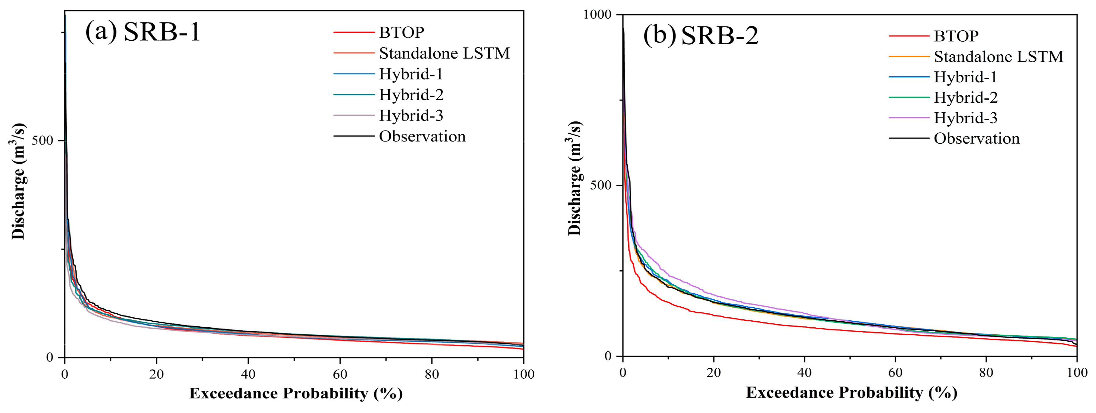
4.3. Comparison of Performance between Varied Models
5. Conclusions
- (1)
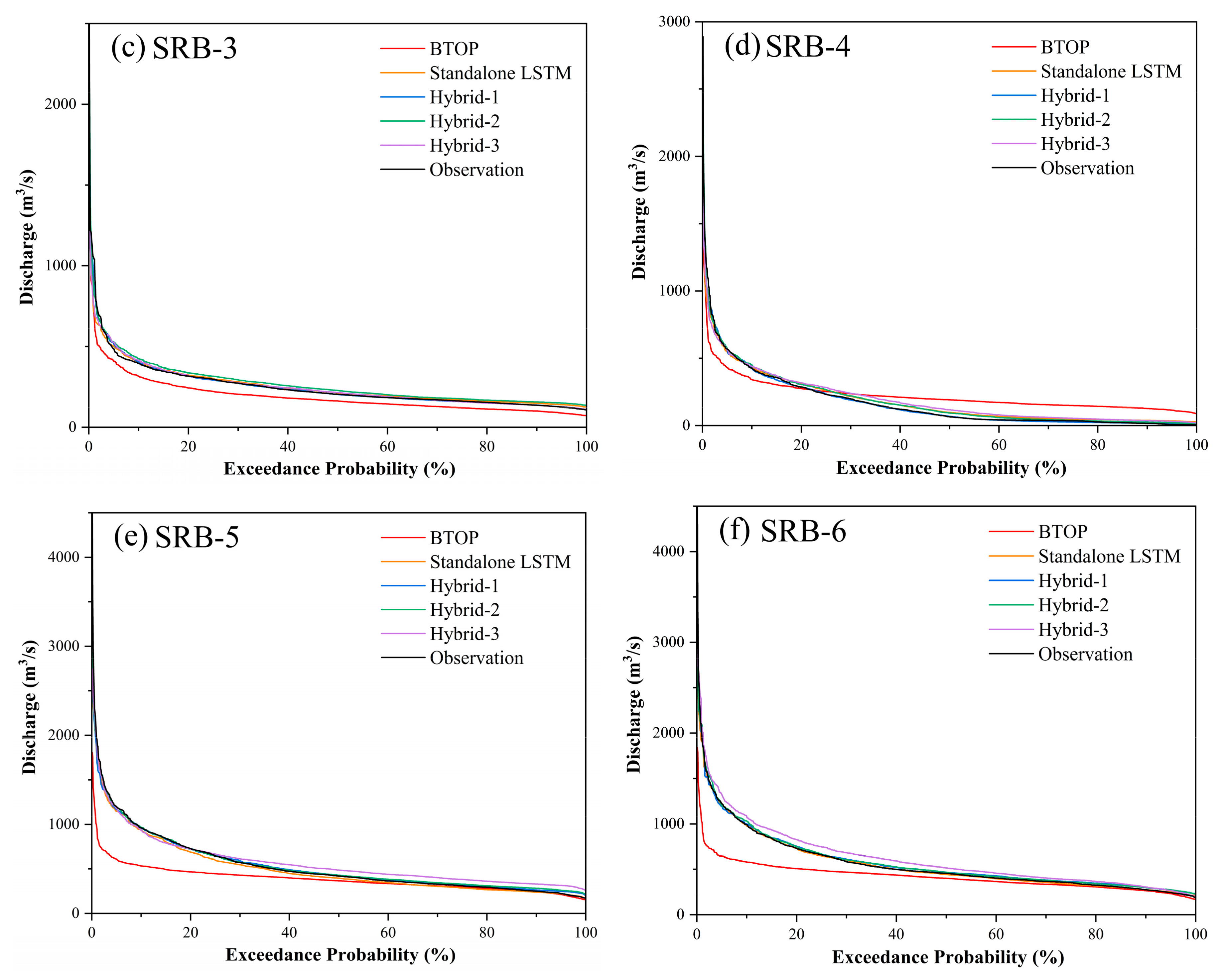
- The data-driven LSTM demonstrated superior and more stable simulation performance compared to the process-based BTOP model. The BTOP model failed to simulate two downstream basins with NSE of only 0.15 and 0.17. On the contrary, LSTM performed well across the basin, with NSE values all exceeding 0.70. Moreover, the BTOP model significantly underestimated the discharge of the six sub-basins, while the flow duration curve simulated by LSTM fitted well with that of the observed discharge.
- (2)
- Feeding the output variables from the BTOP model into LSTM as input features could provide LSTM with more physical information for learning, thereby improving simulation accuracy. Hybrid-1 and Hybrid-2 displayed comparable performances throughout the basin, both outperforming the standalone LSTM. Moreover, the exceedance probability shows that the fit of the flow duration curve of Hybrid-1 and Hybrid-2 was better than that of the standalone LSTM, and the main error of the two hybrid models originates from the slight underestimation of high flow.
- (3)
- The feature selection method, PCC, and the feature extraction method, PCA, can effectively eliminate noise within the hydrological sequences. Feeding all the BTOP model estimates into LSTM (Hybrid-3) does not enhance simulation performance but instead leads to poor simulation accuracy due to redundant and irrelevant information. Notably, Hybrid-3 exhibited overestimation behavior in the mid-flow, resulting in model accuracy far lower than Hybrid-1 and Hybrid-2 and even lower than the standalone LSTM. It is confirmed that implementing the feature dimension reduction method before constructing the hybrid model is an effective strategy to improve simulation accuracy.
Author Contributions
Funding
Data Availability Statement
Acknowledgments
Conflicts of Interest
References
- Hirpa, F.A.; Salamon, P.; Alfieri, L.; Thielen-del Pozo, J.; Zsoter, E.; Pappenberger, F. The Effect of Reference Climatology on Global Flood Forecasting. J. Hydrometeorol. 2016, 17, 1131–1145. [Google Scholar] [CrossRef]
- Croley, T.E.; He, C.S. Distributed-Parameter Large Basin Runoff Model. I: Model Development. J. Hydrol. Eng. 2005, 10, 173–181. [Google Scholar] [CrossRef]
- Pagano, T.C.; Wood, A.W.; Ramos, M.-H.; Cloke, H.L.; Pappenberger, F.; Clark, M.P.; Cranston, M.; Kavetski, D.; Mathevet, T.; Sorooshian, S.; et al. Challenges of Operational River Forecasting. J. Hydrometeorol. 2014, 15, 1692–1707. [Google Scholar] [CrossRef]
- Liu, L.; Zhou, L.; Ao, T.; Liu, X.; Shu, X. Flood Hazard Analysis Based on Rainfall Fusion: A Case Study in Dazhou City, China. Remote Sens. 2022, 14, 4843. [Google Scholar] [CrossRef]
- Shan, Y.; Yan, C.; Liu, J.; Liu, C. Predicting Velocity and Turbulent Kinetic Energy inside an Emergent Phragmites Australis Canopy with Real Morphology. Environ. Fluid Mech. 2023, 23, 943–963. [Google Scholar] [CrossRef]
- Liu, C.; Shan, Y. Impact of an Emergent Model Vegetation Patch on Flow Adjustment and Velocity. Proc. Inst. Civ. Eng.-Water Manag. 2022, 175, 55–66. [Google Scholar] [CrossRef]
- Duan, Z.; Ren, Y.; Liu, X.; Lei, H.; Hua, X.; Shu, X.; Zhou, L. A Comprehensive Comparison of Data Fusion Approaches to Multi-Source Precipitation Observations: A Case Study in Sichuan Province, China. Environ. Monit. Assess. 2022, 194, 422. [Google Scholar] [CrossRef]
- Zhu, Y.; Liu, L.; Qin, F.; Zhou, L.; Zhang, X.; Chen, T.; Li, X.; Ao, T. Application of the Regression-Augmented Regionalization Approach for BTOP Model in Ungauged Basins. Water 2021, 13, 2294. [Google Scholar] [CrossRef]
- Du, J.; Yu, X.; Zhou, L.; Ren, Y.; Ao, T. Precipitation Characteristics across the Three River Headwaters Region of the Tibetan Plateau: A Comparison between Multiple Datasets. Remote Sens. 2023, 15, 2352. [Google Scholar] [CrossRef]
- Beven, K. Linking Parameters Across Scales—Subgrid Parameterizations and Scale-Dependent Hydrological Models. Hydrol. Process. 1995, 9, 507–525. [Google Scholar] [CrossRef]
- Liu, W.; Pan, J.; Ren, Y.; Wu, Z.; Wang, J. Coupling Prediction Model for Long-Term Displacements of Arch Dams Based on Long Short-Term Memory Network. Struct. Control Health Monit. 2020, 27, e2548. [Google Scholar] [CrossRef]
- Yaseen, Z.M.; El-Shafie, A.; Jaafar, O.; Afan, H.A.; Sayl, M.N. Artificial Intelligence Based Models for Stream-Flow Forecasting: 2000–2015. J. Hydrol. 2015, 530, 829–844. [Google Scholar] [CrossRef]
- Tian, P.; Lu, H.; Feng, W.; Guan, Y.; Xue, Y. Large Decrease in Streamflow and Sediment Load of Qinghai-Tibetan Plateau Driven by Future Climate Change: A Case Study in Lhasa River Basin. Catena 2020, 187, 104340. [Google Scholar] [CrossRef]
- Salvadore, E.; Bronders, J.; Batelaan, O. Hydrological Modelling of Urbanized Catchments: A Review and Future Directions. J. Hydrol. 2015, 529, 62–81. [Google Scholar] [CrossRef]
- Arnone, E.; Zoratti, V.; Formetta, G.; Bosa, S.; Petti, M. Predicting Peakflows in Mountain River Basins and Data-Scarce Areas: A Case Study in Northeastern Italy. Hydrol. Sci. J. 2023, 68, 432–447. [Google Scholar] [CrossRef]
- Gupta, H.V.; Nearing, G.S. Debates—The Future of Hydrological Sciences: A (Common) Path Forward? Using Models and Data to Learn: A Systems Theoretic Perspective on the Future of Hydrological Science. Water Resour. Res. 2014, 50, 5351–5359. [Google Scholar] [CrossRef]
- Wagener, T.; Gupta, H.V. Model Identification for Hydrological Forecasting under Uncertainty. Stoch. Environ. Res. Risk Assess. 2005, 19, 378–387. [Google Scholar] [CrossRef]
- Renard, B.; Kavetski, D.; Kuczera, G.; Thyer, M.; Franks, S.W. Understanding Predictive Uncertainty in Hydrologic Modeling: The Challenge of Identifying Input and Structural Errors. Water Resour. Res. 2010, 46, W05521. [Google Scholar] [CrossRef]
- Vache, K.B.; McDonnell, J.J. A Process-Based Rejectionist Framework for Evaluating Catchment Runoff Model Structure. Water Resour. Res. 2006, 42, W02409. [Google Scholar] [CrossRef]
- Clark, M.P.; Nijssen, B.; Lundquist, J.D.; Kavetski, D.; Rupp, D.E.; Woods, R.A.; Freer, J.E.; Gutmann, E.D.; Wood, A.W.; Brekke, L.D.; et al. A Unified Approach for Process-Based Hydrologic Modeling: 1. Modeling Concept. Water Resour. Res. 2015, 51, 2498–2514. [Google Scholar] [CrossRef]
- Clark, M.P.; Bierkens, M.F.P.; Samaniego, L.; Woods, R.A.; Uijlenhoet, R.; Bennett, K.E.; Pauwels, V.R.N.; Cai, X.; Wood, A.W.; Peters-Lidard, C.D. The Evolution of Process-Based Hydrologic Models: Historical Challenges and the Collective Quest for Physical Realism. Hydrol. Earth Syst. Sci. 2017, 21, 3427–3440. [Google Scholar] [CrossRef] [PubMed]
- Zhu, S.; Luo, X.; Yuan, X.; Xu, Z. An Improved Long Short-Term Memory Network for Streamflow Forecasting in the Upper Yangtze River. Stoch. Environ. Res. Risk Assess. 2020, 34, 1313–1329. [Google Scholar] [CrossRef]
- Nearing, G.S.; Kratzert, F.; Sampson, A.K.; Pelissier, C.S.; Klotz, D.; Frame, J.M.; Prieto, C.; Gupta, H.V. What Role Does Hydrological Science Play in the Age of Machine Learning? Water Resour. Res. 2021, 57, e2020WR028091. [Google Scholar] [CrossRef]
- Feng, D.; Liu, J.; Lawson, K.; Shen, C. Differentiable, Learnable, Regionalized Process-Based Models With Multiphysical Outputs Can Approach State-Of-The-Art Hydrologic Prediction Accuracy. Water Resour. Res. 2022, 58, e2022WR032404. [Google Scholar] [CrossRef]
- Liu, L.; Zhou, L.; Gusyev, M.; Ren, Y. Unravelling and Improving the Potential of Global Discharge Reanalysis Dataset in Streamflow Estimation in Ungauged Basins. J. Clean. Prod. 2023, 419, 138282. [Google Scholar] [CrossRef]
- Xiao, Q.; Zhou, L.; Xiang, X.; Liu, L.; Liu, X.; Li, X.; Ao, T. Integration of Hydrological Model and Time Series Model for Improving the Runoff Simulation: A Case Study on BTOP Model in Zhou River Basin, China. Appl. Sci. 2022, 12, 6883. [Google Scholar] [CrossRef]
- Hochreiter, S.; Schmidhuber, J. Long Short-Term Memory. Neural Comput. 1997, 9, 1735–1780. [Google Scholar] [CrossRef]
- Li, Q.; Wang, Z.; Shangguan, W.; Li, L.; Yao, Y.; Yu, F. Improved Daily SMAP Satellite Soil Moisture Prediction over China Using Deep Learning Model with Transfer Learning. J. Hydrol. 2021, 600, 126698. [Google Scholar] [CrossRef]
- Ahmed, A.A.M.; Deo, R.C.; Feng, Q.; Ghahramani, A.; Raj, N.; Yin, Z.; Yang, L. Hybrid Deep Learning Method for a Week-Ahead Evapotranspiration Forecasting. Stoch. Environ. Res. Risk Assess. 2022, 36, 831–849. [Google Scholar] [CrossRef]
- Kratzert, F.; Klotz, D.; Brenner, C.; Schulz, K.; Herrnegger, M. Rainfall–Runoff Modelling Using Long Short-Term Memory (LSTM) Networks. Hydrol. Earth Syst. Sci. 2018, 22, 6005–6022. [Google Scholar] [CrossRef]
- Kratzert, F.; Klotz, D.; Shalev, G.; Klambauer, G.; Hochreiter, S.; Nearing, G. Towards Learning Universal, Regional, and Local Hydrological Behaviors via Machine Learning Applied to Large-Sample Datasets. Hydrol. Earth Syst. Sci. 2019, 23, 5089–5110. [Google Scholar] [CrossRef]
- Tian, Y.; Xu, Y.-P.; Yang, Z.; Wang, G.; Zhu, Q. Integration of a Parsimonious Hydrological Model with Recurrent Neural Networks for Improved Streamflow Forecasting. Water 2018, 10, 1655. [Google Scholar] [CrossRef]
- Xiang, Z.; Yan, J.; Demir, I. A Rainfall-Runoff Model With LSTM-Based Sequence-to-Sequence Learning. Water Resour. Res. 2020, 56, e2019WR025326. [Google Scholar] [CrossRef]
- Tsai, W.-P.; Feng, D.; Pan, M.; Beck, H.; Lawson, K.; Yang, Y.; Liu, J.; Shen, C. From Calibration to Parameter Learning: Harnessing the Scaling Effects of Big Data in Geoscientific Modeling. Nat. Commun. 2021, 12, 5988. [Google Scholar] [CrossRef]
- Lu, D.; Konapala, G.; Painter, S.L.; Kao, S.-C.; Gangrade, S. Streamflow Simulation in Data-Scarce Basins Using Bayesian and Physics-Informed Machine Learning Models. J. Hydrometeorol. 2021, 22, 1421–1438. [Google Scholar] [CrossRef]
- Konapala, G.; Kao, S.-C.; Painter, S.L.; Lu, D. Machine Learning Assisted Hybrid Models Can Improve Streamflow Simulation in Diverse Catchments across the Conterminous US. Environ. Res. Lett. 2020, 15, 104022. [Google Scholar] [CrossRef]
- Wi, S.; Steinschneider, S. Assessing the Physical Realism of Deep Learning Hydrologic Model Projections Under Climate Change. Water Resour. Res. 2022, 58, e2022WR032123. [Google Scholar] [CrossRef]
- Saeys, Y.; Inza, I.; Larrañaga, P. A Review of Feature Selection Techniques in Bioinformatics. Bioinformatics 2007, 23, 2507–2517. [Google Scholar] [CrossRef]
- Zhang, D.; Chen, S.; Zhou, Z.-H. Constraint Score: A New Filter Method for Feature Selection with Pairwise Constraints. Pattern Recognit. 2008, 41, 1440–1451. [Google Scholar] [CrossRef]
- Wang, J.; Wu, L.; Kong, J.; Li, Y.; Zhang, B. Maximum Weight and Minimum Redundancy: A Novel Framework for Feature Subset Selection. Pattern Recognit. 2013, 46, 1616–1627. [Google Scholar] [CrossRef]
- Lin, S.-S.; Zhang, N.; Zhou, A.; Shen, S.-L. Time-Series Prediction of Shield Movement Performance during Tunneling Based on Hybrid Model. Tunn. Undergr. Space Technol. 2022, 119, 104245. [Google Scholar] [CrossRef]
- Pathy, A.; Meher, S.; Balasubramanian, P. Predicting Algal Biochar Yield Using eXtreme Gradient Boosting (XGB) Algorithm of Machine Learning Methods. Algal Res. 2020, 50, 102006. [Google Scholar] [CrossRef]
- Chen, H.; Chang, X. Photovoltaic Power Prediction of LSTM Model Based on Pearson Feature Selection. Energy Rep. 2021, 7, 1047–1054. [Google Scholar] [CrossRef]
- Xie, A.; Yang, H.; Chen, J.; Sheng, L.; Zhang, Q. A Short-Term Wind Speed Forecasting Model Based on a Multi-Variable Long Short-Term Memory Network. Atmosphere 2021, 12, 651. [Google Scholar] [CrossRef]
- Yang, J.; Zhang, D.; Frangi, A.F.; Yang, J. Two-Dimensional PCA: A New Approach to Appearance-Based Face Representation and Recognition. IEEE Trans. Pattern Anal. Mach. Intell. 2004, 26, 131–137. [Google Scholar] [CrossRef]
- Zhang, Y.; Yan, B.; Aasma, M. A Novel Deep Learning Framework: Prediction and Analysis of Financial Time Series Using CEEMD and LSTM. Expert Syst. Appl. 2020, 159, 113609. [Google Scholar] [CrossRef]
- Xu, W.; Liu, P.; Cheng, L.; Zhou, Y.; Xia, Q.; Gong, Y.; Liu, Y. Multi-Step Wind Speed Prediction by Combining a WRF Simulation and an Error Correction Strategy. Renew. Energy 2021, 163, 772–782. [Google Scholar] [CrossRef]
- Zhang, J.; Chen, X.; Khan, A.; Zhang, Y.; Kuang, X.; Liang, X.; Taccari, M.L.; Nuttall, J. Daily Runoff Forecasting by Deep Recursive Neural Network. J. Hydrol. 2021, 596, 126067. [Google Scholar] [CrossRef]
- Martens, B.; Miralles, D.G.; Lievens, H.; van der Schalie, R.; de Jeu, R.A.M.; Fernandez-Prieto, D.; Beck, H.E.; Dorigo, W.A.; Verhoest, N.E.C. GLEAM v3: Satellite-Based Land Evaporation and Root-Zone Soil Moisture. Geosci. Model Dev. 2017, 10, 1903–1925. [Google Scholar] [CrossRef]
- Yamazaki, D.; Ikeshima, D.; Tawatari, R.; Yamaguchi, T.; O’Loughlin, F.; Neal, J.C.; Sampson, C.C.; Kanae, S.; Bates, P.D. A High-Accuracy Map of Global Terrain Elevations. Geophys. Res. Lett. 2017, 44, 5844–5853. [Google Scholar] [CrossRef]
- The Potential Evapotranspiration (EP) from the Climatic Research Unit (CRU) of the School of Environmental Sciences (ENV) at the University of East Anglia (UEA). Available online: http://www.cru.uea.ac.uk/ (accessed on 25 March 2022).
- The Leaf Area Index (LAI) of the National Centers for Environmental Information. Available online: https://www.ncei.noaa.gov/Data/Avhrr-Land-Leaf-Area-Index-and-Fapar/Access/ (accessed on 25 March 2022).
- FAO Digital Soil Map of the World (DSMW). Available online: http://www.fao.org/Land-Water/Land/Land-Governance/Landresources-Planning-Toolbox/Category/Details/En/c/1026564/ (accessed on 25 March 2022).
- LP DAAC-MCD12Q1. Available online: https://lpdaac.usgs.gov/Products/Mcd12q1v006/ (accessed on 25 March 2022).
- Takeuchi, K.; Ao, T.Q.; Ishidaira, H. Introduction of Block-Wise Use of TOPMODEL and Muskingum-Cunge Method for the Hydro-Environmental Simulation of a Large Ungauged Basin. Hydrol. Sci. J.-J. Sci. Hydrol. 1999, 44, 633–646. [Google Scholar] [CrossRef]
- Ao, T.; Ishidaira, H.; Takeuchi, K. Study of Distributed Runoff Simulation Model Based on Block Type Topmodel and Muskingum-Cunge Method. Proc. Hydraul. Eng. 1999, 43, 7–12. [Google Scholar] [CrossRef]
- Takeuchi, K.; Hapuarachchi, P.; Zhou, M.; Ishidaira, H.; Magome, J. A BTOP Model to Extend TOPMODEL for Distributed Hydrological Simulation of Large Basins. Hydrol. Process. 2008, 22, 3236–3251. [Google Scholar] [CrossRef]
- Zhou, M.C.; Ishidaira, H.; Hapuarachchi, H.P.; Magome, J.; Kiem, A.S.; Takeuchi, K. Estimating Potential Evapotranspiration Using Shuttleworth-Wallace Model and NOAA-AVHRR NDVI Data to Feed a Distributed Hydrological Model over the Mekong River Basin. J. Hydrol. 2006, 327, 151–173. [Google Scholar] [CrossRef]
- Beven, K.J.; Kirkby, M.J.; Freer, J.E.; Lamb, R. A History of TOPMODEL. Hydrol. Earth Syst. Sci. 2021, 25, 527–549. [Google Scholar] [CrossRef]
- Barry, D.; Bajracharya, K. On the Muskingum-Cunge Flood Routing Method. Environ. Int. 1995, 21, 485–490. [Google Scholar] [CrossRef]
- Navarathinam, K.; Gusyev, M.A.; Hasegawa, A.; Magome, J.; Takeuchi, K. Agricultural Flood and Drought Risk Reduction by a Proposed Multi-Purpose Dam: A Case Study of the Malwathoya River Basin, Sri Lanka. In Proceedings of the 21st International Congress on Modelling and Simulation (MODSIM 2015), Queensland, Australia, 29 November–4 December 2015; Weber, T., McPhee, M.J., Anderssen, R.S., Eds.; Modelling & Simulation Soc Australia & New Zealand Inc.: Christchurch, New Zealand, 2015; pp. 1600–1606. [Google Scholar]
- Ishidaira, H.; Sawada, H.; Masumoto, T. Studies on the Mekong and River Basin-Modelling of Hydrology Water Resources. Hydrol. Process. 2008, 22, 1243–1245. [Google Scholar] [CrossRef]
- Hapuarachchi, H.A.P.; Takeuchi, K.; Zhou, M.; Kiem, A.S.; Georgievski, M.; Magome, J.; Ishidaira, H. Investigation of the Mekong River Basin Hydrology for 1980-2000 Using the YHyM. Hydrol. Process. 2008, 22, 1246–1256. [Google Scholar] [CrossRef]
- Liu, L.; Zhou, L.; Li, X.; Chen, T.; Ao, T. Screening and Optimizing the Sensitive Parameters of BTOPMC Model Based on UQ-PyL Software: Case Study of a Flood Event in the Fuji River Basin, Japan. J. Hydrol. Eng. 2020, 25, 05020030. [Google Scholar] [CrossRef]
- Zhou, L.; Rasmy, M.; Takeuchi, K.; Koike, T.; Selvarajah, H.; Ao, T. Adequacy of Near Real-Time Satellite Precipitation Products in Driving Flood Discharge Simulation in the Fuji River Basin, Japan. Appl. Sci. 2021, 11, 1087. [Google Scholar] [CrossRef]
- Zhou, L.; Koike, T.; Takeuchi, K.; Rasmy, M.; Onuma, K.; Ito, H.; Selvarajah, H.; Liu, L.; Li, X.; Ao, T. A Study on Availability of Ground Observations and Its Impacts on Bias Correction of Satellite Precipitation Products and Hydrologic Simulation Efficiency. J. Hydrol. 2022, 610, 127595. [Google Scholar] [CrossRef]
- Liu, L.; Ao, T.; Zhou, L.; Takeuchi, K.; Gusyev, M.; Zhang, X.; Wang, W.; Ren, Y. Comprehensive Evaluation of Parameter Importance and Optimization Based on the Integrated Sensitivity Analysis System: A Case Study of the BTOP Model in the Upper Min River Basin, China. J. Hydrol. 2022, 610, 127819. [Google Scholar] [CrossRef]
- Duan, Q.; Sorooshian, S.; Gupta, V. Effective and Efficient Global Optimization for Conceptual Rainfall-Runoff Models. Water Resour. Res. 1992, 28, 1015–1031. [Google Scholar] [CrossRef]
- Hochreiter, S.; Schmidhuber, J. LSTM Can Solve Hard Long Time Lag Problems. In Advances in Neural Information Processing Systems 9: Proceedings of the 1996 Conference; Mozer, M.C., Jordan, M.I., Petsche, T., Eds.; Advances in Neural Information Processing Systems; M I T Press: Cambridge, UK, 1997; Volume 9, pp. 473–479. [Google Scholar]
- Yang, S.; Yu, X.; Zhou, Y. LSTM and GRU Neural Network Performance Comparison Study: Taking Yelp Review Dataset as an Example. In 2020 International Workshop on Electronic Communication and Artificial Intelligence (IWECAI); IEEE: Shanghai, China, 2020; pp. 98–101. [Google Scholar] [CrossRef]
- Yu, Y.; Si, X.; Hu, C.; Zhang, J. A Review of Recurrent Neural Networks: LSTM Cells and Network Architectures. Neural Comput. 2019, 31, 1235–1270. [Google Scholar] [CrossRef]
- Zhang, Z.; Qin, H.; Liu, Y.; Wang, Y.; Yao, L.; Li, Q.; Li, J.; Pei, S. Long Short-Term Memory Network Based on Neighborhood Gates for Processing Complex Causality in Wind Speed Prediction. Energy Convers. Manag. 2019, 192, 37–51. [Google Scholar] [CrossRef]
- Karl Pearson, F.R.S. LIII. On Lines and Planes of Closest Fit to Systems of Points in Space. Lond. Edinb. Dublin Philos. Mag. J. Sci. 2010, 2, 559–572. Available online: https://www.tandfonline.com/doi/abs/10.1080/14786440109462720 (accessed on 26 July 2023). [CrossRef]
- Hotelling, H. Analysis of a Complex of Statistical Variables into Principal Components. J. Educ. Psychol. 1933, 24, 417–441. [Google Scholar] [CrossRef]
- Cui, W.; Zhang, Y.; Zhang, X.; Li, L.; Liou, F. Metal Additive Manufacturing Parts Inspection Using Convolutional Neural Network. Appl. Sci. 2020, 10, 545. [Google Scholar] [CrossRef]
- Hood, M.J.; Clausen, J.C.; Warner, G.S. Comparison of Stormwater Lag Times for Low Impact and Traditional Residential Development. J. Am. Water Resour. Assoc. 2007, 43, 1036–1046. [Google Scholar] [CrossRef]
- Mao, G.; Wang, M.; Liu, J.; Wang, Z.; Wang, K.; Meng, Y.; Zhong, R.; Wang, H.; Li, Y. Comprehensive Comparison of Artificial Neural Networks and Long Short-Term Memory Networks for Rainfall-Runoff Simulation. Phys. Chem. Earth Parts ABC 2021, 123, 103026. [Google Scholar] [CrossRef]
- Yu, Q.; Jiang, L.; Wang, Y.; Liu, J. Enhancing Streamflow Simulation Using Hybridized Machine Learning Models in a Semi-Arid Basin of the Chinese Loess Plateau. J. Hydrol. 2023, 617, 129115. [Google Scholar] [CrossRef]
- Lei, H.; Zhao, H.; Ao, T.; Hu, W. Quantifying the Reliability and Uncertainty of Satellite, Reanalysis, and Merged Precipitation Products in Hydrological Simulations over the Topographically Diverse Basin in Southwest China. Remote Sens. 2022, 15, 213. [Google Scholar] [CrossRef]

| Variable | Unit | Description |
|---|---|---|
| Effec.P | mm | Net precipitation |
| ET | mm | Actual evaporation |
| ET0 | mm | Actual interception evapotranspiration |
| SD | mm | The soil moisture saturation deficit |
| Srz | mm | The root zone water storage |
| Suz | mm | The unsaturated zone water storage |
| Qoft | mm | Flow generation flux, the sum of simulated Hortonian overland flow flux, saturation excess runoff flux and groundwater flux |
| Qv | mm | Groundwater recharge flux |
| Sub- Basin | Calibration Period | Validation Period | ||||||
|---|---|---|---|---|---|---|---|---|
| MAE (m3/s) | RMSE (m3/s) | NSE | PCC | MAE (m3/s) | RMSE (m3/s) | NSE | PCC | |
| SRB-1 | 19.62 | 37.54 | 0.77 | 0.89 | 19.01 | 31.19 | 0.63 | 0.82 |
| SRB-2 | 37.15 | 64.72 | 0.56 | 0.81 | 33.79 | 53.07 | 0.66 | 0.88 |
| SRB-3 | 63.79 | 103.09 | 0.70 | 0.89 | 62.34 | 94.72 | 0.66 | 0.89 |
| SRB-4 | 125.31 | 155.40 | 0.65 | 0.85 | 125.34 | 155.81 | 0.55 | 0.82 |
| SRB-5 | 205.73 | 324.06 | 0.14 | 0.54 | 199.18 | 340.60 | 0.15 | 0.59 |
| SRB-6 | 210.34 | 338.52 | 0.19 | 0.54 | 192.25 | 333.84 | 0.17 | 0.59 |
| Sub-Basin | Lag Time (day) | Effec.P | ET | ET0 | SD | Srz | Suz | Qoft | Qv |
|---|---|---|---|---|---|---|---|---|---|
| SRB-1 | 0 | 0.43 ** | 0.19 ** | 0.19 ** | −0.58 ** | 0.17 ** | 0.43 ** | 0.71 ** | 0.60 ** |
| 1 | 0.69 ** | 0.18 ** | 0.28 ** | −0.58 ** | 0.17 ** | 0.47 ** | 0.78 ** | 0.80 ** | |
| 2 | 0.37 ** | 0.16 ** | 0.20 ** | −0.38 ** | 0.11 ** | 0.34 ** | 0.37 ** | 0.39 ** | |
| SRB-2 | 0 | 0.41 ** | 0.35 ** | 0.24 ** | −0.68 ** | 0.05 * | −0.11 * | 0.72 ** | 0.54 ** |
| 1 | 0.55 ** | 0.35 ** | 0.30 ** | −0.67 ** | 0.04 * | 0.11 ** | 0.76 ** | 0.67 ** | |
| 2 | 0.35 ** | 0.22 ** | 0.33 ** | −0.54 ** | 0.01 | −0.12 ** | 0.51 ** | 0.42 ** | |
| SRB-3 | 0 | 0.36 ** | 0.28 ** | 0.20 ** | −0.64 ** | 0.14 ** | 0.04 | 0.67 ** | 0.51 ** |
| 1 | 0. 69 ** | 0.28 ** | 0.33 ** | −0.67 ** | 0.14 ** | 0.04 * | 0.86 ** | 0.82 ** | |
| 2 | 0.41 ** | 0.26 ** | 0.25 ** | −0.49 ** | 0.09 ** | 0.02 | 0.45 ** | 0.46 ** | |
| SRB-4 | 0 | 0.24 ** | 0.22 ** | 0.17 ** | −0.55 ** | 0.15 ** | 0.03 | 0.57 ** | 0.41 ** |
| 1 | 0.66 ** | 0.22 ** | 0.31 ** | −0.62 ** | 0.16 ** | 0.04 | 0.85 ** | 0.78 ** | |
| 2 | 0.43 ** | 0.20 ** | 0.26 ** | −0.45 ** | 0.11 ** | 0.01 | 0.55 ** | 0.50 ** | |
| SRB-5 | 0 | 0.20 ** | 0.18 ** | 0.13 ** | −0.23 ** | 0.16 ** | −0.01 | 0.36 ** | 0.31 ** |
| 1 | 0.51 ** | 0.17 ** | 0.25 ** | −0.25 ** | 0.16 ** | −0.01 | 0.56 ** | 0.56 ** | |
| 2 | 0.30 ** | 0.15 ** | 0.20 ** | −0.15 ** | 0.12 ** | −0.04 | 0.32 ** | 0.32 ** | |
| SRB-6 | 0 | 0.19 ** | 0.12 ** | 0.11 ** | −0.25 ** | 0.19 ** | 0.02 | 0.36 ** | 0.30 ** |
| 1 | 0.50 ** | 0.11 ** | 0.23 ** | −0.27 ** | 0.19 ** | 0.03 | 0.56 ** | 0.56 * | |
| 2 | 0.30 ** | 0.09 ** | 0.18 ** | −0.18 ** | 0.15 ** | −0.01 | 0.34 ** | 0.33 ** |
| SRB-1 | SRB-2 | SRB-3 | ||||
| Ingredient | Eigenvalues | Cumulative (%) | Eigenvalues | Cumulative (%) | Eigenvalues | Cumulative (%) |
| 1 | 4.207 | 46.740 | 4.146 | 46.063 | 4.059 | 45.102 |
| 2 | 1.395 | 62.240 | 1.534 | 63.107 | 1.485 | 61.598 |
| 3 | 1.138 | 74.882 | 1.102 | 75.353 | 1.122 | 74.068 |
| 4 | 1.002 | 83.873 | 1.001 | 86.445 | 1.003 | 85.143 |
| 5 | 0.560 | 91.172 | 0.596 | 93.102 | 0.621 | 92.048 |
| 6 | 0.297 | 94.773 | 0.378 | 97.303 | 0.407 | 96.635 |
| 7 | 0.227 | 98.069 | 0.169 | 99.178 | 0.190 | 98.743 |
| 8 | 0.130 | 99.516 | 0.049 | 99.720 | 0.077 | 99.604 |
| 9 | 0.044 | 100.000 | 0.025 | 100.000 | 0.036 | 100.000 |
| SRB-4 | SRB-5 | SRB-6 | ||||
| Ingredient | Eigenvalues | Cumulative (%) | Eigenvalues | Cumulative (%) | Eigenvalues | Cumulative (%) |
| 1 | 3.918 | 43.537 | 3.413 | 42.368 | 3.487 | 42.078 |
| 2 | 1.592 | 61.222 | 1.955 | 64.086 | 2.005 | 64.352 |
| 3 | 1.139 | 73.879 | 1.672 | 75.085 | 1.554 | 75.361 |
| 4 | 1.007 | 84.885 | 1.004 | 85.857 | 1.072 | 85.897 |
| 5 | 0.605 | 91.798 | 0.416 | 92.239 | 0.381 | 92.285 |
| 6 | 0.395 | 96.184 | 0.236 | 95.905 | 0.235 | 95.916 |
| 7 | 0.224 | 98.674 | 0.172 | 98.531 | 0.133 | 98.528 |
| 8 | 0.084 | 99.603 | 0.092 | 99.549 | 0.092 | 99.546 |
| 9 | 0.036 | 100.000 | 0.041 | 100.000 | 0.041 | 100.000 |
| Sub-Basin Number | Metrics | BTOP | Standalone LSTM | Hybrid-1 | Hybrid-2 | Hybrid-3 |
|---|---|---|---|---|---|---|
| SRB-1 | MAE (m3/s) | 18.95 | 10.50 | 11.96 | 10.50 | 15.06 |
| RMSE (m3/s) | 31.43 | 26.92 | 25.95 | 25.01 | 31.78 | |
| NSE | 0.63 | 0.73 | 0.75 | 0.76 | 0.64 | |
| PCC | 0.83 | 0.86 | 0.88 | 0.89 | 0.85 | |
| SRB-2 | MAE (m3/s) | 34.59 | 18.80 | 18.38 | 19.17 | 26.01 |
| RMSE (m3/s) | 53.82 | 46.02 | 40.80 | 41.62 | 45.52 | |
| NSE | 0.66 | 0.75 | 0.80 | 0.80 | 0.76 | |
| PCC | 0.88 | 0.87 | 0.90 | 0.90 | 0.89 | |
| SRB-3 | MAE (m3/s) | 63.29 | 32.75 | 29.75 | 36.74 | 36.23 |
| RMSE (m3/s) | 95.95 | 68.19 | 61.84 | 61.07 | 74.19 | |
| NSE | 0.66 | 0.83 | 0.86 | 0.86 | 0.80 | |
| PCC | 0.90 | 0.92 | 0.93 | 0.94 | 0.90 | |
| SRB-4 | MAE (m3/s) | 126.09 | 48.51 | 37.82 | 44.17 | 54.02 |
| RMSE (m3/s) | 157.14 | 77.96 | 69.60 | 72.58 | 84.39 | |
| NSE | 0.55 | 0.89 | 0.91 | 0.90 | 0.87 | |
| PCC | 0.81 | 0.95 | 0.96 | 0.95 | 0.94 | |
| SRB-5 | MAE (m3/s) | 203.60 | 71.50 | 67.43 | 73.54 | 103.70 |
| RMSE (m3/s) | 345.39 | 157.43 | 152.89 | 151.74 | 165.59 | |
| NSE | 0.15 | 0.82 | 0.83 | 0.84 | 0.80 | |
| PCC | 0.62 | 0.92 | 0.92 | 0.92 | 0.91 | |
| SRB-6 | MAE (m3/s) | 196.34 | 81.87 | 75.66 | 81.41 | 112.22 |
| RMSE (m3/s) | 338.47 | 184.85 | 167.10 | 168.24 | 196.35 | |
| NSE | 0.17 | 0.75 | 0.80 | 0.79 | 0.72 | |
| PCC | 0.62 | 0.88 | 0.90 | 0.90 | 0.88 |
Disclaimer/Publisher’s Note: The statements, opinions and data contained in all publications are solely those of the individual author(s) and contributor(s) and not of MDPI and/or the editor(s). MDPI and/or the editor(s) disclaim responsibility for any injury to people or property resulting from any ideas, methods, instructions or products referred to in the content. |
© 2023 by the authors. Licensee MDPI, Basel, Switzerland. This article is an open access article distributed under the terms and conditions of the Creative Commons Attribution (CC BY) license (https://creativecommons.org/licenses/by/4.0/).
Share and Cite
Nimai, S.; Ren, Y.; Ao, T.; Zhou, L.; Liang, H.; Cui, Y. Enhancing Runoff Simulation Using BTOP-LSTM Hybrid Model in the Shinano River Basin. Water 2023, 15, 3758. https://doi.org/10.3390/w15213758
Nimai S, Ren Y, Ao T, Zhou L, Liang H, Cui Y. Enhancing Runoff Simulation Using BTOP-LSTM Hybrid Model in the Shinano River Basin. Water. 2023; 15(21):3758. https://doi.org/10.3390/w15213758
Chicago/Turabian StyleNimai, Silang, Yufeng Ren, Tianqi Ao, Li Zhou, Hanxu Liang, and Yanmin Cui. 2023. "Enhancing Runoff Simulation Using BTOP-LSTM Hybrid Model in the Shinano River Basin" Water 15, no. 21: 3758. https://doi.org/10.3390/w15213758
APA StyleNimai, S., Ren, Y., Ao, T., Zhou, L., Liang, H., & Cui, Y. (2023). Enhancing Runoff Simulation Using BTOP-LSTM Hybrid Model in the Shinano River Basin. Water, 15(21), 3758. https://doi.org/10.3390/w15213758