
2D and 3D Numerical Simulation of Dam-Break Flooding: A Case Study of the Tuzluca Dam, Turkey


Abstract
:1. Introduction
2. Materials and Methods
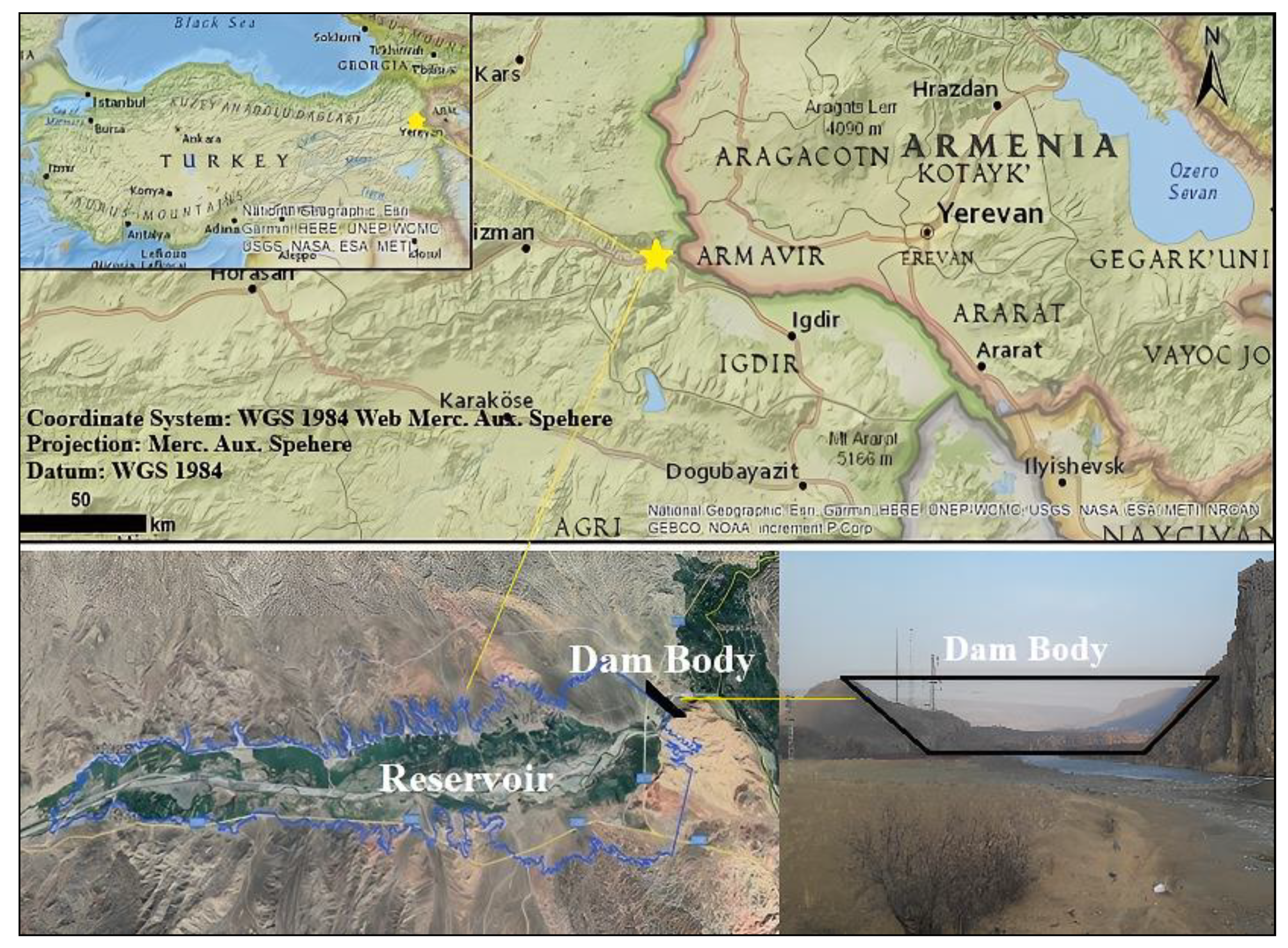
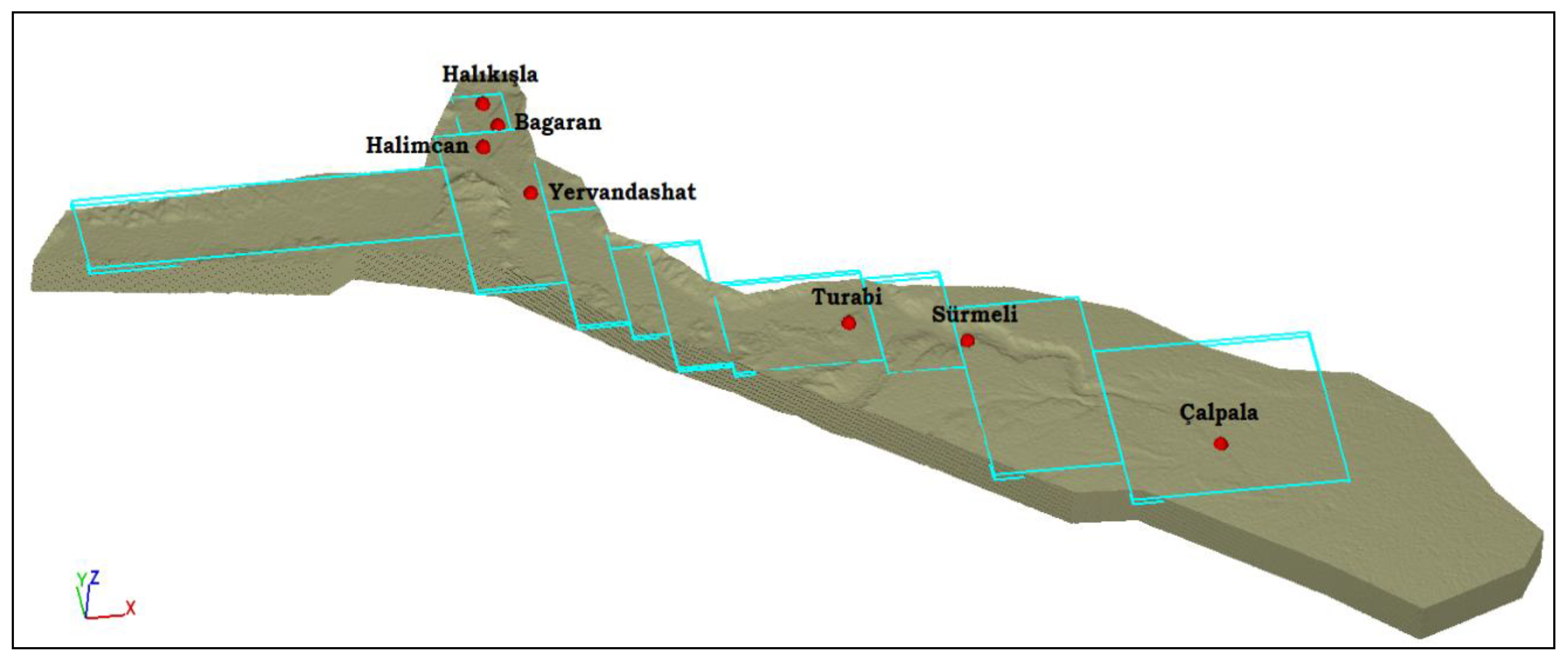
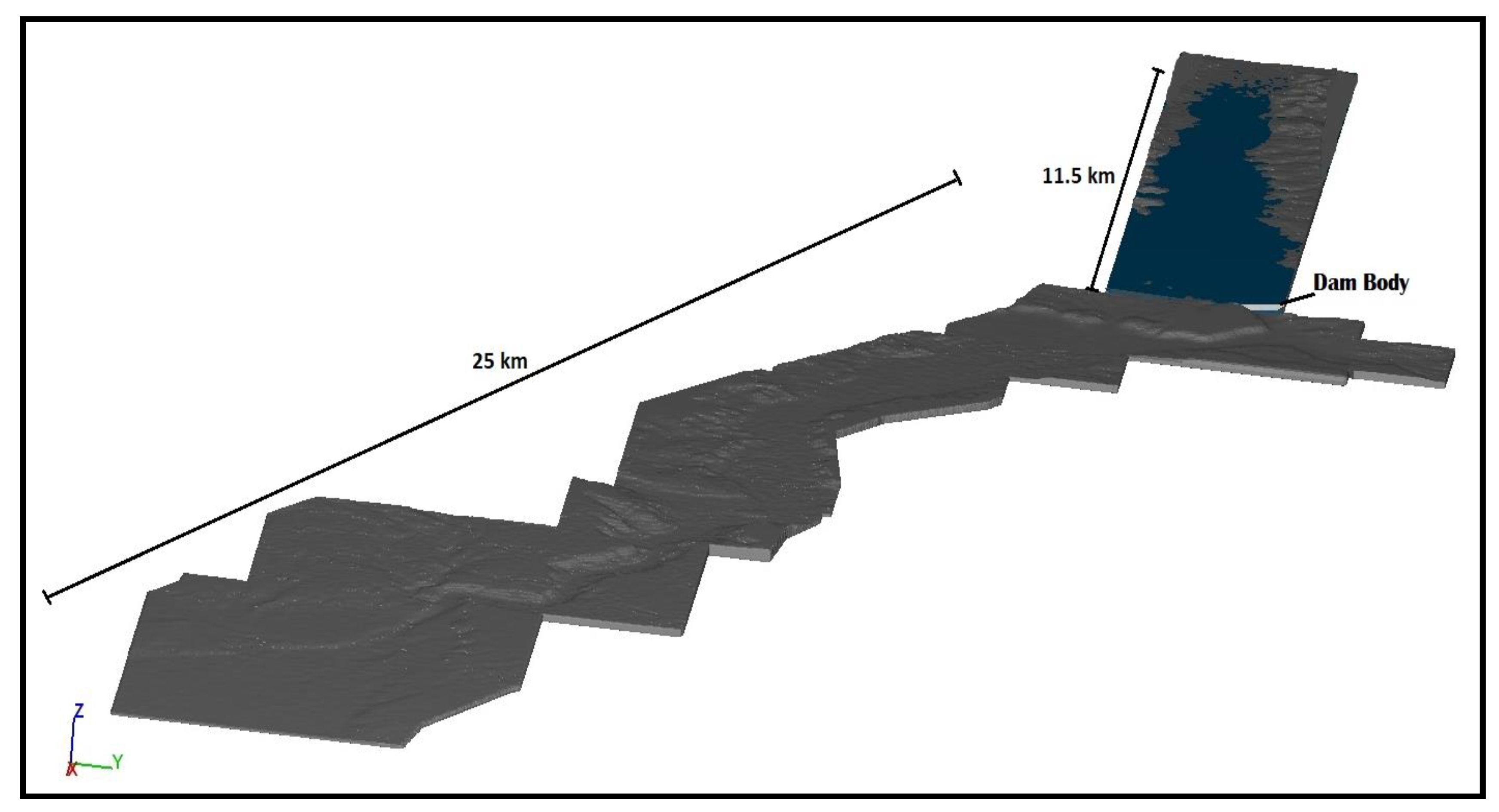
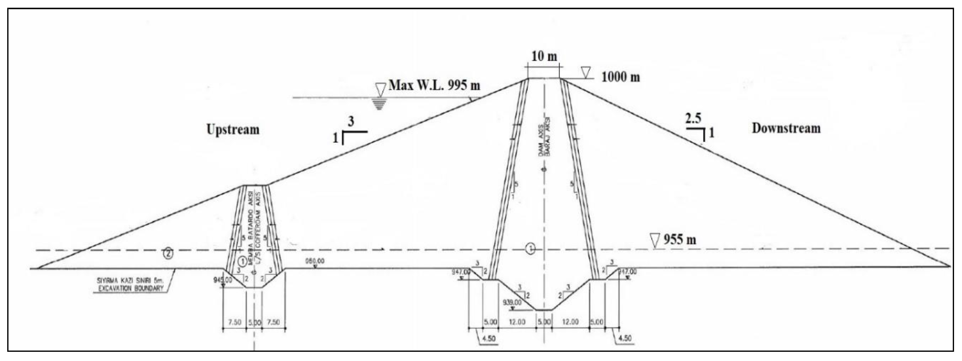
2.1. Study Area and Dam Characteristics
2.2. Geometric Data
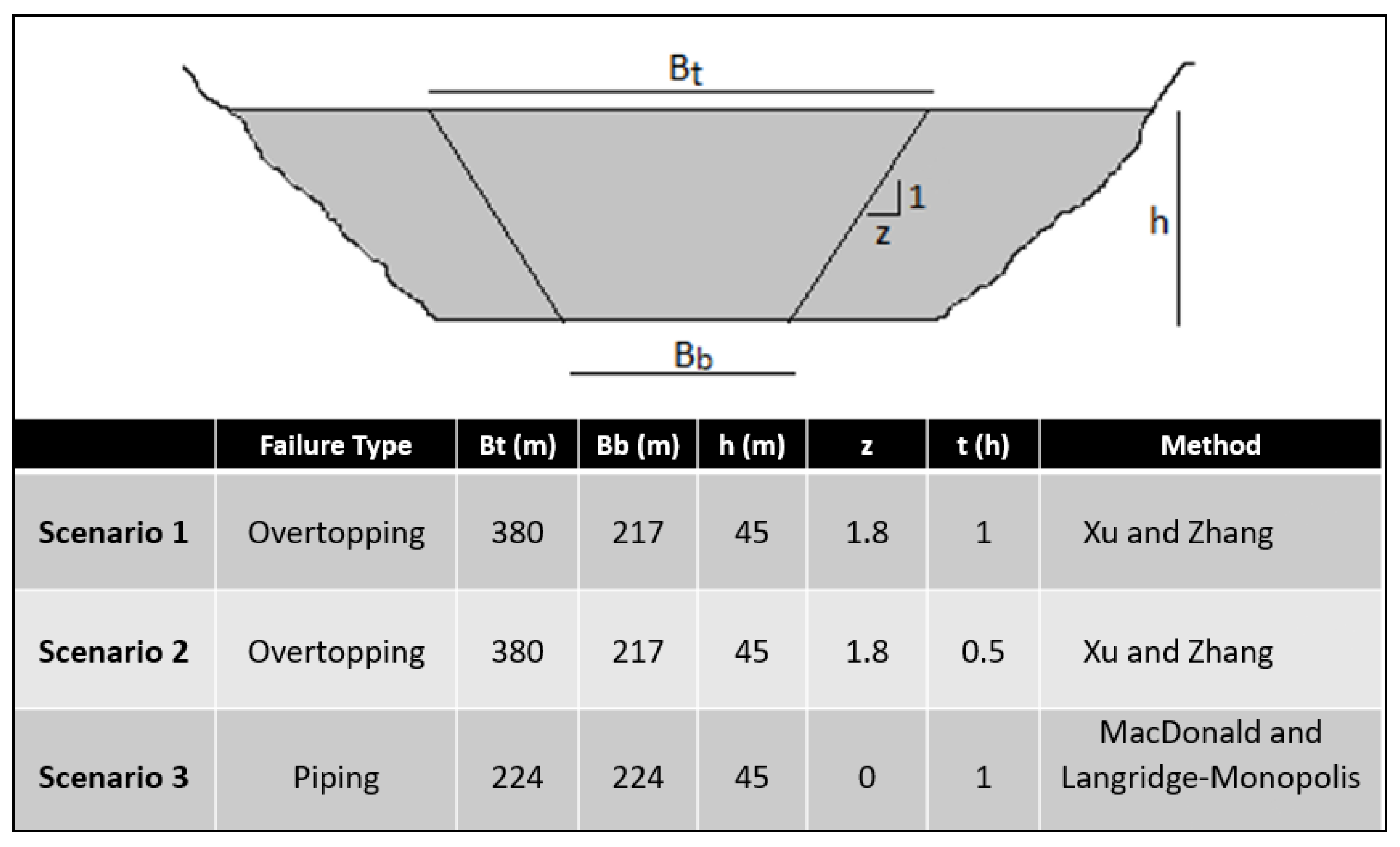
2.3. Estimation of Dam Breach Parameters
2.4. Flow3D Numeric Model
2.4.1. Two-Dimensional Shallow Water Equations
2.4.2. Three-Dimensional Reynolds-Averaged Navier-Stokes Equations
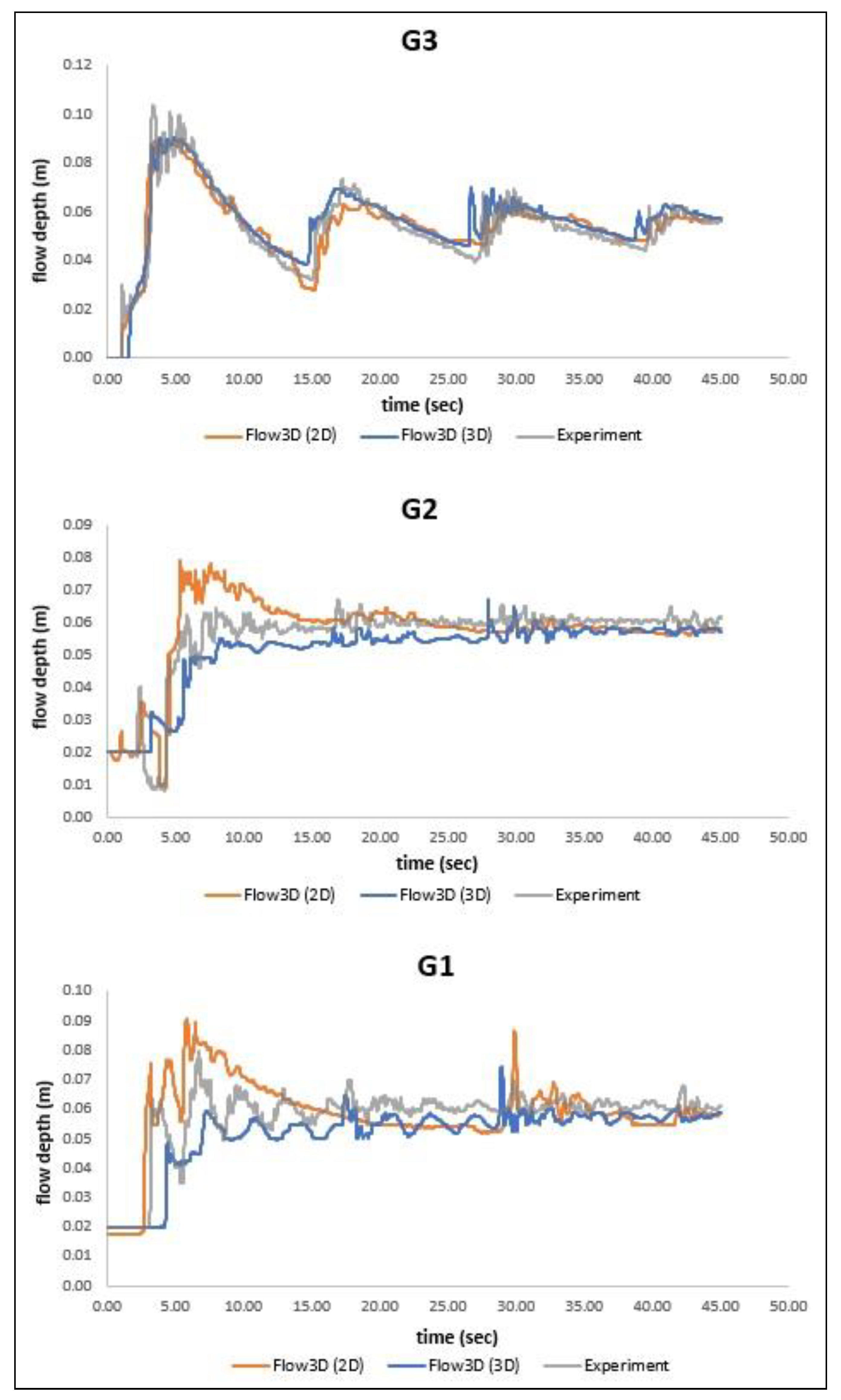
2.5. Model Validation
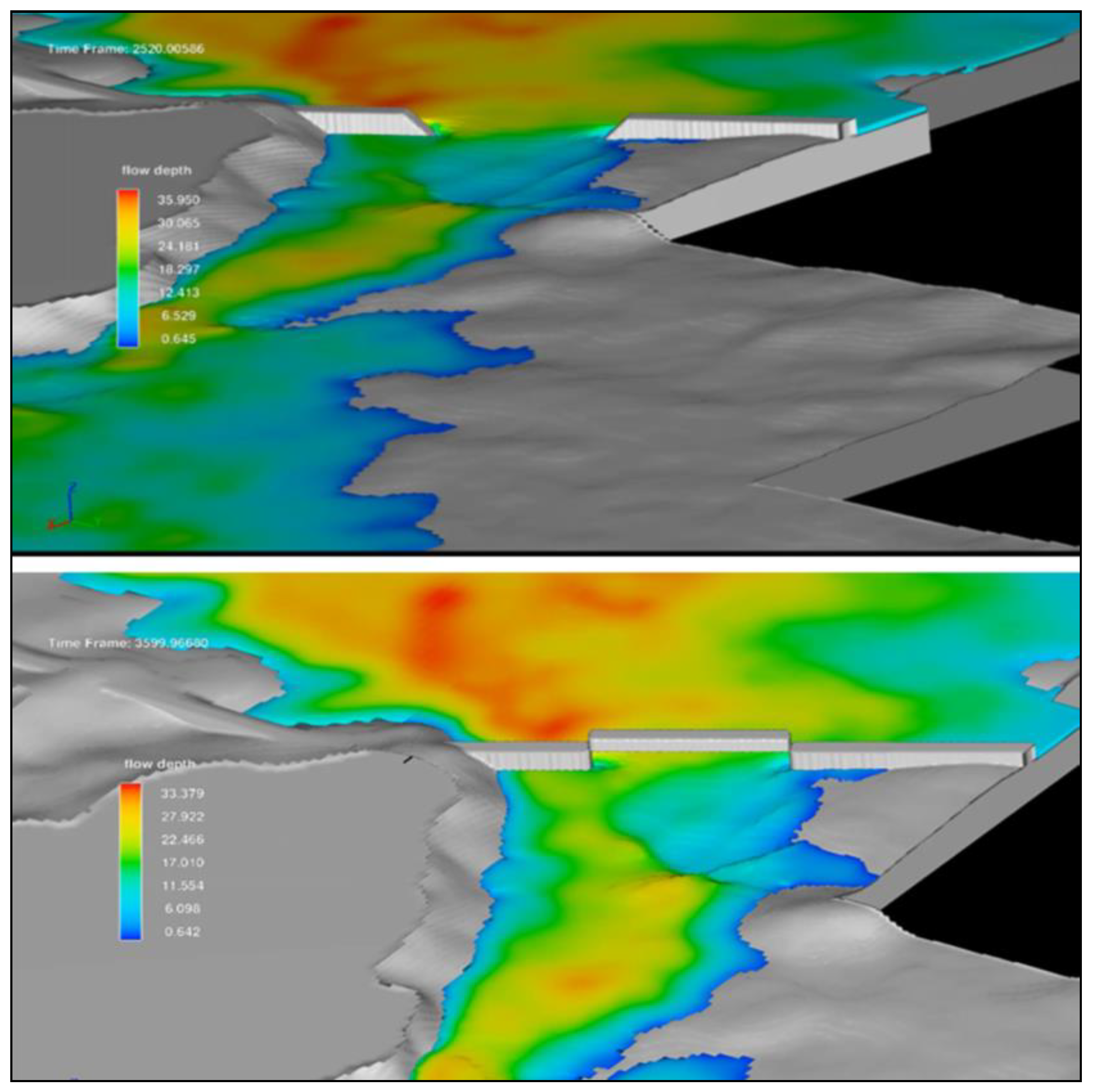
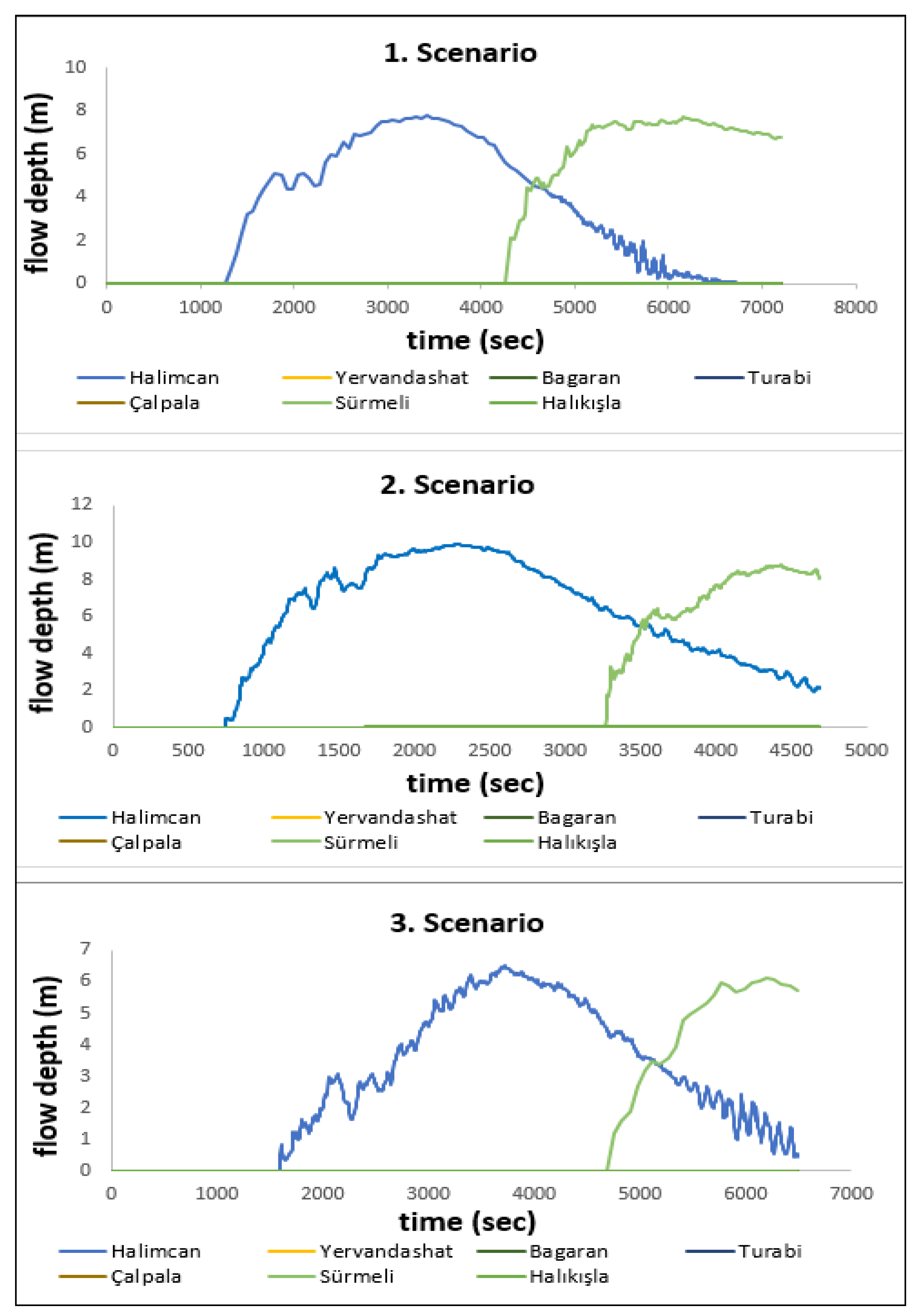
3. Results and Discussion
4. Conclusions
Author Contributions
Funding
Data Availability Statement
Conflicts of Interest
References
- Viseu, T.; de Almeida, A.B. Dam-break risk management and hazard mitigation. State Art Sci. Eng. 2009, 36, 211–239. [Google Scholar]
- Xiong, Y. Dam break analysis using HEC-RAS. J. Water Resour. Prot. 2011, 3, 370–379. [Google Scholar] [CrossRef]
- Le, T.T.H.; Nguyen, V.C. Numerical study of partial dam–break flow with arbitrary dam gate location using VOF method. Appl. Sci. 2022, 12, 3884. [Google Scholar] [CrossRef]
- Adamo, N.; Al-Ansari, N.; Sissakian, V.; Laue, J. Dam safety and overtopping. J. Earth Sci. Geotech. Eng. 2020, 10, 41–78. [Google Scholar]
- Lumbroso, D.; Davison, M.; Body, R.; Petkovšek, G. Modelling the Brumadinho tailings dam failure, the subsequent loss of life and how it could have been reduced. Nat. Hazards Earth Syst. Sci. 2021, 21, 21–37. [Google Scholar] [CrossRef]
- Froehlich, D.C. Embankment Dam breach parameters and their uncertainties. J. Hydraul. Eng. 2008, 134, 1708–1721. [Google Scholar] [CrossRef]
- Najar, M.; Gül, A. Investigating the influence of dam-breach parameters on dam-break connected flood hydrograph. Tech. J. 2022, 33, 12501–12524. [Google Scholar] [CrossRef]
- International Commission onLarge Dams. Dam Failures—Statistical Analysis; Bulletin No. 99; International Commission on Large Dams: Paris, France, 1995. [Google Scholar]
- MacDonald, T.C.; Langridge-Monopolis, J. Breaching characteristics of dam failures. J. Hydraul. Eng. 1984, 110, 567–586. [Google Scholar] [CrossRef]
- Karakaya, K. Numerical Simulation of the Kirazliköprü Dam Failure on the Gökırmak River. Master’s Thesis, Middle East Technical University, Ankara, Turkey, 2005. [Google Scholar]
- Wu, W. Introduction to DLBreach—A Simplified Physically-Based Dam/Levee Breach Model; Technical Report; Clarkson University: Potsdam, NY, USA, 2016. [Google Scholar]
- Ackerman, C.T.; Brunner, G.W. Dam failure analysis using HEC-RAS and HEC-GEORAS. In Proceedings of the 2008 World Environmental and Water Resources Congress, Ahupua’a, Honolulu, HI, USA, 12–16 May 2008. [Google Scholar]
- Li, W.; Zhu, J.; Fu, L.; Zhu, Q.; Xie, Y.; Hu, Y. An augmented representation method of debris flow scenes to improve public perception. Int. J. Geogr. Inf. Sci. 2021, 35, 1521–1544. [Google Scholar] [CrossRef]
- Liu, Z.; Xu, J.; Liu, M.; Yin, Z.; Liu, X.; Yin, L.; Zheng, W. Remote sensing and geostatistics in urban water-resource monitoring: A review. Mar. Freshw. Res. 2023, 74, 747–765. [Google Scholar] [CrossRef]
- Oborie, E.; Rowland, D.R. Flood influence using GIS and remote sensing based morphometric parameters: A case study in Niger delta region. J. Asian Sci. Res. 2023, 13, 1–15. [Google Scholar] [CrossRef]
- Von Thun, J.L.; Gillette, D.R. Guidance on Breach Parameters; Internal Memorandum Rep.; U.S. Department of the Interior, Bureau of Reclamation: Denver, CO, USA, 1990.
- Froehlich, D.C. Embankment dam breach parameters revisited. In Proceedings of the First International Conference on Water Resources Engineering, San Antonio, TX, USA, 14–18 August 1995; American Society of Civil Engineers: New York, NY, USA, 1995; pp. 887–891. [Google Scholar]
- Xu, Y.; Zhang, L.M. Breaching parameters for earth and rockfill dams. J. Geotech. Geoenviron. Eng. 2009, 135, 1957–1970. [Google Scholar] [CrossRef]
- Khoshkonesh, A.; Nsom, B.; Bahmanpouri, F.; Dehrashid, F.A.; Adeli, A. Numerical study of the dynamics and structure of a partial dam-break flow using the VOF method. Water Resour. Manag. 2021, 35, 1513–1528. [Google Scholar] [CrossRef]
- Aureli, F.; Maranzoni, A.; Petaccia, G.; Soares-Frazão, S. Review of experimental investigations of dam-break flows over fixed bottom. Water 2023, 15, 1229. [Google Scholar] [CrossRef]
- Bella, S.W.; Elliot, R.C.; Chaudry, M.H. Experimental results of two dimensional dam-break flows. J. Hydraul. Res. 1992, 30, 225–252. [Google Scholar] [CrossRef]
- Lauber, G.; Hager, W.H. Ritter’s dambreak wave wevisited. In Proceedings of the 27 IAHR Congress, San Francisco, CA, USA, 10–15 August 1997; pp. 258–262. [Google Scholar]
- Ritter, A. Die fortpflanzung de wasserwellen. Z. Ver. Dtsch. Ingenieure 1892, 36, 947–954. (In German) [Google Scholar]
- Soares-Frazão, S. Experiments of dam-break wave over a triangular bottom sill. J. Hydraul. Res. 2007, 45, 19–26. [Google Scholar] [CrossRef]
- Hui, L.; Liu, H.; Guo, L.; Lu, S. Experimental study on the dam-break hydrographs at the gate location. J. Ocean. Univ. China 2017, 16, 697–702. [Google Scholar]
- Stoker, J.J. Water Waves; Interscience Publishers Inc.: Hoboken, NJ, USA, 1957. [Google Scholar]
- Lin, B.; Gong, Z.; Wang, L. Dam-site hydrographs due to sudden release. Sci. Sin. 1980, 23, 1570–1582. [Google Scholar]
- Quecedo, M.; Pastor, M.; Herreros, M.I.; Merodo, J.A.F.; Zhang, Q. Comparison of two mathematical models for solving the dam break problem using the FEM method. Comput. Methods Appl. Mech. Engrg. 2005, 194, 3984–4005. [Google Scholar] [CrossRef]
- Albano, R.; Mancusi, L.; Adamowski, J.; Cantisani, A.; Sole, A. A GIS tool for mapping dam-break flood hazards in Italy. ISPRS Int. J. Geo-Inf. 2019, 8, 250. [Google Scholar] [CrossRef]
- Ríha, J.; Kotaška, S.; Petrula, L. Dam break modeling in a cascade of small earthen dams: Case study of the Cižina River in the Czech Republic. Water 2020, 12, 2309. [Google Scholar] [CrossRef]
- Psomiadis, E.; Tomanis, L.; Kavvadias, A.; Soulis, K.X.; Charizopoulos, N.; Michas, S. Potential dam breach analysis and flood wave risk assessment using HEC-RAS and remote sensing data: A multicriteria approach. Water 2021, 13, 364. [Google Scholar] [CrossRef]
- Bello, D.; Alcayaga, H.; Caamaño, D.; Pizarro, A. Influence of dam breach parameter statistical definition on resulting rupture maximum discharge. Water 2022, 14, 1776. [Google Scholar] [CrossRef]
- Kocaman, S. Experimental and Theoretical İnvestigation of Dam Break Problem. Ph.D. Thesis, Department of Civil Engineering Institute of Natural and Applied Sciences University of Çukurova, Adana, Türkiye, 2007. [Google Scholar]
- Vasquez, J.A. Testing River2D and Flow3D for sudden dam-break flow simulations. In Proceedings of the Conference on Canadian Dam Association, Whistler, BC, Canada, 3–8 October 2009. [Google Scholar]
- Larocque, L.A.; Imran, J.; Chaudhry, M.H. 3D numerical simulation of partial breach dam break flow using the LES and k–Ɛ turbulence models. J. Hydraul. Res. 2013, 51, 145–157. [Google Scholar] [CrossRef]
- Robb, D.M.; Vasquez, J.A. Numerical simulation of dam–break flows using depth-averaged hydrodynamic and three-dimensional CFD models. In Proceedings of the 22nd Canadian Hydrotechnical Conference, Montreal, QC, Canada, 29 April–2 May 2015. [Google Scholar]
- Tahershamsi, A.; Hooshyaripor, F.; Razib, S. Reservoir’s geometry impact of three dimensions on peak discharge of dam-failure flash flood. Sci. Iran. 2017, 25, 1931–1942. [Google Scholar] [CrossRef]
- Franco, A.; Moernaut, J.; Schneider-Muntau, B.; Strasser, M.; Gems, B. The 1958 Lituya Bay tsunami–prevent bathymetry reconstruction and 3D numerical modelling utilising the computational fluid dynamics software Flow-3D. Nat. Hazards Earth Syst. Sci. 2020, 20, 2255–2279. [Google Scholar] [CrossRef]
- Kocaman, S.; Evangelista, S.; Guzel, H.; Dal, K.; Yilmaz, A.; Viccione, G. Experimental and numerical investigation of 3D dam-break wave propagation in an enclosed domain with dry and wet bottom. Appl. Sci. 2021, 11, 5638. [Google Scholar] [CrossRef]
- Republic of Turkey General Directorate of Electricity Works and Studies. Feasibility Report of the Lower Aras Basin Tuzluca Dam and HEPP Project, 2004.
- Bharath, A.; Shivapur, A.V.; Hiremath, C.G.; Maddamsetty, R. Dam break analysis using HEC-RAS and HEC-GeoRAS: A case study of Hidkal dam, Karnataka state, India. Environ. Chall. 2021, 5, 100401. [Google Scholar] [CrossRef]
- Annis, A.; Nardi, F.; Petroselli, A.; Apollonio, C.; Arcangeletti, E.; Tauro, F.; Belli, C.; Bianconi, R.; Grimaldi, S. UAV-DEMs for small-scale flood hazard mapping. Water 2020, 12, 1717. [Google Scholar] [CrossRef]
- Sena, N.C.; Veloso, G.V.; Fernandes-Filho, E.I.; Francelino, M.R.; Schaefer, C.E.G. Analysis of terrain attributes in different spatial resolutions for digital soil mapping application in southeastern Brazil. Geoderma Reg. 2020, 21, e00268. [Google Scholar] [CrossRef]
- Khojeh, S.; Ataie-Ashtiani, B.; Hosseini, S.M. Effect of DEM resolution in flood modeling: A case study of Gorganrood River, Northeastern Iran. Nat. Hazards 2022, 112, 2673–2693. [Google Scholar] [CrossRef]
- Uysal, G.; Tasci, E. Analysis of downstream flood risk in the failure of Batman Dam with two-dimensional hydraulic modeling and satellite data. J. Nat. Hazards Environ. 2023, 9, 39–57. [Google Scholar]
- USBR. Downstream Hazard Classification Guidelines; ACER Tech. Memorandum Rep. No. 11; U.S. Department of the Interior, Bureau of Reclamation: Denver, CO, USA, 1988.
- Yin, Y.P.; Huang, B.L.; Chen, X.T.; Liu, G.N.; Wang, S.C. Numerical analysis of wave generated by the Qianjiangping landslide in three Gorges Reservoir. J. Int. Consort. Landslides 2015, 12, 355–364. [Google Scholar] [CrossRef]
- Flow Science Inc. Flow-3D Version 10.0 User’s Manual; Flow Science Inc.: Santa Fe, New Mexico, 2007. [Google Scholar]
- Tannehill, J.C.; Anderson, D.A.; Pletcher, R.H. Computational Fluid Mechanics and Heat Transfer, 2nd ed.; Taylor & Francis: New York, NY, USA, 1997; p. 792. [Google Scholar]
- Kaheh, M.; Kashefipour, M.A.; Dehghani, A.A. Comparison of k-ɛ and RNG k-ɛ turbulent models for estimation of velocity profiles along the hydraulic jump on corrugated beds. In Proceedings of the 6th International Symposium on Environmental Hydraulics, Athens, Greece, 23–25 June 2010. [Google Scholar]
- Dehdar-behbahani, S.; Parsaie, A. Numerical modeling of flow pattern in dam spillway’s guide wall. Case study: Balaroud dam, Iran. Alex. Eng. J. 2016, 55, 467–473. [Google Scholar] [CrossRef]
- Oliva, J.B.; Valentin, M.G. Comparative Evaluation of Two Different 3D OpenFOAM Modules in a Dam-Break Test. Bachelor’s Thesis, Higher Technical School of Road, Canals Engineering, Barcelona, Spain, 2017. [Google Scholar]
- Ersoy, H.; Karahan, M.; Gelişli, K.; Akgun, A.; Anılan, T.; Sunnetci, M.O.; Yahsi, B.K. Modelling of the landslide-induced impulse waves in the Artvin Dam reservoir by empirical approach and 3D numerical simulation. Eng. Geol. 2019, 249, 112–128. [Google Scholar] [CrossRef]
- Karahan, M.; Ersoy, H.; Akgun, A. A 3D numerical simulation-based methodology for Assessment of landslide-generated impulse waves: A case study of the Tersun Dam reservoir (NE Turkey). J. Int. Consort. Landslides 2020, 17, 2777–2794. [Google Scholar] [CrossRef]
- Aksoy, A.O.; Dogan, M.; Guven, S.O.; Tanır, G.; Guney, M.S. Experimental and numerical investigation of the flood waves due to partial dam break. Iran. J. Sci. Technol. Trans. Civ. Eng. 2022, 46, 4689–4704. [Google Scholar] [CrossRef]
- Shahrim, M.F.; Ros, F.C. Estimation of breach outflow hydrograph using selected regression breach equations. In IOP Conference Series: Earth and Environmental Science; IOP Publishing: Bristol, UK, 2020; p. 476. [Google Scholar]
- Hien, L.T.H.; Nguyen, V.C. Investigate Impact Force of Dam-Break Flow against Structures by Both 2D and 3D Numerical Simulations. Water 2021, 13, 344. [Google Scholar] [CrossRef]
- Zhang, T.; Peng, L.; Feng, P. Evaluation of a 3D unstructured-mesh finite element model for dam-break flood. Comput. Fluids 2018, 160, 64–77. [Google Scholar] [CrossRef]
- Dai, S.; He, Y.; Yang, J.; Ma, Y.; Jin, S.; Liang, C. Numerical study of cascading dam- break characteristics using SWEs and RANS. Water Supply 2020, 20, 348–360. [Google Scholar] [CrossRef]
- Ozmen-Cagatay, H.; Kocaman, S. Dam-break flows during initial stage using SWE and RANS approaches. J. Hydraul. Res. 2010, 48, 603–611. [Google Scholar] [CrossRef]
- DeKay, M.L.; McClelland, G.H. Predicting loss of life in cases of dam failure and flash flood. Risk Anal. 1993, 13, 193–205. [Google Scholar] [CrossRef]
- Graham, W.J. A procedure for estimating loss of life caused by dam failure. Sediment River Hydral. 1999, 6, 1–43. [Google Scholar]
- Jonkman, S.N. Loss of Life Estimation in Flood Risk Assessment. Ph.D. Thesis, Delft University, Delft, The Netherlands, 2007. [Google Scholar]
- Xiaoling, W.; Xuefei, A.; Ruirui, S.; Weiping, G. The comprehensive risk analysis of dam-break consequences based on Numerical Simulation. Appl. Mech. Mater. 2012, 229, 1850–1853. [Google Scholar]
- Sun, R.; Wang, X.; Zhou, Z.; Ao, X.; Sun, X.; Song, M. Study of the comprehensive risk analysis of dam-break flooding based on the numerical simulation of flood routing. Part I: Model development. Nat. Hazards 2014, 73, 1547–1568. [Google Scholar] [CrossRef]
- Sun, R.; Wang, X.; Zhou, Z.; Ao, X.; Sun, X.; Song, M. Study of the comprehensive risk analysis of dam-break flooding based on the numerical simulation of flood routing. Part II: Model application and results. Nat. Hazards 2014, 72, 675–700. [Google Scholar]
- Zhou, K.F. Study on Analysis Method for Loss of Life Due to Dam Breach. Master’s Thesis, Nanjing Hydraulic Research Institute, Nanjing, China, 2006. [Google Scholar]


| Method | Bt (m) | Bave (m) | Bb (m) | Tf (h) | ||||
|---|---|---|---|---|---|---|---|---|
| O | P | O | P | O | P | O | P | |
| MacDonald and Langridge-Monopolis [9] | 341 | 224 | 161 | 224 | 3 | |||
| Bureu of Reclamation [46] | 135 | 1.5 | ||||||
| Von Thun and Gillette [16] | 167 | 1 | ||||||
| Froehlich [17] | 258 | 184 | 2.4 | |||||
| Froehlich [6] | 218 | 156 | 2 | |||||
| Xu and Zhang [18] | 380 | 222 | 287 | 168 | 217 | 87 | 2.4 | 2.3 |
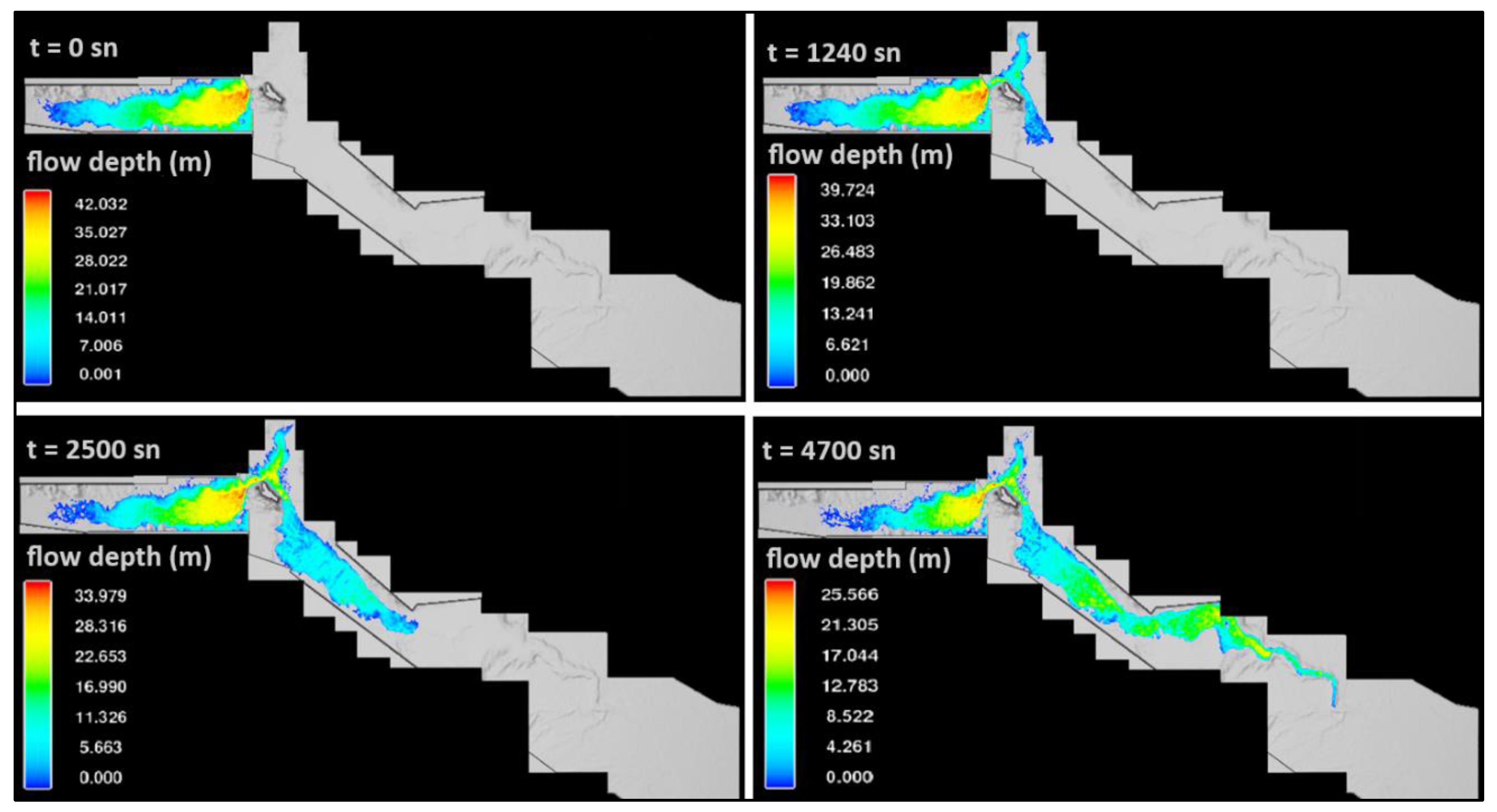
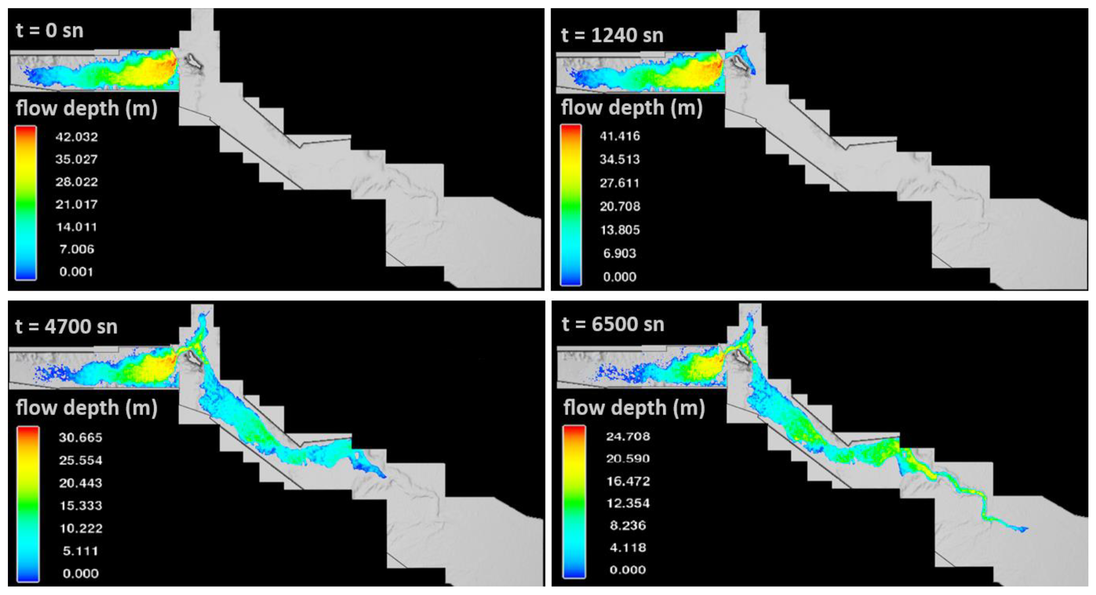
| General | Finish time | 1. Scenario 7200 s |
| 2. Scenario 4700 s | ||
| 3. Scenario 6500 s | ||
| Simulation units | SI | |
| Flow Mode | Incompressible | |
| Physics | Gravity z component | −9.81 m/sn2 |
| Turbulence model | RNG k-ɛ | |
| Fluids | Material | Water at 20 °C |
| Density | 1000 kg/m3 | |
| Meshing and Geometry | Size of cells | 10 m × 10 m; 20 m × 20 m |
| Total number of real cells * | 606,248; 14,823,728 | |
| Mesh type | Cartesian | |
| Boundary conditions ** | Xmin = Wall, Symmetry | |
| Xmax = Symmetry, Outflow | ||
| Ymin * = Wall | ||
| Ymax * = Wall | ||
| Zmin = Wall | ||
| Zmax = Outflow |
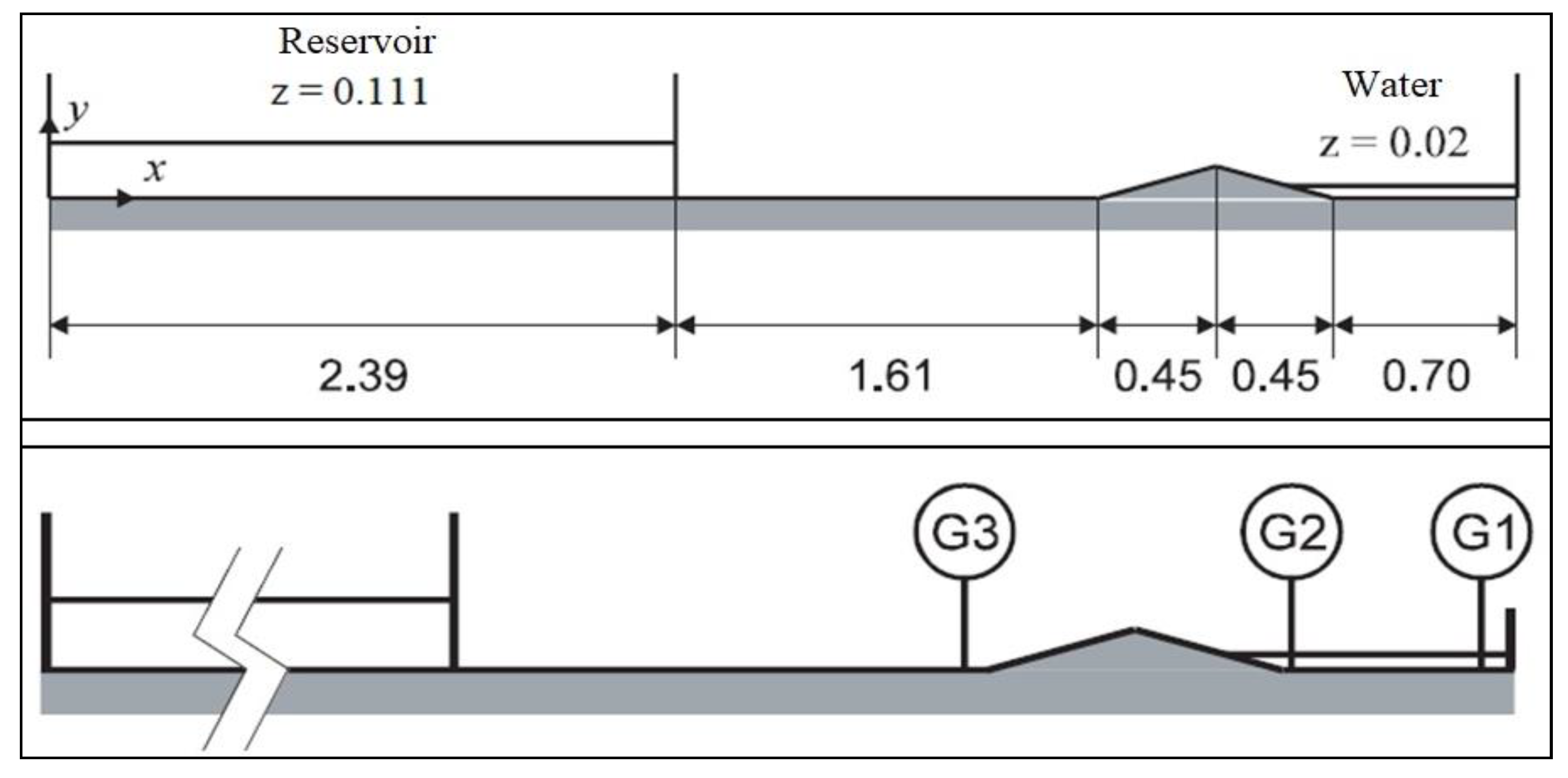
| Level Gauge | x (m) | y (m) |
|---|---|---|
| G1 | 5.575 | 0.25 |
| G2 | 4.925 | 0.25 |
| G3 | 3.935 | 0.25 |
| Probe | RMSE (m) | |
|---|---|---|
| 3D | 2D | |
| G3 | 0.0047 | 0.0048 |
| G2 | 0.0050 | 0.0051 |
| G1 | 0.0048 | 0.0050 |
| si | Population at Risk (Person) | Flood Severity | Warning Time (h) | Local People’s Awareness about Dam Failures |
|---|---|---|---|---|
| 0.80–1.00 | >105 | Extremely high | Wt < 0.25 | Extremely unclear |
| 0.60–0.80 | 104–105 | High | 0.25 < Wt < 0.50 | Unclear |
| 0.40–0.60 | 103–104 | Middle | 0.50 < Wt < 0.75 | Generally clear |
| 0.20–0.40 | 102–103 | Low | 0.75 < Wt < 1.00 | Clear |
| 0.01–0.20 | 1–102 | Extremely low | Wt > 1.00 | Extremely clear |
| Ni | 0.80–1.00 | 0.60–0.80 | 0.40–0.60 | 0.20–0.40 | 0.01–0.20 |
| Young population rate (%) | 0–20 | 20–40 | 40–60 | 60–80 | 80–100 |
| Weather conditions | Heavy storm | Rainstorm | Moderate rain | Sprinkle | Sunny days |
| Time of dam failure | Holiday in the morning | Working day in the morning | Holiday at night | Working days at night | Daytime |
| Distance to the dam (km) | 0–5 | 5–10 | 10–20 | 20–50 | >50 |
| Evacuation and rescue capability | Very unsuccessful | Unsuccessful | General | Successful | Very successful |
| Dam height (m) | >70 | 30–70 | 15–30 | 10–15 | <10 |
| Reservoir capacity | Very Large | Large | Medium | Small | Very Small |
| Downstream slope | Valley | Mountain | Hill | Plain | Beach |
| Building abrasion resistance | Extremely weak | Weak | Middle | Strong | Extremely strong |
| si | Halimcan | Sürmeli | ||||
|---|---|---|---|---|---|---|
| 1. Scenario | 2. Scenario | 3. Scenario | 1. Scenario | 2. Scenario | 3. Scenario | |
| s1 | 0.10 | 0.10 | 0.10 | 0.30 | 0.30 | 0.30 |
| s2 | 0.60 | 0.80 | 0.50 | 0.60 | 0.80 | 0.50 |
| s3 | 0.70 | 0.90 | 0.65 | 0.10 | 0.20 | 0.05 |
| s4 | 0.70 | 0.70 | 0.70 | 0.70 | 0.70 | 0.70 |
| ni | Halimcan | Sürmeli |
|---|---|---|
| 1., 2. and 3. Scenarios | 1., 2. and 3. Scenarios | |
| n1 | 0.50 | 0.50 |
| n2 | 0.40 | 0.40 |
| n3 | 0.50 | 0.50 |
| n4 | 0.90 | 0.50 |
| n5 | 0.40 | 0.40 |
| n6 | 0.65 | 0.65 |
| n7 | 0.60 | 0.60 |
| n8 | 0.80 | 0.90 |
| n9 | 0.80 | 0.80 |
| Halimcan LOL (Person) | Sürmeli LOL (Person) | Total LOL (Person) | |
|---|---|---|---|
| 1. Scenario | 22 | 179 | 201 |
| 2. Scenario | 25 | 202 | 227 |
| 3. Scenario | 21 | 170 | 191 |
Disclaimer/Publisher’s Note: The statements, opinions and data contained in all publications are solely those of the individual author(s) and contributor(s) and not of MDPI and/or the editor(s). MDPI and/or the editor(s) disclaim responsibility for any injury to people or property resulting from any ideas, methods, instructions or products referred to in the content. |
© 2023 by the authors. Licensee MDPI, Basel, Switzerland. This article is an open access article distributed under the terms and conditions of the Creative Commons Attribution (CC BY) license (https://creativecommons.org/licenses/by/4.0/).
Share and Cite
Akgun, C.; Nas, S.S.; Uslu, A. 2D and 3D Numerical Simulation of Dam-Break Flooding: A Case Study of the Tuzluca Dam, Turkey. Water 2023, 15, 3622. https://doi.org/10.3390/w15203622
Akgun C, Nas SS, Uslu A. 2D and 3D Numerical Simulation of Dam-Break Flooding: A Case Study of the Tuzluca Dam, Turkey. Water. 2023; 15(20):3622. https://doi.org/10.3390/w15203622
Chicago/Turabian StyleAkgun, Cagri, Salim Serkan Nas, and Akin Uslu. 2023. "2D and 3D Numerical Simulation of Dam-Break Flooding: A Case Study of the Tuzluca Dam, Turkey" Water 15, no. 20: 3622. https://doi.org/10.3390/w15203622
APA StyleAkgun, C., Nas, S. S., & Uslu, A. (2023). 2D and 3D Numerical Simulation of Dam-Break Flooding: A Case Study of the Tuzluca Dam, Turkey. Water, 15(20), 3622. https://doi.org/10.3390/w15203622