Algae in a Drinking Water Reservoir: Development of an Air–Water–Algal Growth Model (AWAM) for Long-Term Prediction

Abstract

The condition of the water in drinking water source environments is critical for public health. However, in recent years, the rapid growth of algae has become a significant threat to the safety of the drinking water supply. This study investigated the temporal trends and spatial differences in algae in the Nanwan Reservoir during 2022. Regression analysis using the least-squares method demonstrated that water temperature and initial biomass concentration were critical parameters that influenced the rate of algal growth. An air–water–algal growth model (AWAM) for algal growth prediction was developed using a 30-day forecast of air temperature, an air-to-water temperature extrapolating equation, a water temperature–algal growth relationship, and only four monthly measurements of algal concentration. The results demonstrated that the model accurately predicted algal growth in the next 30 days, with an R² of 0.738, which aligned with the monitored results. Compared to the upstream Wudaohe River inflow point, algal growth in the drinking water intake area near the downstream dam was delayed by at least 30 days. By using the upstream inflow area as a reference point, the prediction period was extended to provide a 60-day early warning. The extended prediction period and the reduced need for monitoring data make the model more convenient for guiding the prevention and control of algal blooms in drinking water reservoirs.

1. Introduction

As primary producers, Cyanobacteria and algae play a crucial role in aquatic ecosystems [1]. However, ongoing global warming and anthropogenic activities have led to their excessive growth and subsequent algal blooms, resulting in environmental problems such as ecosystem disruption and threats to the drinking water supply [2,3]. Unfortunately, global reservoirs and lakes are increasingly susceptible to persistent and widespread algal blooms [4]. The water quality of a reservoir is directly linked to public water safety. Predicting algal growth is crucial for the development of effective strategies to control algal blooms.

The algal growth prediction model is designed to quantitatively forecast the future growth pattern of algae using the laws governing algal growth. These models can proactively assess the likelihood and extent of algal blooms, providing valuable data to guide the development of measures for preventing and controlling algal blooms and ensuring the safety of the drinking water supply [5,6]. Research on algal bloom prediction technology started in the late 20th century and has rapidly progressed in recent years.

Over the past two decades, prediction accuracy for algal blooms has reached a high level using training models that rely on historical data [7]. Intelligent algorithm-based algal bloom prediction models, including simulation models and artificial neural networks [8,9], are widely utilized among the current prediction methods for algal blooms in lakes and reservoirs [10]. These models, based on mathematical algorithms and artificial intelligence, establish a nonlinear relationship between data by fitting historical data [11,12]. Despite their high prediction accuracy, these models provide limited insight into the growth characteristics of algae, hindering the exploration of the underlying mechanisms of algal proliferation. Furthermore, they rely on a substantial amount of historical data for initial learning, which adds complexity to the prediction process.

Currently, most efforts in algal bloom prediction focus on short-term forecasts within a two-week timeframe, with limited reports on long-term predictions [11]. Algal bloom occurrences in large lakes and reservoirs often exhibit spatial variations, with algal growth typically emerging earlier in the shallow waters of river inflows compared to intake areas near downstream dams [13,14]. By identifying the key factors influencing algal growth rates in upstream river flows and downstream intake areas, as well as determining the time differences in rapid growth, it becomes possible to provide early warnings for algal growth in an intake area.

The occurrence of algal blooms is affected by various environmental factors, mainly nutritional, meteorological, hydrological, physical, and chemical indicators of water bodies as well as biological factors [15,16,17,18]. Constructing a model encompassing all factors related to blooms is impractical, since the variables that most accurately explain their occurrence do not consistently predict it [19]. In mesotrophic lakes, changes in nutrients are not the main factors that influence algal blooms [20]; for example, global changes, including increased temperatures, altered precipitation, and reduced acidification, provide suitable environmental conditions for algal blooms [21]. It is reported that water temperature is a critical parameter affecting the occurrence of blooms [22]. On the other hand, water temperature may prove more effective in predicting bloom dynamics [23,24].

This study establishes an air–water–algal growth model (AWAM) based on key parameters for a typical drinking water source, the Nanwan Reservoir. The objectives of this study are (1) to develop a long-term prediction algal growth model by incorporating forecasted air temperatures and indicators of algal growth in the upstream estuary and (2) to simplify input data requirements using an algal-growth-regulated logistic model. By addressing limitations, such as data scarcity and short prediction horizons encountered in existing models, the developed AWAM can offer valuable insights for developing effective measures to control algae in drinking water reservoirs.

2. Material and Methods

2.1. Nanwan Reservoir and Sampling Points

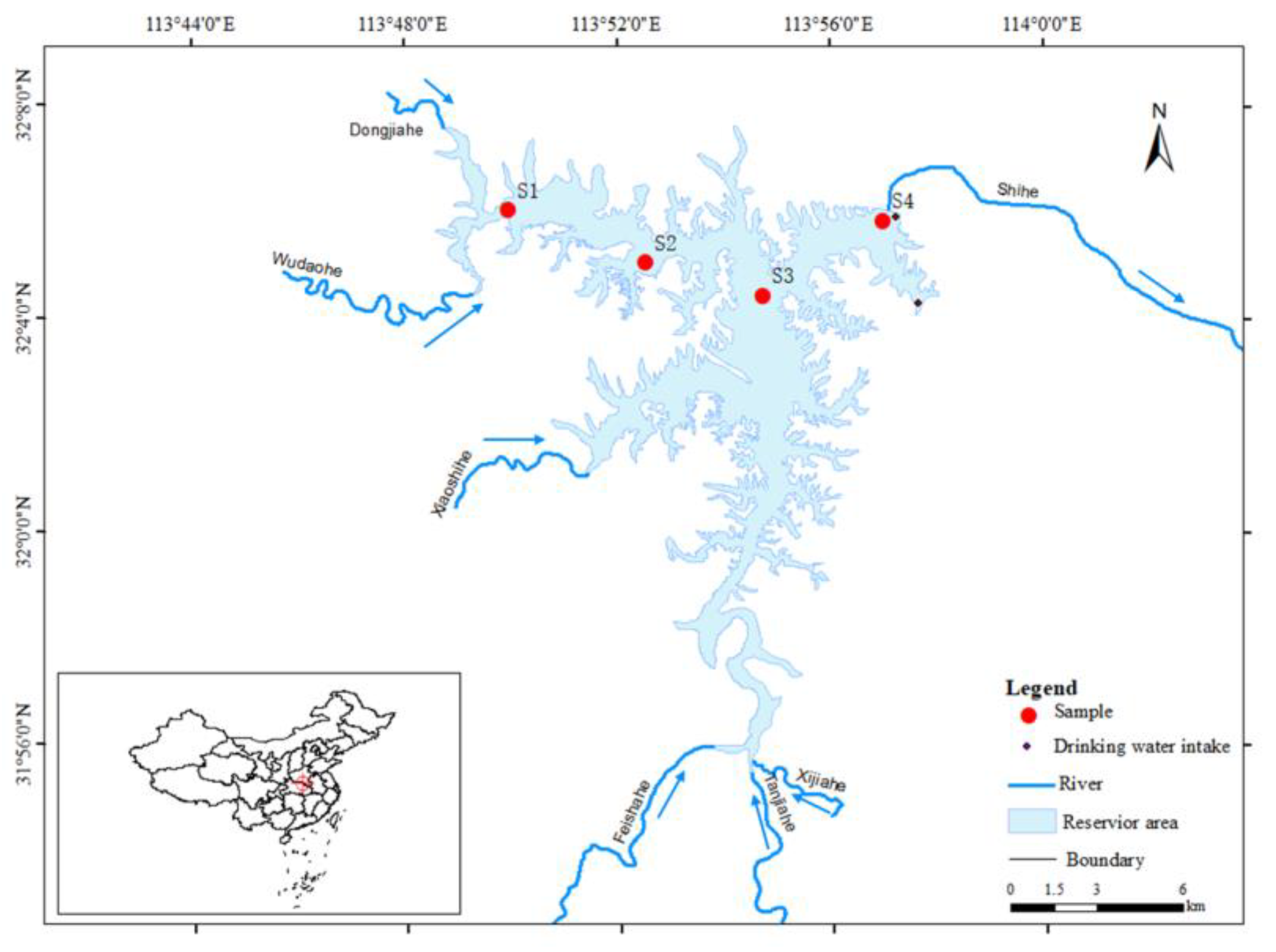
The Nanwan Reservoir (31.95° N–32.15° N, 113.87° E–114.02° E), located on the Shihe River, a tributary of Huai River, is one of the first large-scale projects constructed and serves as a key project for flood control and water management in the Huai River Basin. The Nanwan Reservoir has a surface area of 70 km², a basin area of 1100 km², a water volume of 1.63 billion cubic meters, and an average water depth of 17 m when the water level is 103 m (relative to sea level). The water sources of the Nanwan Reservoir mainly come from nearby river networks, including the Wudaohe River, Dongjiahe River, Tanjiahe River, Xijiahe River, Feishahe River, and Xiaoshihe River (Figure 1). However, there have been occurrences of algal blooms at the inflow area in the reservoir in recent years, with Microcystis spp. being the dominant species during these periods [25].

Our study started from the Wudaohe River inflow point into the midpoint of the Nanwan Reservoir and extended to the dam front area. Within the study area, four sampling points were established (Figure 1) and named S1–S4 (S1: Wudaohe River Inflow Point; S2: Upper Sampling Point in Nanwan Reservoir; S3: Mid Sampling Point in Nanwan Reservoir; and S4: City Drinking Water Intake Point near the Dam).

2.2. Meteorological and Water Quality Analysis

The daily temperature data were obtained from the official weather information of Xinyang City, Henan Province, China, provided by the China Meteorological Administration (http://cdc.cma.gov.cn/, accessed on 17 August 2022). Historical maximum temperatures were included to fit the air–water temperature model, and future weather forecasts were utilized for AWAM prediction. Daily historical water temperature data to fit the air–water temperature model were obtained from the National Surface Water Quality Automatic Monitoring Platform Data Release System (https://www.mee.gov.cn/, accessed on 31 December 2021), which publishes the temperature data for the Nanwan Reservoir National Control Section.

Water measurements were taken at the four sampling points (S1–S4) for water temperature (WT), pH, turbidity (Tur), and dissolved oxygen (DO) using a portable multi-parameter water quality sensor (Yushan, Y4000, Suzhou, China).

Water sample collection was carried out every 20 days. Quantitative samples of phytoplankton were collected using an acrylic water sampler; 1 L water samples were taken at depths of 0.5 m, 2.5 m, and 5.5 m, respectively. After mixing, a portion of the samples was transferred into a 1 L and a 0.5 L bottle. The 1 L samples were spiked with 10 mL Lugol’s solution immediately on the boat. The 0.5 L bottles were brought back to the laboratory under refrigerated and dark conditions for algal biomass measurement.

The supernatant was removed, and the sediment was collected after 24 h of settlement. The dominant algal species was Microcystis spp., in the forms of colonies or aggregates, and 24 h settlement was long enough for their concentration. In the pre-experiment, at least 10 supernatant samples were checked under a microscope using a 0.1 mL plankton counting chamber, and no cells or colonies were found. Samples with Lugol’s solution that were allowed to settle for 24 h were then concentrated at 40 times and thoroughly mixed, before 0.1 mL was taken for counting in a plankton counting chamber and identified using a light microscope (Olympus, CX 23, Olympus Corporation, Tokyo, Japan) following the methods described in “Freshwater Algae of China: Systematics, Classification, and Ecology” [26] and “Water and Wastewater Monitoring and Analysis Methods (4th Edition)” [27]. Each Lugol-fixed sample was counted at least twice, and the average value was reported.

Algal biomass was determined using the dry weight method (DW) [28,29]. Firstly, glass microfiber filters (Whatman, GF/C 1825-055, GE Healthcare Life Sciences, Little Chalfont, UK) were weighed (W₁, mg) after drying at 105 °C for 6 h. Then, a 0.5 L sample was filtered onto a drying glass microfiber filter via a vacuum pump and dried at 105 °C for 24 h. The dried algal biomass and filter were then weighed (W₂, mg) using an analytical balance with a readability of 0.01 mg (METTLER, MA205DU, METTLER TOLEDO, Greifensee, Switzerland). The calculation equation is as follows:

$$\mathrm{D}\mathrm{W},\mathrm{m}\mathrm{g}/\mathrm{L}=\frac{\left({\mathrm{W}}_2-{\mathrm{W}}_1\right)\times 1000}{\mathrm{s}\mathrm{a}\mathrm{m}\mathrm{p}\mathrm{l}\mathrm{e} \mathrm{v}\mathrm{o}\mathrm{l}\mathrm{u}\mathrm{m}\mathrm{e},\mathrm{m}\mathrm{L}}$$

(1)

Based on the above description, the main experimental processes are shown in Figure 2.

The dry weight of the algae obtained from the first sampling was defined as the initial biomass concentration. The daily growth rate of algal biomass was used to evaluate the involution of an algal bloom, and the unit was mg/L/d. The daily growth rate was calculated using the measured dry weight method (DW); the calculation equation is as follows:

$$\mathrm{G}\mathrm{r}\mathrm{o}\mathrm{w}\mathrm{t}\mathrm{h} \mathrm{R}\mathrm{a}\mathrm{t}\mathrm{e},\frac{\mathrm{m}\mathrm{g}}{\mathrm{L}}/\mathrm{d}=\frac{{\mathrm{D}\mathrm{W}}_{\mathrm{t}2}-{\mathrm{D}\mathrm{W}}_{\mathrm{t}1}}{\mathrm{t}2-\mathrm{t}1}$$

(2)

2.3. Model Development

2.3.1. Calculation of Surface Water Temperature

The calculation method for surface water temperature in the reservoir is based on the relationship model between daily maximum water temperature and air temperature developed by Daniel Caissie [30,31]. In this study, earlier data from November 2020 to November 2021, covering a total of 13 months, were used to fit the model parameters and obtain the key parameter values applicable to the Nanwan Reservoir. The calculation equation is as follows:

$${WT}_t=5.83+\frac{22.47}{1+EXP [0.22\times (19.8-{AT}_t\left)\right]}$$

(3)

where AT_t is the air temperature at time t, and WT_t is the surface water temperature at time t. The predictive accuracy of the model reaches R² = 0.74.

2.3.2. Algal Growth Rate Calculation

The least-squares method is a classical approach used for regression fitting. It is used to minimize the sum of squared errors to find the optimal fitting parameters for a function. This method is capable of accurately and comprehensively handling raw observed data and is not limited by the number of sampling points. After taking the logarithm of the selected independent variables, a regression analysis was performed using the least-squares method, comparing it with the algal growth rates obtained from previous investigations. This analysis resulted in the calculation equation for the growth rate coefficient as follows:

$$k=\alpha \ln \left(D_1\right)+\beta \ln \left(D_2\right)+\cdots +\xi \ln \left(D_n\right)+\gamma$$

(4)

where k is the growth rate parameter; α, β, ξ, and γ are variable parameters obtained from the least-squares regression; D₁, D₂, …, D_n are the environmental variables; and γ is a constant.

By conducting correlation analysis, this study aims to explore the correlation between algal biomass and environmental factors and select the environmental factor D_i with the highest correlation from the analysis results as one of the input variables for the model.

Previous research has indicated that the initial biomass concentration of algae significantly affects its growth in the subsequent stages. Therefore, this study selected the initial biomass concentration as one of the input variables for the model. The final equation for calculating the growth coefficient is as follows:

$$k=\alpha \ln \left(C_0\right)+\beta \ln \left(D_i\right)+\gamma$$

(5)

where C₀ is the initial biomass concentration, D_i is another environmental variable, α and β are the coefficients for the initial biomass concentration and environmental factor, and γ is a constant.

2.3.3. Model of Algal Growth

The logistic model is a well-known growth theory curve characterized by three phases: slow growth in the early stage; rapid growth in the middle stage; and then a transition to slow growth again, forming an “S” shape [32]. The equation represents ecological information about algal growth, and the quantitative parameters obtained through specific calculations provide insight into the algal growth pattern. Algal community structure varies among different lakes and reservoirs and is influenced by hydrological features and characteristics. Additionally, algal biomass is affected by vertical gradient differences in water temperature. Thus, adjusting the obtained biomass with a correction factor, denoted as F, is necessary. This provides the final predicted algal biomass calculation equation as follows:

$$C_t=\frac{A}{1+EXP(B-kt)}\times F$$

(6)

where A is the highest algal concentration in the prediction area, which can be obtained through in situ growth rate tests or historical data; t is the number of days of algal growth; B is the time when the growth curve begins to exhibit rapid growth; k is the growth rate coefficient of algae under certain environmental conditions; and F is the correction factor.

In this Nanwan Reservoir case study, considering the variation in water depth from the Wudaohe River inflow points to the dam, the correction factor is calculated using the following formula:

$$F=\frac{H_{min}}{H_i}$$

(7)

where H_min is the depth in the upstream sampling point of the reservoir (S1), and H_i is the depth at each sampling point. Finally, the corresponding values of A, B, and F for the four regions are different (

Table 1. The constants for each sample.

Sample	A	B	F
S1	7.60	3.10	1.0
S2	5.20	2.80	0.8
S3	6.10	2.20	0.5
S4	5.25	1.50	0.5

).

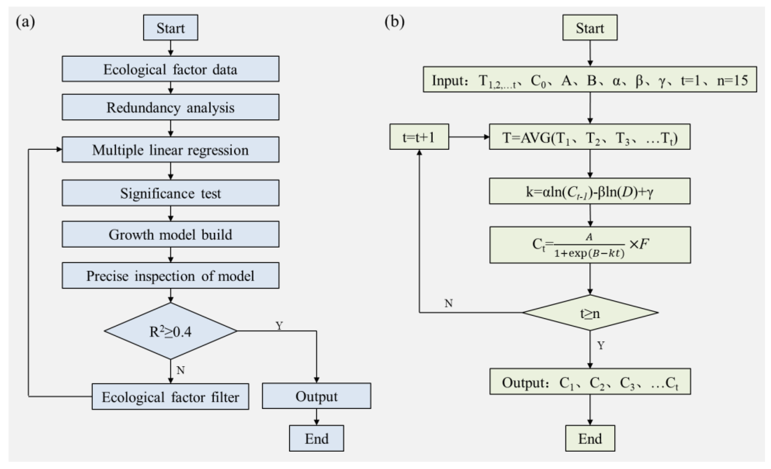
Based on the above description, the model development process mainly involved five steps: acquiring initial data; screening environmental factors; establishing regression equations; constructing prediction models; and testing accuracy, the key to which was to combine the growth rate coefficient equation with the logistic model (Figure 3).

2.4. Statistical Analysis

Raw data processing and analyses were performed using Excel 2019. Basic graphs were plotted using Origin Pro 2019. Redundancy analysis was conducted using Canoco 5.0 to analyze the correlation between algal biomass and environmental factors. Significance testing of the data was carried out using IBM SPSS 21 software. Algal biomass and environmental factor data were transformed using the natural logarithm (ln(D_i)), and regression analysis of algal biomass and environmental factors were performed using the least-squares method.

3. Results and Discussion

3.1. Spatial and Temporal Dynamics of Algae

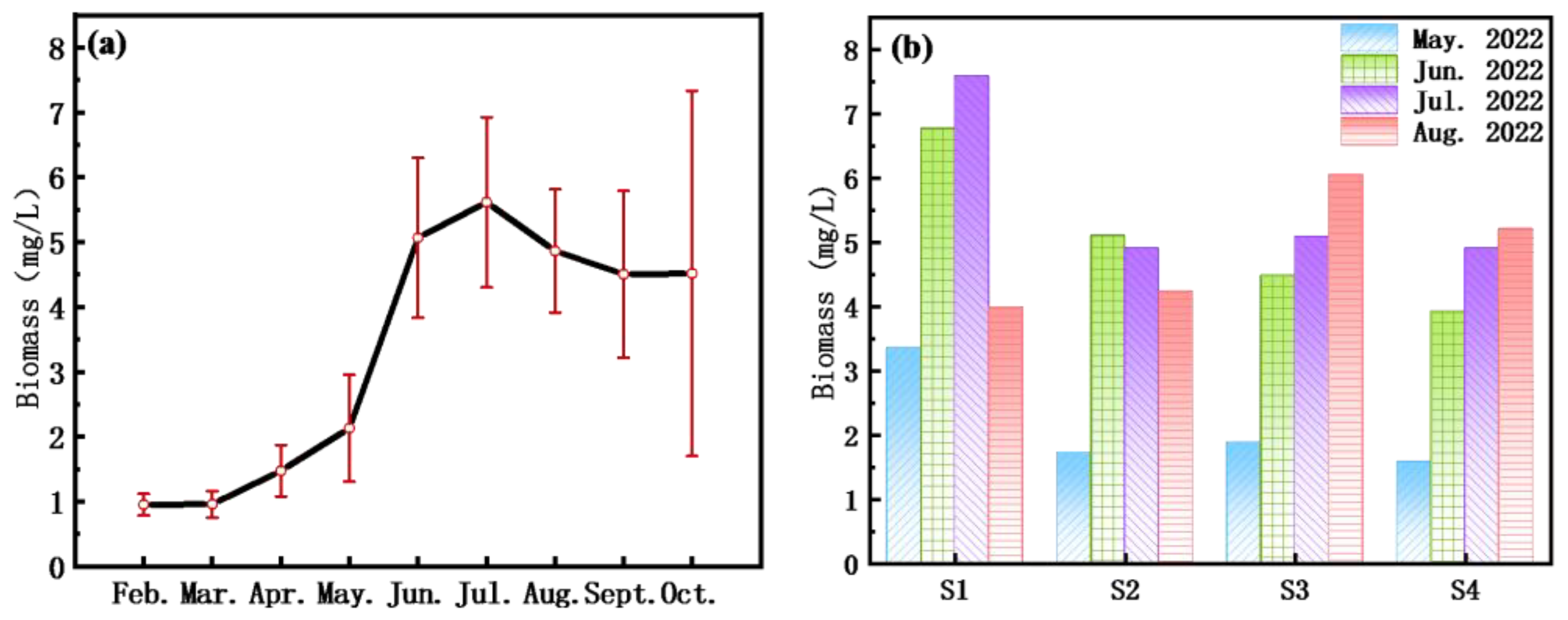
The biomass of algae varied between 0.95 and 5.62 mg/L, exhibiting an overall increasing trend from February to July (Figure 4a) followed by a gradual decline from July to October. Observing the spatial patterns in the Nanwan Reservoir, the Wudaohe River inflow area reached its maximum biomass in July before declining, while the central region and the area in front of the dam showed a consistent increasing trend throughout the study period (Figure 4b). In August, the biomass in these areas was higher than that in the Wudaohe River inflow area and the upstream areas. After entering the autumn season, a decrease in temperature and an increase in rainfall affected the accumulation of algae, leading to an overall reduction in algal biomass. This influence was particularly noticeable in the shallow regions near the reservoir entrance.

A total of 72 species spanning 7 phyla of algae were collected during the study period in the Nanwan Reservoir. Cyanobacteria, Chlorophyta, and Bacillariophyta accounted for a substantial portion, ranging from 75% to 89% of the total composition, while Cryptophyta, Dinophyta, and Euglenophyta constituted a smaller proportion, varying between 11% and 25%. In the months of February and March, Chlorophyta and Bacillariophyta were the dominant groups in the algal community of the Nanwan Reservoir. However, starting from April, the proportion of Cyanobacteria gradually increased, exceeding 80% in July, before experiencing a subsequent decline. Chlorophyta, on the other hand, fluctuated within a narrow range of 8% to 13%. Although Bacillariophyta exhibited higher proportions in February and March, they did not maintain dominance from June to August. The temporal change of algal community structure is presented in the Supplementary Materials (Figure S1).

In a previously conducted survey, a comprehensive identification of algal species in the Nanwan Reservoir resulted in the recognition of a total of 148 species belonging to 7 phyla, with Cyanobacteria constituting less than 70% of the identified species [25]. However, the results of our study suggested a decline in algal species diversity in the Nanwan Reservoir, while the quantity of Cyanobacteria increased. As a result, the period between June and September exhibited relatively high levels of Cyanobacteria, potentially elevating the risk of harmful algal blooms in the Nanwan Reservoir.

3.2. Meteorological and Water Quality Conditions

Our results showed changes in light intensity, water temperature, precipitation, and water level in the Nanwan Reservoir from June 2021 to August 2022 (Figure 5). The water level fluctuated within the range of 98.8 to 99.3 m, without significant temporal patterns attributable to water diversion influences. In terms of light intensity, a distinct seasonal trend was observed, influenced by solar radiation, with values surpassing 1200 μmol/m²/s during the period from June to September. The peak light intensity of 2389 μmol/m²/s occurred annually in June. Throughout the investigation period, the water temperature in the Nanwan Reservoir varied between 6.5 and 32.7 °C. The temperature experienced a gradual rise from 25 °C in May and consistently remained around 30 °C until August. It is worth mentioning that during this period, the reservoir demonstrated higher concentrations of algal biomass. Previous studies have emphasized that temperatures exceeding 27 °C are conducive to the proliferation of cyanobacteria, making water temperature a crucial influencing factor contributing to algal bloom in the Nanwan Reservoir. The highest amount of precipitation was observed in July of each year, with 141.4 mm of rainfall in July 2021, accounting for 24.1% of the total annual precipitation, and 86.2 mm in July 2022, accounting for 28.8% of the total annual precipitation. Due to its shallow water depths, the Wudaohe River inflow area is more vulnerable to the effects of inflowing streams. Therefore, an increase in rainfall could be considered as one factor contributing to the decrease in algal biomass in August at S1.

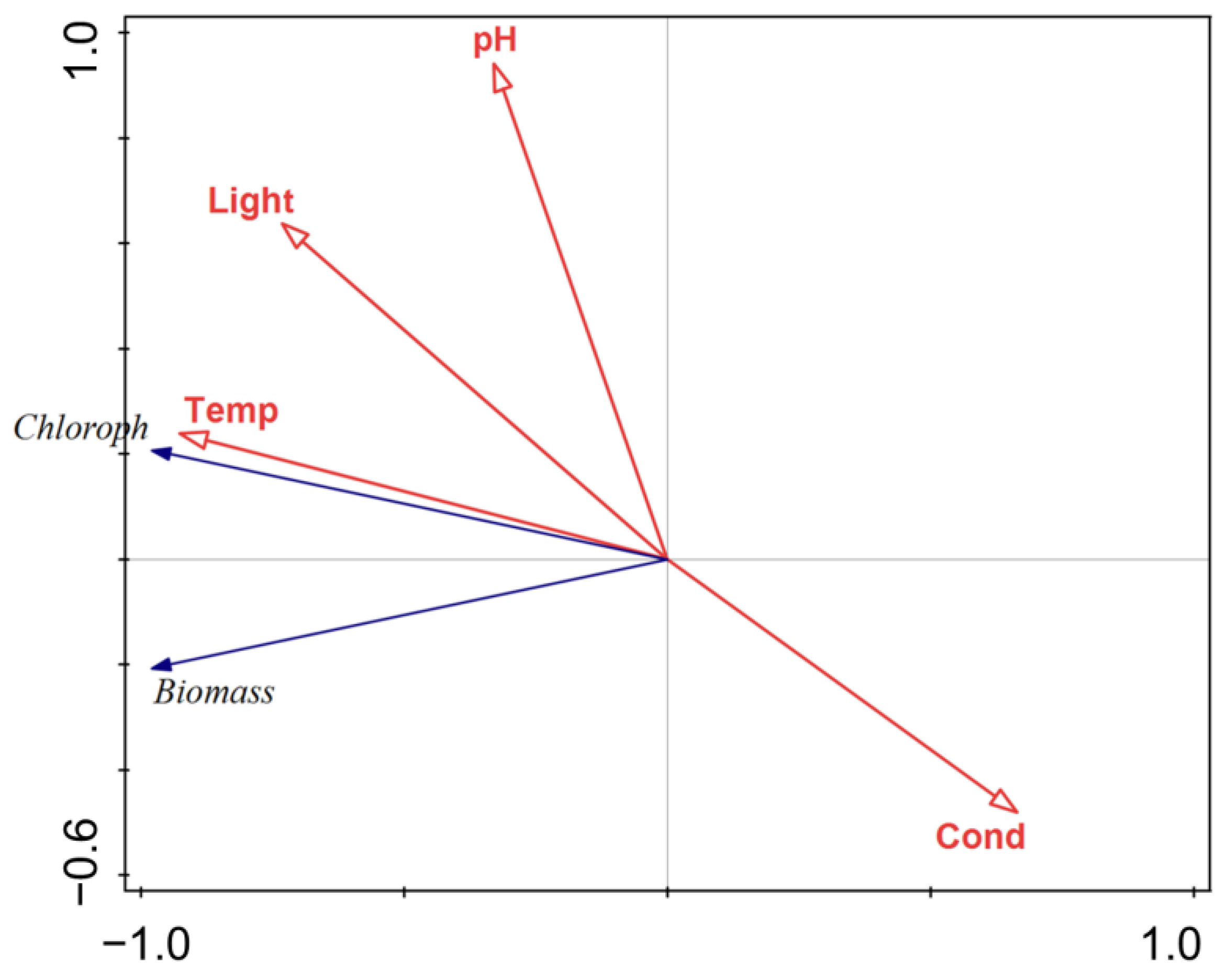
According to recent research, current global climate change has shifted the limiting factor for algal growth from nutrient conditions to water temperature, which plays a crucial role in algal proliferation [33,34]. To examine the association between algal biomass and environmental factors in the Nanwan Reservoir, a redundancy analysis (RDA) was employed. This analysis encompassed algal biomass along with environmental factors such as water temperature, light intensity, pH, and conductivity (Figure 6). The result revealed a positive correlation between algal biomass and pH, light intensity, and water temperature. Among these factors, water temperature demonstrated the highest sensitivity and significantly influenced the variation in algal biomass.

The spatial and temporal distribution patterns of algae are closely intertwined with environmental factors, especially the characteristics of water temperature, and the influence of these environmental factors on algae differs depending on the time frame considered. In this study, the variation in algal biomass within the Nanwan Reservoir displayed distinct seasonal attributes that aligned closely with the patterns of water temperature fluctuations (Figure 4b and Figure 5b). Consequently, water temperature emerged as a crucial indicator that can be utilized to predict algal growth.

3.3. Prediction of Algal Biomass Using Air–Water–Algal Growth Model (AWAM)

Biomass and environmental factor data for S1 to S4 were collected from February to August 2022. The initial sampling time in February 2022 was considered Day 1, and the subsequent sampling times were calculated accordingly. The Biomass obtained from this sampling was considered the initial biomass concentration for the upcoming growth stage. The corresponding information on algal growth for each period is presented in

Table 2. Information on algal growth for model training.

Time (d)	S1		S2		S3		S4
	Biomass (mg/L)	WT (°C)	Biomass (mg/L)	WT (°C)	Biomass (mg/L)	WT (°C)	Biomass (mg/L)	WT (°C)
1	0.823	6.46	0.890	6.82	0.983	7.33	0.960	7.15
38	0.975	12.46	1.000	12.99	0.990	12.10	1.023	12.63
62	2.060	16.87	1.630	16.04	1.413	15.92	1.243	14.57
82	3.453	25.39	1.720	25.16	2.237	25.09	1.792	25.21

.

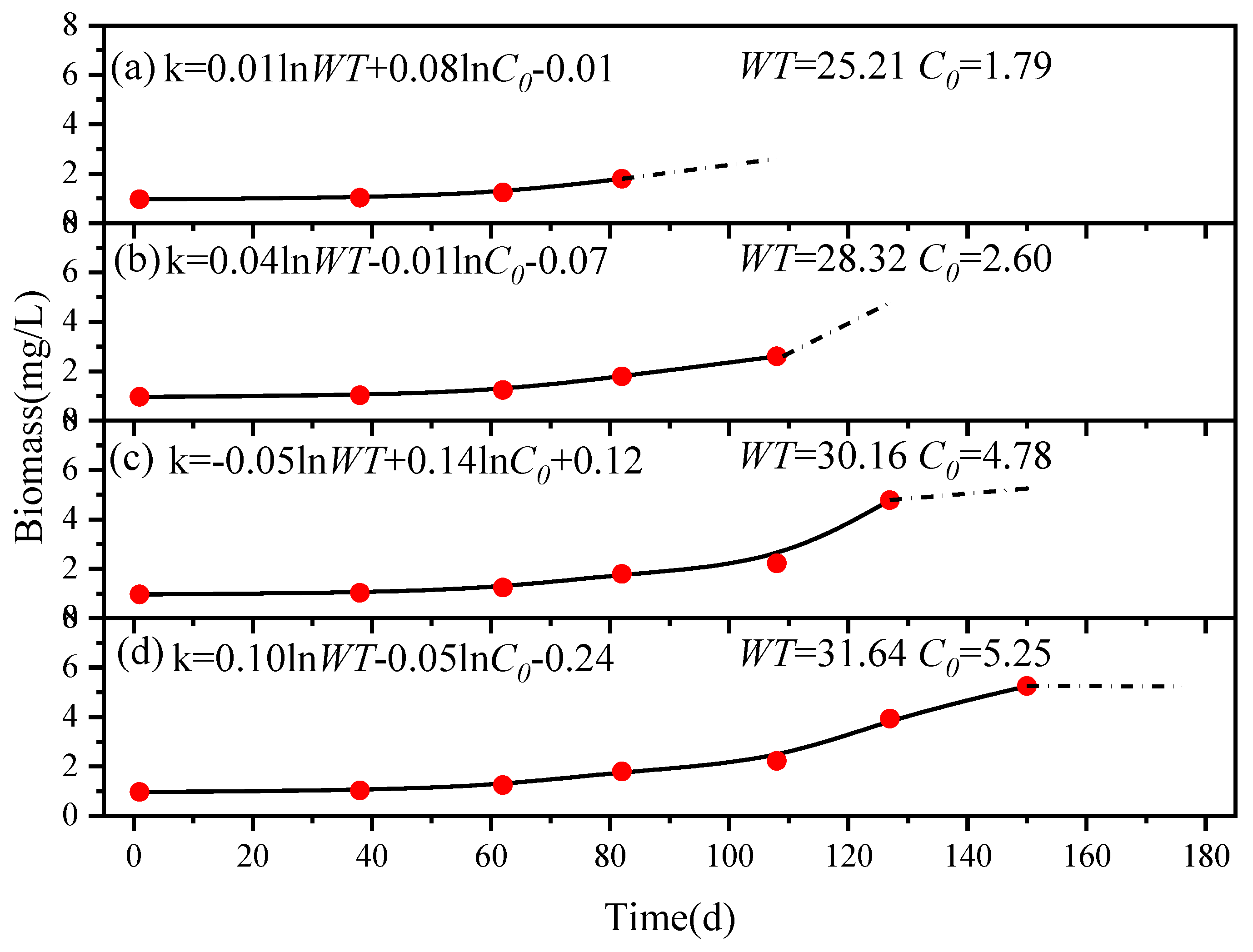
Using sampling point S4 as an example, we predicted the future growth of algae (Figure 7). The input data used for training the model included the preceding four monitoring records. Equation (4) was employed to conduct regression calculations on the growth rate coefficient (k), offering the following calculation equation for the growth rate coefficient in the subsequent stage:

$$k=0.01\ln \left(WT\right)+0.08\ln \left(C_0\right)-0.01$$

(8)

where WT is the average water temperature during the target prediction period, which was determined using Equation (5) and the temperature data gathered from the previous 26 days’ weather forecast. C₀ is the initial biomass concentration obtained from measuring the biomass at the initiation of the prediction period (Day 82). By employing this equation, it became feasible to calculate the growth rate coefficient (k) for the desired time. The resulting k was subsequently employed in the established logistic model to derive the algal biomass for the subsequent 26 days (Day 108).

Upon acquiring the actual monitoring results for Day 108, the model was evaluated to assess its accuracy. The monitoring result served as the initial biomass concentration, and Equation (4) was utilized once more, along with the predicted water temperature, to estimate a fresh k employed in predicting the biomass for Day 127 (60 days after the start). This iterative process persisted, allowing the model to make predictions of the biomass throughout the entire algal growth period by consistently acquiring monitoring data and temperature predictions. Subsequently, the model’s predictions were continually refined through a comparison with the actual monitoring results, consequently leading to improved prediction accuracy.

The model’s predictions for Day 108, Day 127, Day 150, and Day 176 were 2.60 mg/L, 4.78 mg/L, 5.25 mg/L, and 5.24 mg/L in consecutive stages. The corresponding monitoring yielded values of 2.22 mg/L, 3.93 mg/L, 4.90 mg/L, and 5.20 mg/L. The model demonstrated high prediction accuracy for sampling point S4.

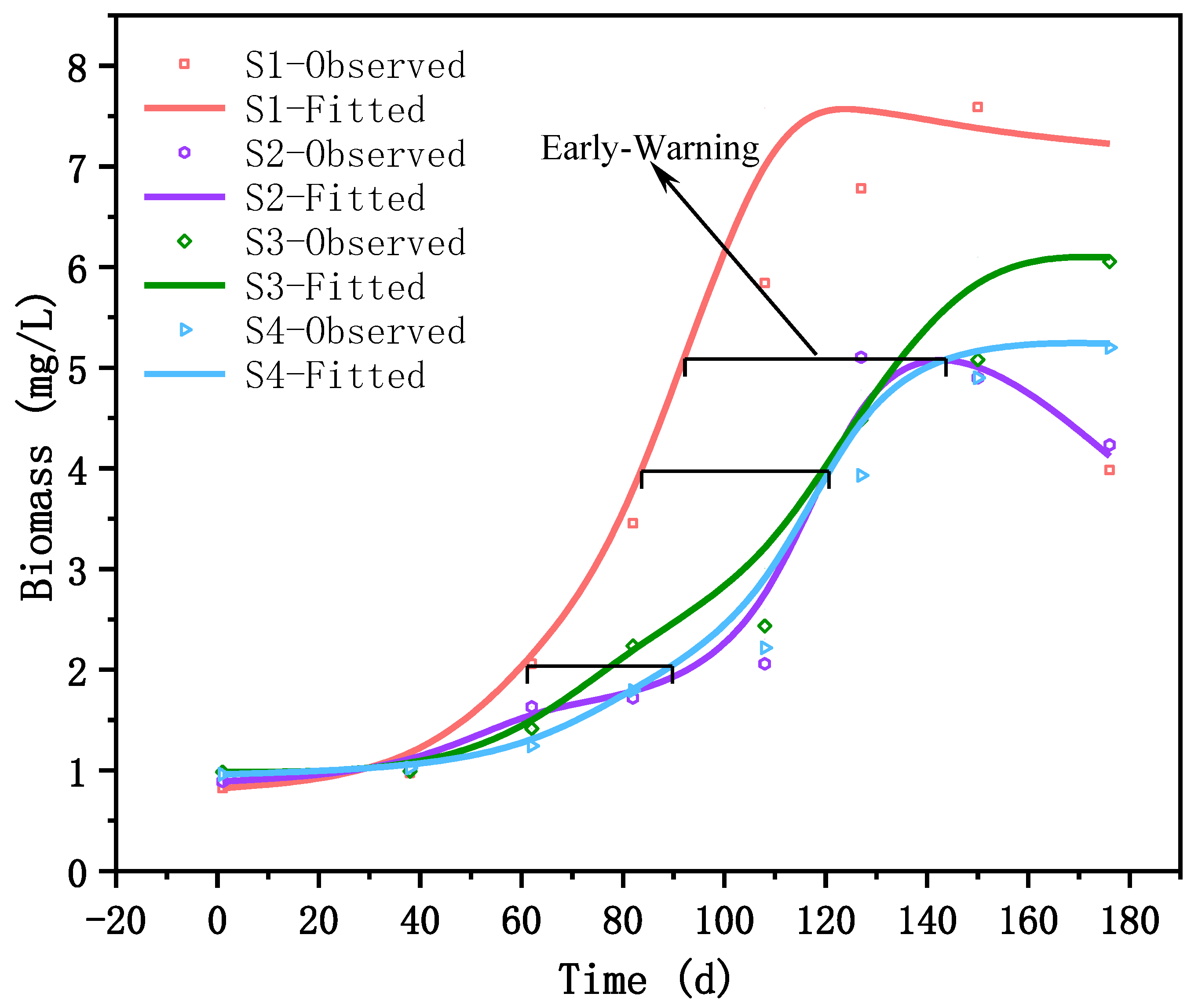
The application of this approach to predict sampling points S1 to S4 revealed the model’s ability to discern the spatial disparities among the four sampling locations in the Nanwan Reservoir. The coefficients of determination (r-squared) for the observed and predicted values were as follows: r_S1² = 0.6581, r_S2² = 0.9793, r_S3² = 0.9142, and r_S4² = 0.9391 (Figure 8).

3.4. Long-Term Prediction of Algal Biomass in Drinking Water Intake Area

According to the predictive results, the biomass of algae in the inflow area of the Wudaohe River in the Nanwan Reservoir exhibited the earliest exponential growth phase, characterized by a higher growth rate. The inflow area of the reservoir is relatively shallow in comparison to the central region, rendering it more susceptible to water temperature fluctuations (Figure 5). This area showcased greater responsiveness to temperature changes during the season of rising water temperatures, thereby resulting in accelerated algal growth when compared to other regions. Furthermore, the accumulation of algae was more pronounced in the inflow area compared to other parts of the reservoir. These factors collectively contributed to the elevated biomass levels observed in the inflow area.

The biomass in the inflow area reached a concentration of 2 mg/L on Day 60, whereas the water area in front of the dam reached the same concentration 30 days later (Figure 8). There was a time difference of 40 days between the two areas, reaching a concentration of 4 mg/L, and as time progressed, the water area in front of the dam reached a concentration of 5 mg/L 50 days after the inflow. The algal biomass in the inflow area of the reservoir gradually increased, following a growth trend similar to that observed in the above area. These results suggest that the growth trend of algae in the inflow area can be utilized to forecast algal growth near the water intake in front of the dam with a minimum of 30 days’ notice. By incorporating the 30-day prediction of algal growth in the inflow area and utilizing the inflow as the reference point and the water intake in front of the dam as the target, attaining a minimum of 60-day early warning capability became viable.

This study focuses on the Nanwan Reservoir, with the ultimate goal of forecasting algal biomass. By calculating the relationship between air temperature and water temperature, monitoring biomass, and implementing self-correction in the model, we successfully achieved a 30-day advance prediction of algal growth in the reservoir. The model demonstrated high prediction accuracy and provided a minimum 60-day early warning capability for the water intake area in front of the dam. This was achieved using the upstream inflow area as the reference point. However, the final biomass of algae in different reservoirs is influenced by multiple factors. Therefore, it is necessary to make adjustments to the key factors and their values based on specific circumstances when implementing the model. However, this study does not consider the impact of community succession on the prediction results when using algal biomass as the forecasting target. Future research can enhance the generality and accuracy of the model by performing parameter optimization and incorporating growth weights specific to different algal species.

4. Conclusions

The algal biomass in the Nanwan Reservoir showed seasonal variations, primarily influenced by water temperature (p < 0.05). The AWAM model was developed by incorporating water temperature and initial biomass concentration into a logistic model. Utilizing four monitoring data points, a 30-day prediction of algal biomass was achieved, overcoming the limited data availability. The model continually refined itself based on the latest monitoring results, resulting in accurate predictions (R² = 0.74). The predictive results of algal biomass in different zones of the reservoir indicated that the model could accurately forecast algal growth in various regions. The growth of algae in the water intake area in front of the dam exhibited a delayed onset compared to the inflow area of the Wudaohe River tributary. Additionally, using the inflow area of the upstream river as a reference point, the model could provide a long-term prediction for the water intake area in front of the dam with a lead time of at least 60 days.