1. Introduction
Reservoir characterization is essential for oil-field management [
1,
2], such as production optimization and uncertainty analysis, which aims to inverse uncertain geological properties (i.e., the permeability field). The petrophysical parameters obtained by well logging can reflect the geological properties around the well. The petrophysical properties are very heterogenous in the real reservoir, which means the parameters acquired by the sampling points of well logging are difficult to use to reflect the whole characteristics of a continuous area. Thus, instead of inversing the physical properties of limited points, reservoir connectivity characterization could quantify the relationship between injectors and producers and thus infer the underground high-flow channels [
3]. However, the description of interwell connectivity is a big challenge due to the great uncertainty and heterogeneity of a petrophysical property. The commercial simulators enable revealing the communications between injectors and producers through gridding calculation [
4]. Subsurface geological properties are essential for the development of simulation models, which are quite difficult and expensive in practice. Besides, the higher the number of grids, the more computational resources the commercial simulators cost [
5]. To make the inter-well connectivity analysis easy to implement, a variety of injection–production data-driven methods are proposed.
Physical models are one group of mainstream data-driven approaches for the measurement of interwell connectivity. The capacitance resistance model (CRM) [
6] is derived from the material balance equation and the linear productivity prediction model, reflecting the connectivity between injection and production wells via their rate fluctuations. Based on the similarity between the hydraulic system and power system, CRM uses weights and time constants to quantify the connectivity (capacitance effect) and signal lags (resistance effect) of each injector–producer pair. A series of variants of CRM have been proposed and utilized in different cases in the last decade [
7]. For instance, to improve the accuracy of reservoir property characterization, Naudomsup et al. [
8] integrated CRM with the injection data of tracers. Additionally, combined with the Y-function method, a Buckley–Leverett-based waterflood analysis model, CRM can further strengthen the robustness [
9]. Comparatively, the inter-well numerical simulation model (INSIM) is another category of physical methodologies [
10], developed with the material balance equation and Buckley–Leverett theory. By simplifying the waterflooding reservoir into a series of volume flow units, INSIM can accelerate the simulation process and characterize the permeability channels of injector–producer pairs. Based on INSIM, several improved versions have been proposed, such as INSIM-FT-3D [
11] simulating the waterflood in three dimensions and considering the gravity effect and INSIM-FPT [
12] replacing the reservoir properties by history matching results. Additionally, Lee, Ortega, Nejad, Jafroodi, and Ershaghi [
13] proposed that the waterflooding reservoir can be regarded as a multiple-input multi-output (MIMO) system. Combined with the finite impulse response (FIR) method, they put forward a linear FIR-MIMO system to characterize fractures and high-permeability channels, only using injection and production rates. Physical models have strong reliability and interpretability, because they are established on the solid foundation of seepage mechanics. The development process for these physical models is rather complicated, demanding a lot of expert knowledge in reservoir engineering.
As another important category of data-driven methods, machine-learning-based approaches have received continuous attention [
14,
15]. Different from physical methods, machine learning approaches can match the production history and infer the injection–production relationship using their significant nonlinear mapping ability instead of physical principles. Artun [
16] utilized the product of the weight matrices of a single hidden-layer feedforward neural network to reveal the interlink between injection data and production data. Du et al. [
17] employed a convolutional neural network (CNN) and backpropagation neural network (BPNN) to infer the inter-well connectivity via oil production, injection pressure, and water cut, and permeability data were required for the training process. Moreover, the sensitivity analysis technique can also be employed in neural networks to reveal the relationship of injector–producer pairs [
18]. Compared with physical methods, machine learning approaches are much easier to build, requiring less professional knowledge. However, one vital disadvantage of machine learning methods is that their model parameters are unexplainable, since physical knowledge is not considered in the model design process. Furthermore, to maintain a stable performance on different learning tasks, the inheritability and generalization ability of machine learning models have to be guaranteed. For these challenges, the reliability of these machine learning methods is always doubted in practical applications.
Associating physical knowledge with machine learning models is an effective way to improve generalizability and interpretability. A physics-guided neural network (PGNN) [
19] has been successfully applied in simulating a lake’s temperature, using the results of physical models and leveraging physical rules to improve the scientific consistency of neural networks. Raissi et al. [
20] associated the partial differential equation (PDE), boundary condition (BC), and initial condition (IC) as the objective function of networks, named physics-informed neural networks (PINN). In addition, physics-informed deep neural networks showed robust performance in forecasting the parameters and constitutive relationships in subsurface flow through minimizing the PDE (Darcy or Richards Equation) residual [
21]. Furthermore, a theory-guided neural network (TgNN) [
22] was proposed to calculate the subsurface flow process, taking into account not only PDE, BC and IC but also expert knowledge and engineering controls. Basically, these methods associate the physical knowledge with the objective function in the form of regularization terms, thus forcing the neural networks to make predictions within certain physical constraints. However, the introduction of penalty terms inevitably leads to the increase in hyperparameters, which are difficult to determine and negative to the model stability. To solve these problems, we aim to fuse the physical knowledge in an alternative way, such as constructing model blocks with specific physical functions.
To improve the model inheritability, transfer learning has been utilized in plenty of learning tasks with certain similarities [
23]. In the petroleum area, Yin et al. [
24] associated genetic transfer learning with the surrogate model to optimize oil production, significantly strengthening global research capability by transferring cheap information from low-fidelity results to tackle the high fidelity tasks. Based on a transfer learning framework of the random forest method, the assessment of undeveloped fields can be better forecasted by using the model trained on the data from mature fields [
25]. In addition, in the image classification field, Zhang et al. [
26] put forward transferring the structures learned by deep convolutional neural networks from other subjects to new target ones, thereby improving the classification accuracy of electroencephalography (EEG) data. In the work of [
27], an adversarial neural network with class-weights employed partial transfer learning to enhance the diagnostic knowledge utilization efficiency in machine fault diagnosis problems. Furthermore, an attentive feature alignment (AFA) approach was adopted in transfer learning transfer by focusing on the spatial features and correlation channels, which demonstrated great generalization capability on several face recognition datasets [
28].
The hybrid approaches can usually obtain a balance between approximation accuracy and computation cost, by combining the advantages of different methodologies [
29,
30]. Inspired by these works, we embed the material balance equation in a network via several transparent blocks, called a physical knowledge fusion neural network (PKFNN). PKFNN aims to characterize the connecting relationship between each injector and each producer by the physical evaluation function and forecast the behavior of producers. We note that the productivity is not only determined by the injection wells but is also influenced by different producers. Therefore, transfer learning is used in PKFNN to improve knowledge utilization efficiency by mapping from the source domain of other producers to the target domain of the analyzed producer. We tested the performance of PKFNN on inferring inter-well connectivity by three simulation experiments, demonstrating the effectiveness and efficiency of the proposed method.
The major contributions we deliver in this paper are listed as follows:
- (1)
A novel neural network named PKFNN is developed, cooperating with ODE (the material balance equation) to control the approximation of the waterflooding process, thereby revealing the physical principle of the data and guaranteeing the rationality of estimation.
- (2)
A physical evaluation function is built to ensure the physical boundaries of inter-well connectivity and avoids the complex computation resulting from constraint optimization.
- (3)
The physical knowledge transfer and model structure transfer are employed in PKFNN to cope with the continuity and homogeneity of geological properties, increasing the interactions between models.
The remainder of this article is organized as follows. In
Section 2, we introduce some preliminaries (transfer learning and inter-well connectivity analysis) of PKFNN. Then we provide a detailed description of model architectures and workflow of PKFNN in
Section 3. In
Section 4, we test the effectiveness of PKFNN through four reservoir simulation experiments. Finally, we summarize this article and obtain some conclusions in
Section 5.
3. Physical Knowledge Fusion-Based Neural Network (PKFNN)
For typical neural networks, the connecting weights between synapses cannot be interpreted intuitively, so they are called “black box” models. To enhance the model transparency and interpretability, we expect to construct a block-based neural network, wherein different blocks are designed to realize the extraction and mapping of different features. Furthermore, the framework of PKFNN should be developed on the first principle of the analyzed physical problem, which is the ODE (material balance equation) of the flow among the reservoir. In our work, PKFNN is composed of the knowledge-distillation block and the mapping-transfer block. In the knowledge-distillation block, a physical evaluation function is designed to indicate the connecting strength of each injector–producer pair. The values of the physical evaluation function are multiplied with the vectors of WIR, to compute the total water flow-in rate toward the analyzed producer. Since the range of the proposed function is [0, 1], the physical constraints of the connectivity analysis can be guaranteed. To decrease the multiplicity of the connectivity characterization, Pearson’s correlation coefficient method is applied in the initialization process. Furthermore, the sparse characteristics of the physical evaluation function further enhance the stability of the interwell connectivity characterization. The mapping-transfer block is constructed to approximate the fluid change rate among the control volume, and we would provide the detailed deduction in
Section 3.2. By the nonlinear activation function and complex connecting neurons, this block can find the nonlinear mapping relationships between the input signals to the estimated signals in a high-dimensional space. Due to the continuity and homogeneity of the reservoir, the fluid change rates among the control volumes of different producers should also have some similarities. Therefore, the transfer learning algorithm is employed in this block to transfer the learned topological structures from the previously trained model. In this way, the effects of water injection, the fluid change rate of the control volume caused by compressibility, and the interlinkage between injector–producer pairs can be accounted for in PKFNN with the knowledge-distillation block, the mapping-transfer block, and transfer learning. The studied cases have proven that this transfer learning scheme can effectively speed up the model convergence rate. Based on the outputs of the above two blocks, PKFNN can estimate and forecast LPR or water cut, according to the material balance equation. The abbreviation and subscripts used in this paper is listed in
Appendix A.
The material balance equation employed in PKFNN operates under the following assumptions: (1) the fluids only contain oil–water in two phases, (2) the reservoir pressure is above the bubble point, (3) the reservoir temperature is constant, (4) both the porous media and fluids are slightly compressible.
3.1. Knowledge-Distillation Block
The characterization of the relationships between injection and production signals reflects the relative connecting strength of each injector–producer pair, which is nonnegative and in the range of 0 to 1. To distill this physical knowledge by PKFNN, a physical evaluation function is put forward in this block, aiming to measure the contribution from all possible connecting injection wells to the analyzed production well.
Assume that the input data are WIRs of
M injector,
I = [
i1,
i2, …,
im, …,
iM]
T. Followed with the input signals, the physical evaluation is constituted for the evaluation of the contributions between each injector to the considered producer. Summing the dot product of the given input vectors and their corresponding physical evaluation values, the output of the knowledge-distillation block yields:
where
denotes the total injected water-flowing rate from all injectors toward the producer
o;
is the physical evaluation employed to measure the contribution from injector
m to producer
o, where
is the independent variable of the physical evaluation that needs to be optimized.
The motivation for using physical evaluation to infer inter-well connectivity comes from the work of feature selection by Chakraborty and Pal [
32], who used the values of this function to measure the importance of input variables. Chakraborty and Pal mentioned that the gate function might be any monotonic differentiable function in the range [0, 1]. We employ a composite exponential function as the physical evaluation function in the proposed model due to its stability and efficiency. The idea of the physical evaluation method is simple. Each input variable would be assigned to a physical evaluation as a coefficient, and the function value would update in the training process. If a variable is vital for the learning task, its function value would be relatively bigger than other less-important ones after the training. In other words, the value of this physical function can be recognized as a gate, which would be opened for important variables and closed for variables contributing weakly to the learning task. Similarly, the injectors that strongly connect with producers make great contributions to oil production, so their physical evaluation function values would also be big when the training is finished and vice versa. Assume that there are
M injectors and
O producers, the physical evaluation function used in PKFNN is defined as:
where
is the connectivity matrix.
The physical evaluation function resolves two important problems in the inter-well connectivity characterization problems, the multiplicity, and the nonnegative constraint. The essential precondition of the correct reservoir characterization is that the productivity can be matched with certain precision, and this process is named history matching. However, as a typical inversion problem, inter-well connectivity analysis has strong uncertainty, which means different connecting characterization results may generate similar history-matching precision. To tackle this issue, we propose using the statistical information of injection–production data to help PKFNN initialize its physical evaluation function. Because these statistical approaches, like Spearman rank correlations [
33] and Pearson’s correlation coefficient method [
34], have been proven to reflect the inter-well connectivity. Specifically, PKFNN uses the Pearson correlation method to initialize
(the independent variables of
):
where
I = [
i1,
i2, …,
im, …,
iM]
T denotes the WIRs of
M injectors, and
Q = [
q1,
q2, …,
qo, …,
qO]
T is the LPRs of
O producers;
and
are the Pearson correlation coefficients and the covariance matrix calculated from
I and
Q;
,
represent the standard deviations of
I and
Q, respectively.
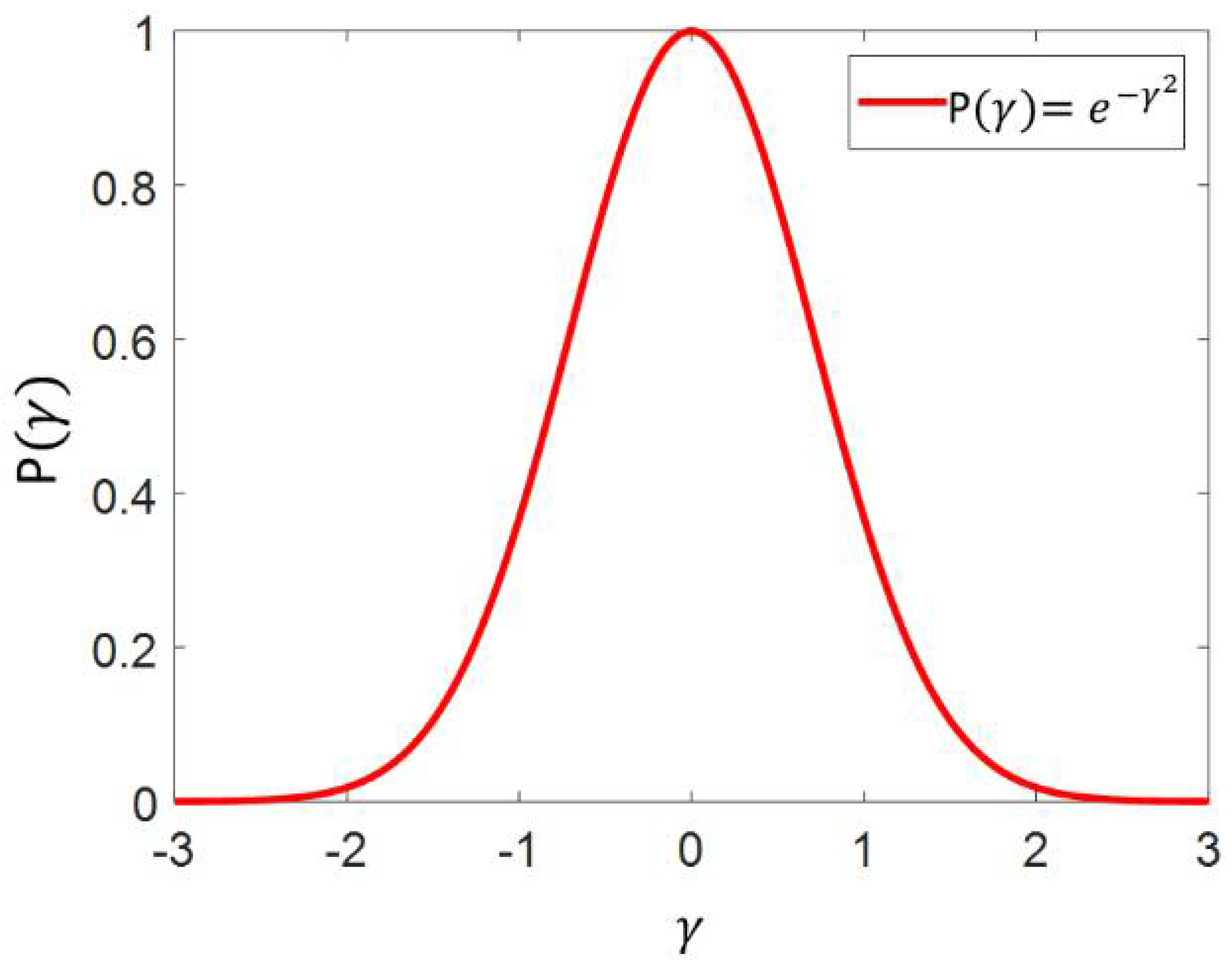
Through this specific initialization method, an injector–producer pair with a high correlation relationship would obtain a big gate value, and vice versa. Therefore, this Pearson-correlation-coefficient-based initialization method would help ICM start optimization from a small parameter range close to the real connecting conditions. Except for the initialization method, the sparsity of the physical evaluation function enables the further reduction of the multiplicity. As shown in
Figure 1, only if
is in a limited range (between −1 and 1), the proposed physical evaluation function can produce relatively bigger values, while the values would be restricted to be small in other areas. Obviously, this exponential sparse function would keep the inter-well connectivity characterization results much more stable than the linear coefficient evaluation method.
Another advantage of this physical evaluation function is that its range is strictly limited between 0 and 1, ensuring the explicit physical significance of the function values. Hence, in the knowledge-distillation block, can be upgraded by any gradient-based optimization algorithms without constraints. This merit guarantees the high computation efficiency of PKFNN.
3.2. Mapping-Transfer Block
The mapping-transfer block employs an artificial neural network to estimate the fluid change rate of the control volume among the considered producers. Moreover, the model structure is inherited from the previously trained blocks, significantly reducing the computation cost during the optimization process of PKFNN. This block is established on the assumption of a nonlinear productivity prediction model, which can be expressed as:
where
represents the nonlinear mapping relationship. Significantly, the average pressure of the control volume,
, is often unavailable, so we change the independent and dependent variables in Equation (9):
where
F is another mapping differentiated with
. The differential equation of Equation (10) is given by:
Considering the case with constant BHP (the most common production scheme in practice), Equation (11) can be simplified as:
Then, the fluid change rate among the control volume can be calculated by multiplying
to the left and right sides of Equation (12):
To evaluate the influence of
M injectors on the control volume, Equation (13) can be extended as:
where
NN denotes the nonlinear mapping by the layers. Herein, we utilize an approximation between
and
. It should be noted that
can be eliminated, since these two parameters are usually considered constants, which can be included in the weights of networks.
Furthermore, the pressure among the control volumes is also affected by water injection, and the variable BHP of producers is due to some operations, such as lifting pumps and structural elevations. Therefore, considering the production with variable BHP, and the BHP data of injectors are available, the fluid change rate among the control volume can be approximated by the nonlinear mapping of injectors’ BHP,
, the analyzed producer’s BHP and LPR,
, and
. Thus, Equation (14) can be extended as:
3.3. Model Framework and Learning Strategy
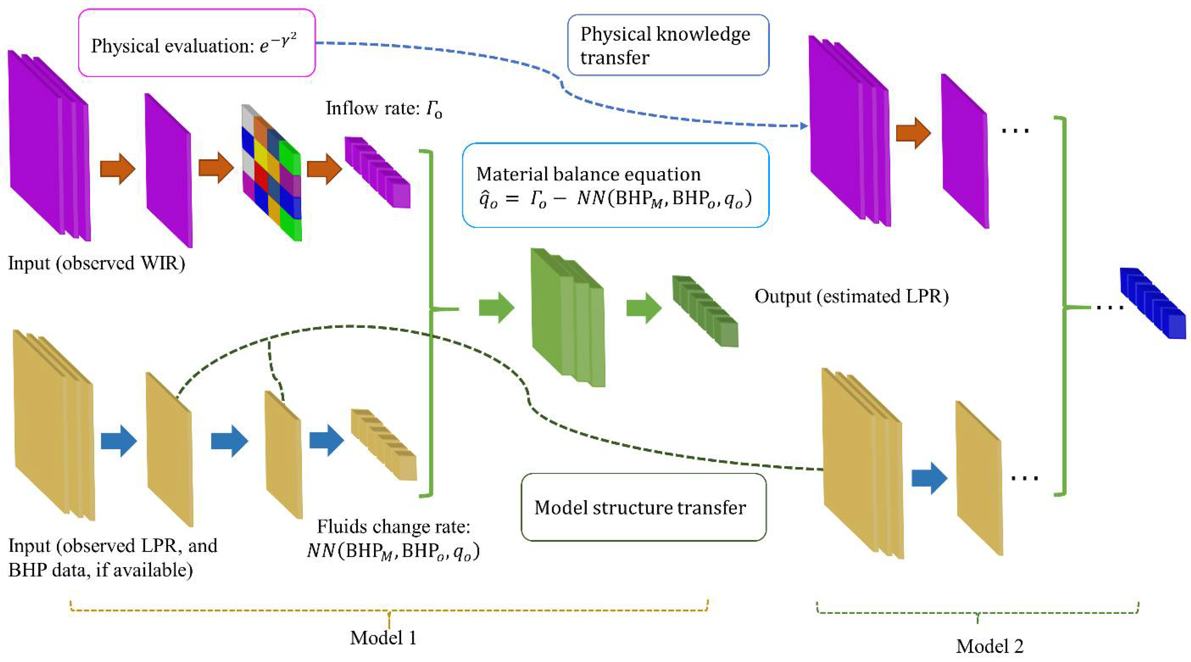
Based on the framework material balance equation, PKFNN associates the injection and mapping-transfer blocks, characterizing the injection–production relationship and forecasting productivity. As shown in
Figure 2, the input data of PKFNN consists of two parts, including the observed water injection rate (WIR) for the knowledge-distillation module and the liquid production rate (LPR), and BHP data (if available) for the mapping-transfer block. In the knowledge-distillation block, we utilize the WIR data and physical evaluation function to calculate the total inflow rate of the analyzed producer, according to Equation (5). Meanwhile, the injection–production relationship would be extracted via the evaluation function. In the mapping-transfer block, a neural network is employed, approximating the fluid change rate of the control volume through LPR data. Actually, the two blocks are designed to extract the physical features from input data, and the block structures are assigned to clear the physical sense. After the feature mapping of these two blocks, considering the constant producing BHP, the material balance equation is used to integrate two blocks to calculate the estimated LPR, which can be given as:
Considering the variable producing BHP, Equation (16) can be expressed as:
where
denotes the estimated LPR for the considered producer. The mean square error (MSE) function is used as the loss function:
where
t is the time step, and
T denotes the number of total time steps. In this framework, PKFNN guarantees that, for each producer, the production rate equals the difference between the total inflow rate minus the fluid change rate within its control volume.
To make full use of the knowledge in the dataset and improve the generalization capability of PKFNN, we present physical knowledge transfer and model structure transfer in PKFNN’s optimization, as shown in
Figure 2. The transfer learning strategy is demonstrated in
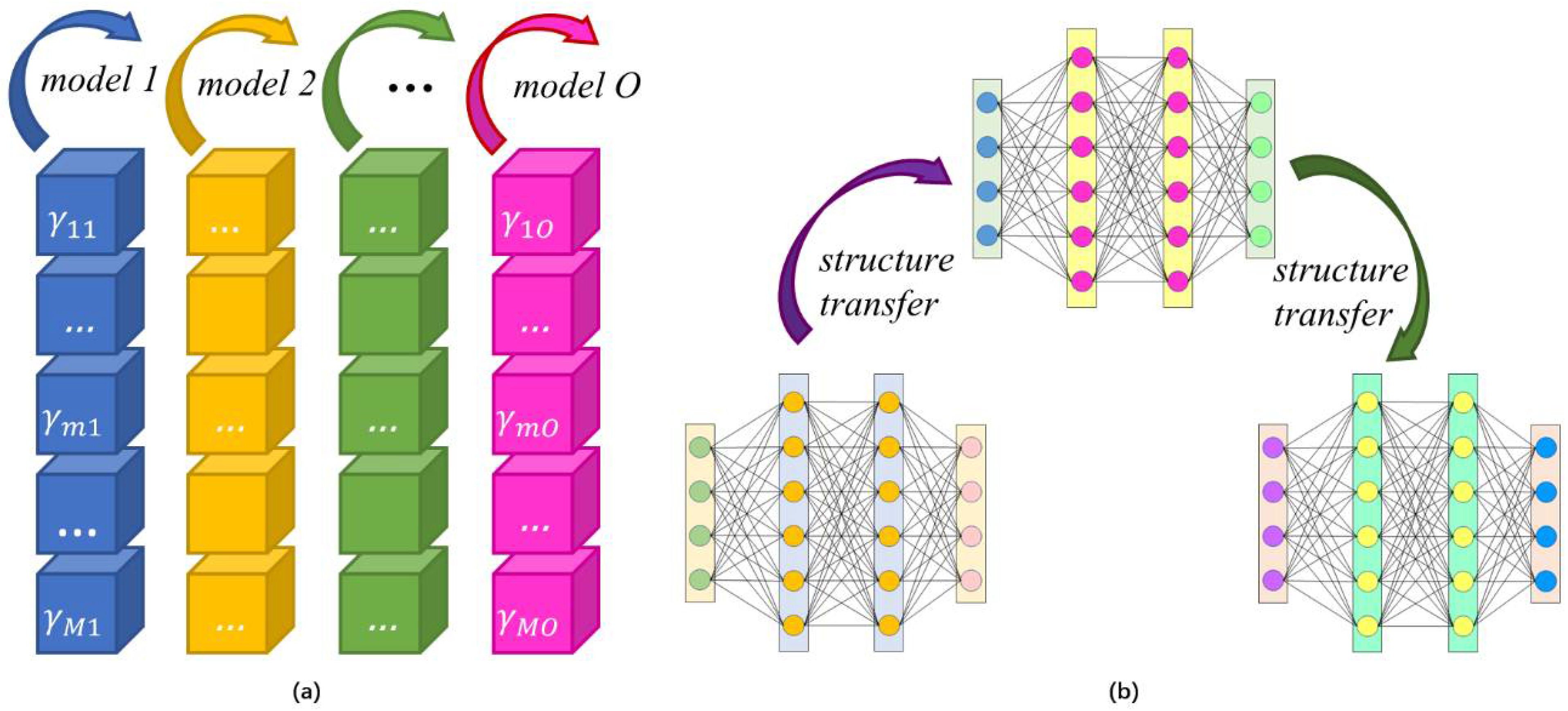
Figure 3. As shown in
Figure 3a, the physical knowledge is transferred from the Pearson correlation reciprocal matrix to the independent variables of the physical evaluation function. This physical knowledge can be transferred as there is a tight interlinkage between the Pearson correlation coefficient and the proposed physical evaluation functions. On the one hand, the Pearson correlation coefficient can measure the linear relationship between the injection signals and production signals, wherein the more correlative of two signals, the bigger their coefficient. On the other hand, the designed physical evaluation functions can initialize the independent variables with the knowledge of the correlation matrix. For instance, if one correlated injector–producer well pair obtains a big value by the Person correlation method, the absolute value of its reciprocal would be small, and it would generate a large value through the nonlinear transformation of the physical evaluation function, as illustrated in
Figure 1. In this way, the transfer of physical knowledge could reduce the uncertainty of interwell connectivity characterization significantly. The model structure also adapts the transfer learning in the mapping-transfer block. In the training process, PKFNN is established on each producer and its possible connecting injectors successively. As shown in
Figure 3b, when the first model has finished learning, the connecting weights of the network in the mapping-transfer block would be transferred to the second model, and so on. Herein, for
O analyzed producers, we use {
,
, …,
, …,
} and {
,
, …,
, …,
},
to denote the initial and trained parameters (connecting weights) of the mapping-transfer block, respectively. The structure transfer learning used in neural networks is given as:
Affected by the continuity of sedimentary facies, the physical parameters in the same oil reservoir usually show a certain similarity. During the waterflood recovery process, there are also some kinds of affinities in different production wells for the homogeneity of the reservoir. The motivation for the model structure transfer depends on the isotropy of the geological properties, and the oil reservoir is under the same pressure system, which means the average pressure of , , of adjacent producers may have a similar trend. As Equation (13) shows, the fluid change rate of the control volume is the differential of concerning , hence the learning task of the approximation of enables it to be transferred between models. PKFNN is developed on each producer and all possible connected injectors, so the new model can inherit the structure from the trained model and converges fast after fine-tuning.
The pseudocode of the PKFNN training process is shown in
Algorithm 1. Based on WIR and LPR data and the BHP data (if available) of injectors and producers, PKFNN aims to approximate and forecast the productivity of producers and characterize the inter-well connectivity. First of all, for each producer from 1 to
O, the physical evaluation function is initialized by Equations (6) and (8). In this way, the multiplicity of the inter-well connectivity characterization can be reduced by transferring the physical information in the knowledge-distillation block. Moreover, the model structure transfer learning is applied in the mapping transfer block to inherit the weights learned from the target domain. For the first model, the initialized connecting weights obey the normal distribution with 0 mean value and 0.25 variance,
(0, 0.25). When the history matching task is finished, the optimized weights would be transferred to the second model, according to Equation (19), and so on until all models finish training. Thus, the topology structures learned from the source domain can be inherited from the current model in the target domain. In this process, the injection data are in both the source task and the target task, and the production data (BHP data and liquid production rate data) are selected according to the analyzed producer. Then, the outputs of the knowledge-distillation block and the mapping-transfer block can be calculated by Equations (5) and (13) (or Equation (14)), respectively. Next, the model output can be generated by the material balance equation, Equation (16) (or Equation (17)), and the model loss can be computed by Equation (18). Finally, the network weights,
, and the independent variables of the physical evaluation function,
, can be optimized by their gradients with respect to the loss function.
| Algorithm 1. Pseudocode of PKFNN training process. |
| /Start PKFNN training/ |
| For o = 1 to O do |
| While stop criteria is not met |
/Physical knowledge transfer/
Initialize physical evaluation function using the column, , according to Equations (6) and (8); |
/Model structure transfer/
If
Initialize obeying normal distribution (0, 0.25);
Else do
Assign to , according to Equation (19); |
/Knowledge-distillation block calculation/
Calculate the total injected water flowing rate, , according to Equation (5);
/Mapping-transfer block calculation/
Constant producing BHP case: calculate the fluid change rate of byEquation (13);
Variable producing BHP case: calculate the fluid change rate of byEquation (14); |
/Loss evaluation/
Generate the model output byEquation (16) (or Equation (17));
Calculate the loss function using Equation (18); |
/Parameters update/
Update and via their gradients with respect to the loss function, Equation (18).
End if
End while
End for |
| /End PKFNN training/ |
3.4. Productivity Forecast
When PKFNN has learned the connecting relationship of each injector–producer pair, it can be used to predict the productivity behavior of production wells. Basically, productivity forecast can be regarded as the test procedure of PKFNN, illustrating the generalizability of the proposed approach. Since all parameters of PKFNN are constants after training, the only unknown liquid production rate
can be predicted by solving the following equation:
4. Results
To prove the effectiveness of the proposed approach, three synthetic reservoir cases, named the eight-injector–eight-producer case, the braided river case, and the Egg case, and one benchmark case, the Brugge field case, are constructed on ECLIPSE (Schlumberger Ltd., Houston, TX, USA), providing the dataset for the inter-well connectivity characterization and productivity forecast. The synthetic reservoir models established by ECLIPSE are assumed to conform to the seepage physical laws. Thus, given a certain well-control schedule to the simulator, it can calculate the corresponding WIR and LPR signals, in line with the material balance equation for the waterflooding process. The first three cases are the 2D models and the Brugge field case is a 3D model with nine layers. In the first two synthetic cases, the permeability fields are relatively simple, and the production is under the condition of constant wellbore pressure. Thus, only the WIR and LPR data are used in PKFNN for history matching, production prediction and reservoir connectivity characterization. In
Section 4.1, the eight-injector–eight-producer case is implemented with four high-permeability streaks and the homogenous permeability matrix. In
Section 4.2, the braided river case is tested, which is a reservoir model with common fluvial deposition of the continental facies basin. There are five injectors and four producers in this case, and the permeability values of the river courses and the matrix are 500 md and 5 md, respectively. The last two simulation cases take the changing wellbore pressure production schedule, so the BHP data of both injectors and producers are fed to PKFNN. In
Section 4.3, there are eight injectors and four producers in the Egg case, which is a fluvial sandstone reservoir with very heterogeneous permeability. The SPE benchmark case, the Brugge field case is tested in
Section 4.4, which is a true oil-field production case with actual injection and production schedules.
In this paper, in chronological order, the former 70% and the latter 30% data are adopted as the training and testing data, respectively. The hyperparameters of PKFNN used in three cases are demonstrated in
Table 1, where
(0, 0.25) represents the normal distribution with 0 mean value and 0.25 variance. The history-matching and prediction results of the water cut are provided in our work. Similar to the estimation and forecast process of LPR, the water cut can be handled by only replacing the LPR data with water-cut data.
4.1. 8-Injector–8-Producer Case
As shown in
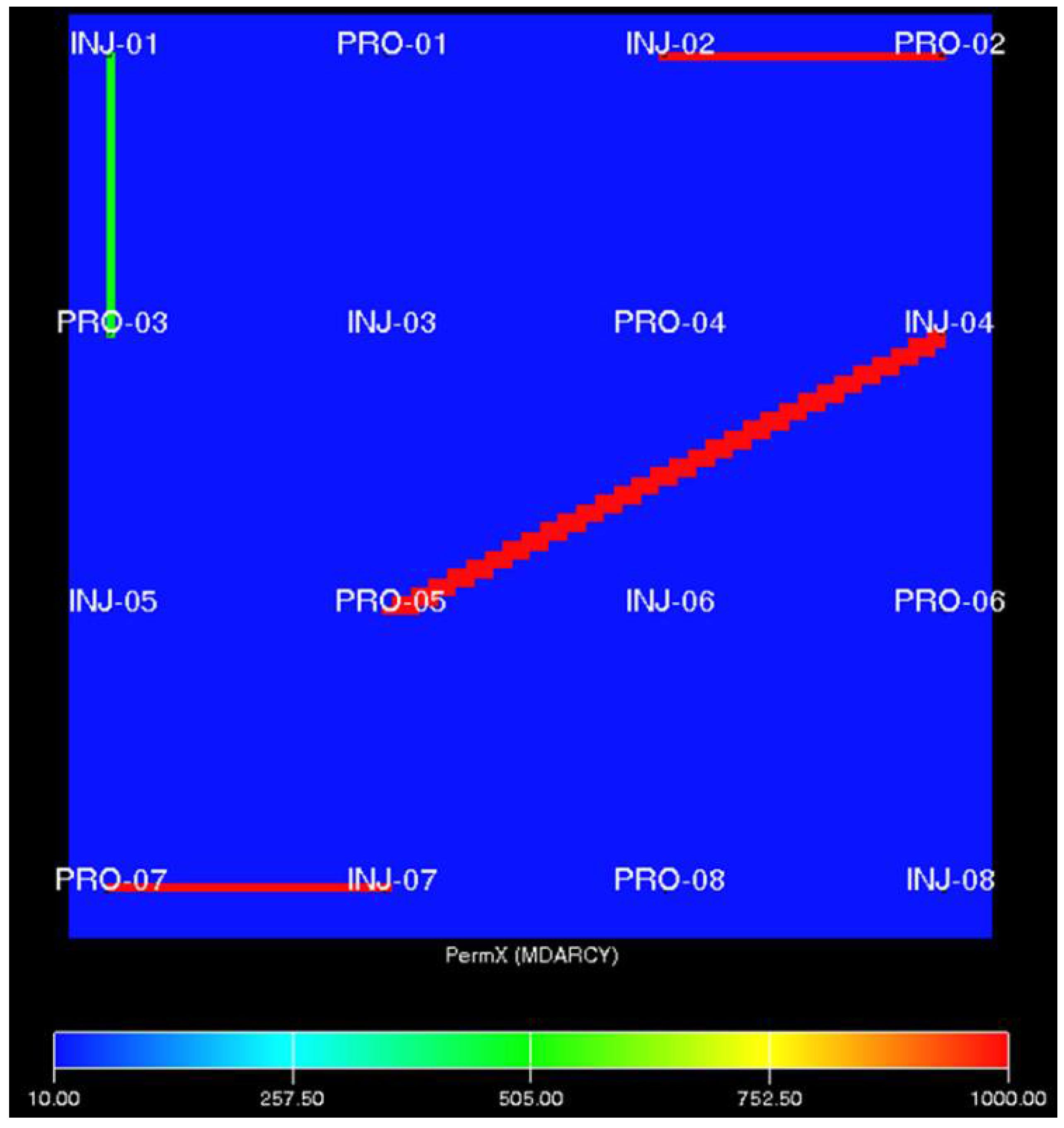
Figure 4, there were 8 injectors and 8 producers in this simulation case, consisting of 100 × 100 × 1 grids, with 75, 75 and 10 ft in the
X,
Y, and
Z axes, respectively. In this case, four high-permeability streaks connected four injector–producer pairs, INJ-01–PRO-03, INJ-02–PRO-02, INJ-04–PRO-05, INJ-07–PRO-07, separately. The permeability of the reservoir matrix was 10 md, and except for the streak between INJ-01 and PRO-03 being 500 md, the other three streaks were 1000 md, and the detailed properties are listed in
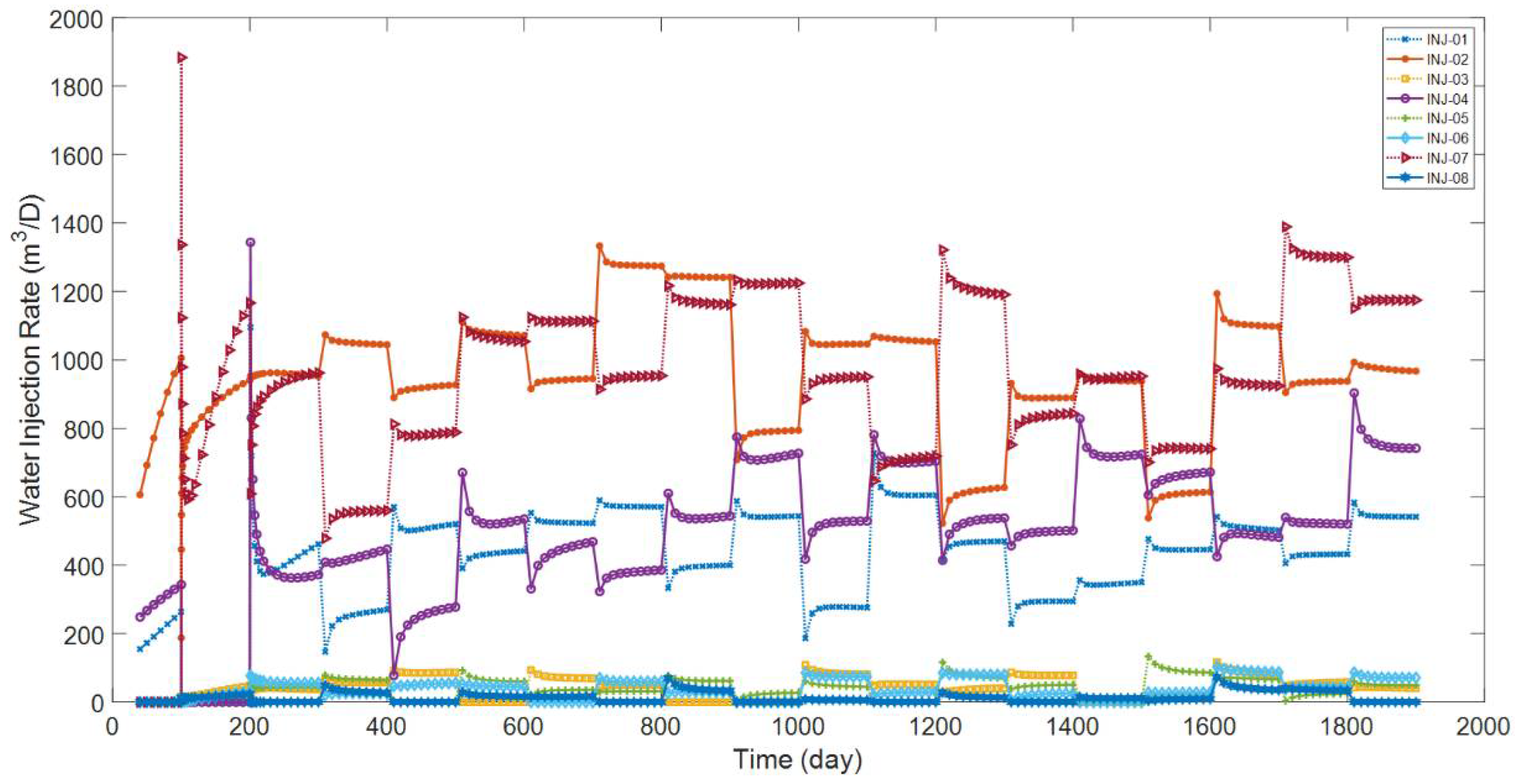
Table 2. During the production periods, the BHP of the eight producers remains constant. The simulation lasted 1900 days, and the time step was 10 days.
The water injection rates of eight injection wells are shown in
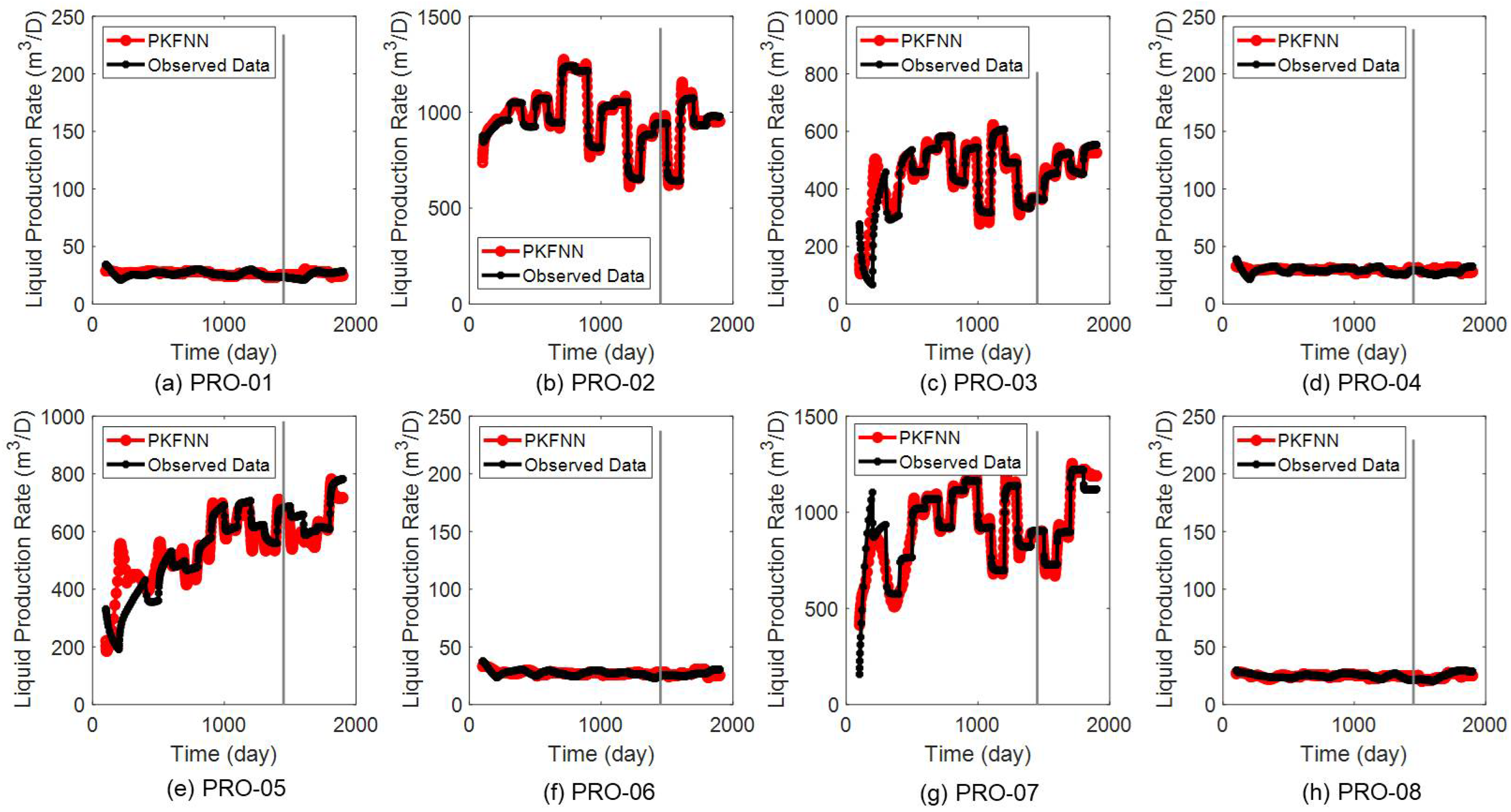
Figure 5, which remain constant in each time step and vary in different stages by changing the water injection pressure. The liquid production rates of eight producers are shown in
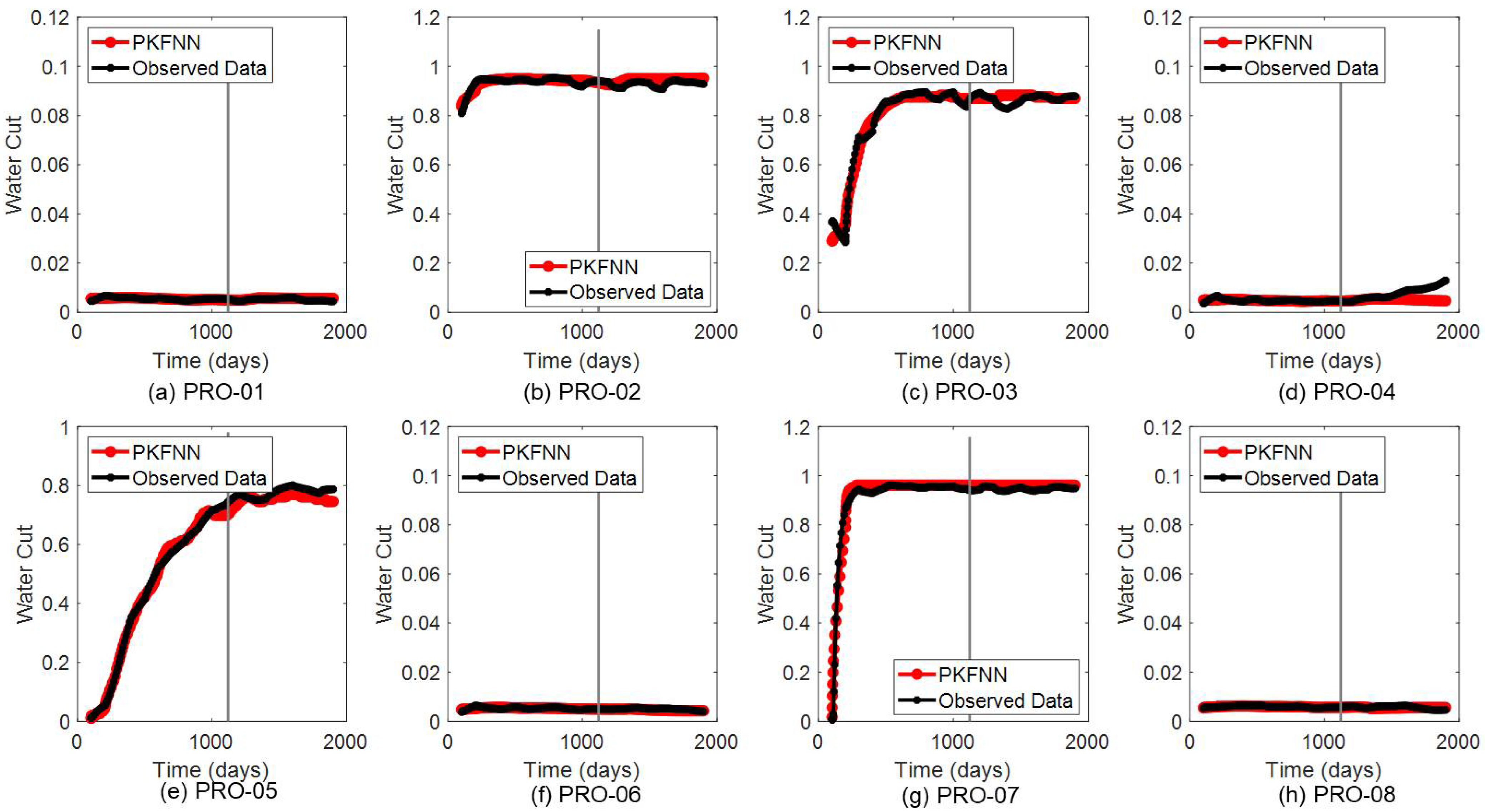
Figure 6, where the observed data is marked by the black lines, and the model outputs are denoted by the red lines. Additionally, the gray vertical lines separate the results into the history-matching stage and the productivity-forecast stage. Obviously, the proposed model can generate precise approximations for the productivity history of each producer. In terms of the productivity prediction, PKFNN can also forecast the production behaviors quite accurately for most producers; it even predicts the production future of PRO-05 with slight fluctuations. Similar to the production history-matching process, the same water-injection-rate and liquid-production-rate data are employed in PKFNN to match and forecast the water-cut curve. As illustrated in
Figure 7, the proposed model shows excellent performance on both the history-matching and future-forecasting of the water-cut data.
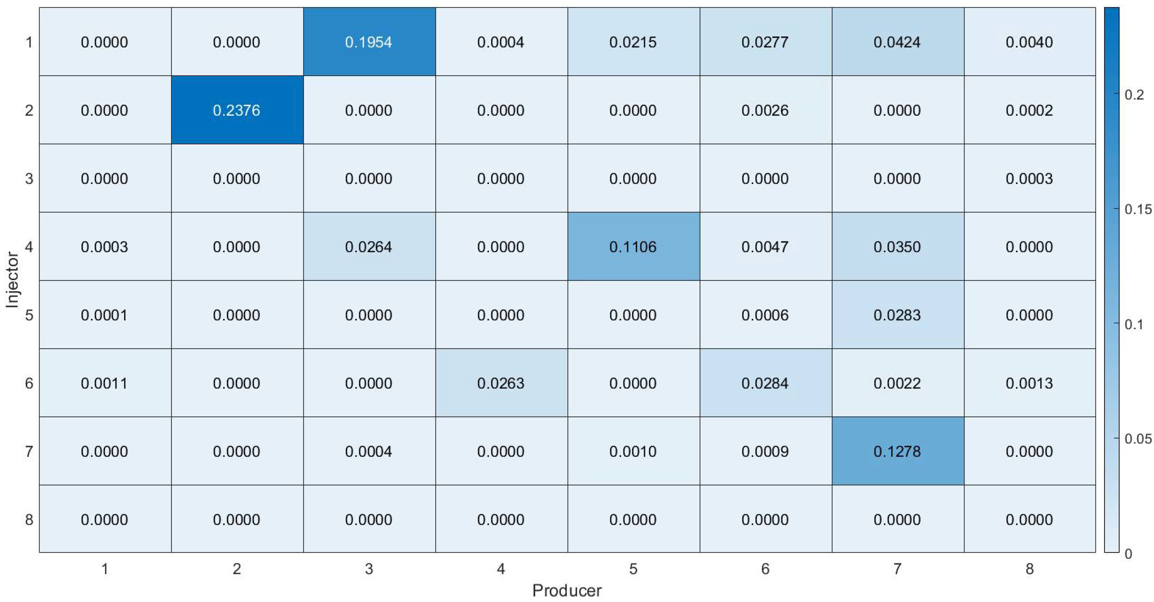
The strength of the connecting relationship between each injector and each producer is indicated by the physical evaluation function values within the knowledge-distillation block of PKFNN. With the given WIR and LPR data, PKFNN can be trained by gradient descent algorithms, and the physical function values are directly adopted as the inter-well connectivity characterization results once the training is finished. As we can see in
Figure 8, the inter-well connectivity is illustrated by the heatmap, providing a visual result for the eight-injector–eight-producer case, wherein the deeper the color, the stronger the connecting relationship between injector and producer. In contrast with
Figure 4, the four high-connecting channels, INJ-01–PRO-03, INJ-02–PRO-02, INJ-04–PRO-05, and INJ-07–PRO-07 are characterized clearly by PKFNN, which obtains 0.1954, 0.2376, 0.1106, and 0.1278, respectively. Furthermore, all the other weak-connecting well pairs are assigned to extremely low connectivity values.
To demonstrate the effectiveness of the model structure transfer learning, we compared the MSE curves obtained by PKFNN with and without model structure transfer in
Figure 9, respectively. To ensure the fairness of the comparison, we initialize the weights of the two learning models with the same normal distribution of
(0, 0.25) and take the average results by running it 10 times. As shown in
Figure 9a, all networks start with MSE values between
and
by PKFNN without model structure transfer, and these models need more than 150 iterations to converge. In contrast, as shown in
Figure 9b, except for the MSE curve of the first production well, PRO-01, (the source domain of model structure transfer), most error curves start decreasing from values that are less than
, (only the MSE of PRO-02 starts with a value between
and
).
4.2. Braided River Case
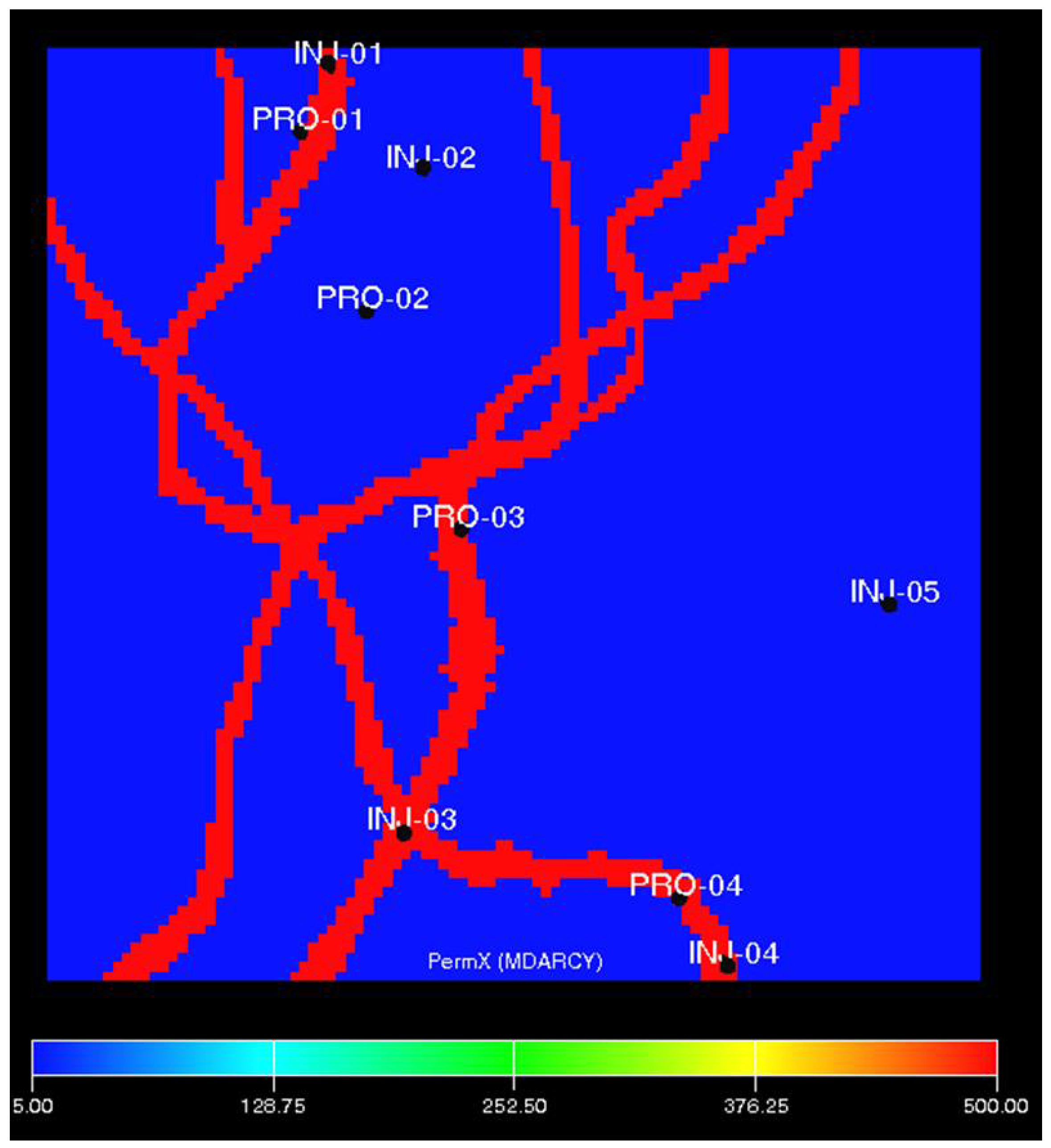
The braided river reservoir is a common fluvial deposition of the continental facies basin. As shown in
Figure 10, there are five injection wells and four production wells in this synthetic reservoir case, composed of 100 × 100 × 1 grids, and each grid is 80, 80, and 10 ft in the
X,
Y, and
Z axes, respectively. The permeability varies significantly between the channels and the matrix, with 500 md and 5 md, separately. To demonstrate the performance of PKFNN on complex production schedules, PRO-03 is converted into an injection well, and INJ-04 is converted into a production well on Day 1400. In this case, the inter-well connecting relationships would change with time. For instance, before the conversion operation, the high-connecting injector–producer pairs were INJ-01–PRO-01, INJ-03–PRO-03, and INJ-04–PRO-04, and they were INJ-01–PRO-01 and INJ-03–PRO-04 after the conversion. The simulation lasted 2600 days, and the time step was 2 days.
Table 3 lists the detailed reservoir properties, and
Figure 11 demonstrates the WIR curves of the five injectors.
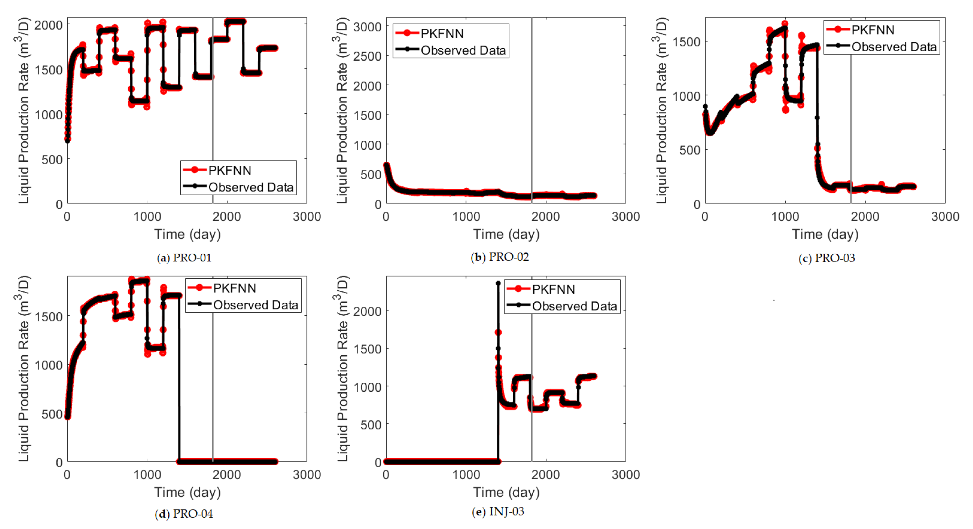
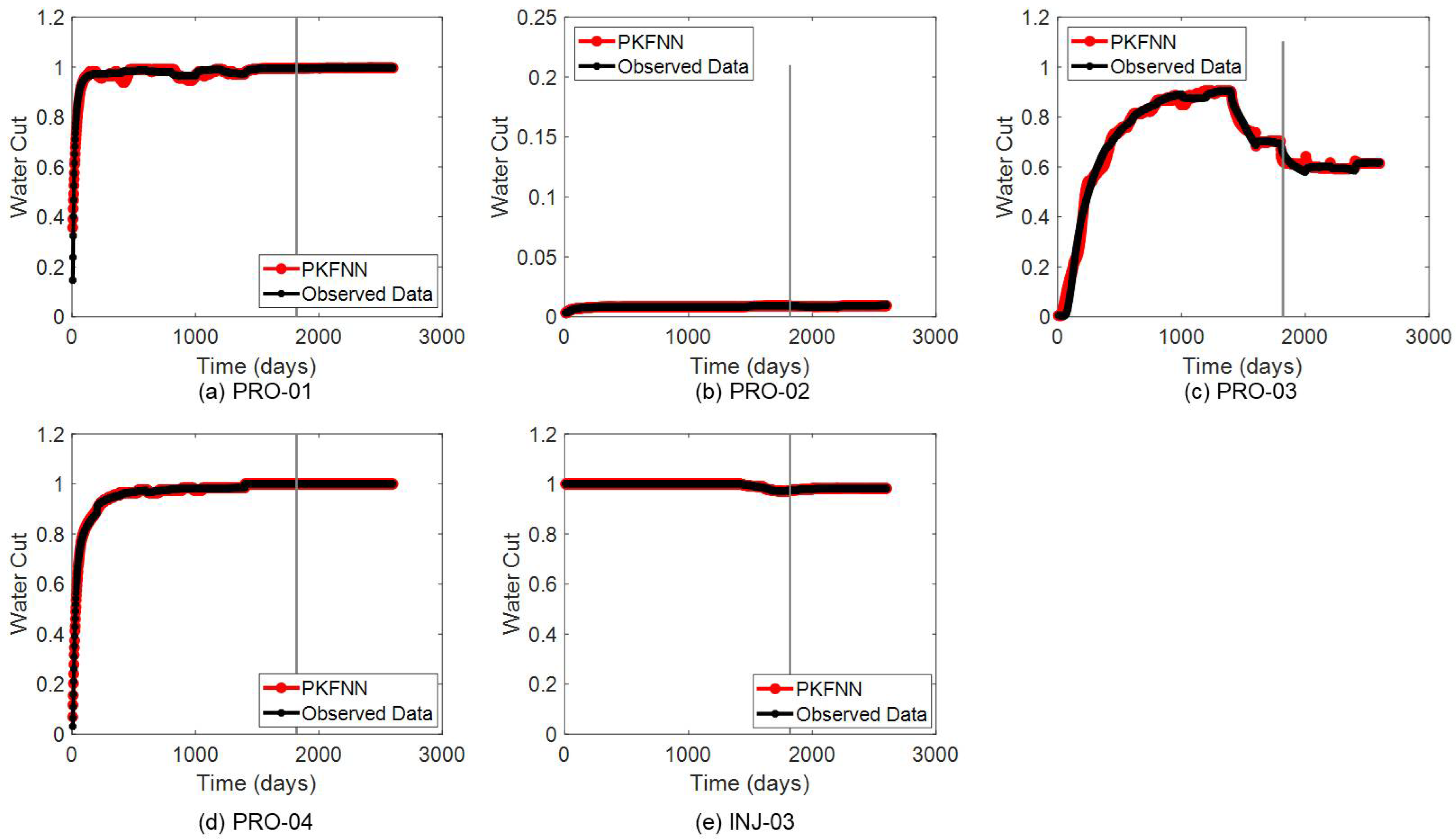
As shown in
Figure 12, PKFNN could perfectly match the productivity history and forecast the future behaviors of the five producers (including the converted production well, INJ-O3) in the braided river case. The history-matching and future-prediction results of the water-cut data are shown in
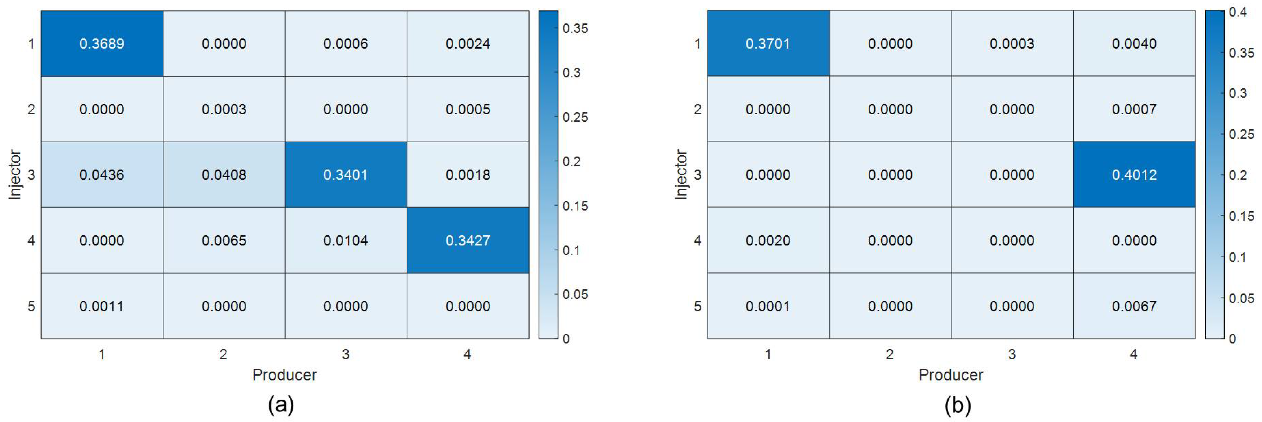
Figure 13, where PKFNN obtains quite high precision in all producers. As for the inter-well connectivity characterization, PKFNN successfully infers the strong-connecting injector–producer pairs as expected. As illustrated in
Figure 14a, the strongest-connecting injector–producer pairs before the well conversion operation, INJ-01–PRO-01, INJ-03–PRO-03, and INJ-04–PRO-04 obtain values of the evaluation function of 0.3689, 0.3401, and 0.3472, respectively. Furthermore, the other well pairs with weak connecting relationships are assigned to much smaller values than those of the three pairs, which is truly important to separate the high-flow channels from the weak-flow matrix area. In
Figure 14b, from top to bottom, the five injectors are “INJ-01, INJ-02, PRO-04, INJ-04, and INJ-05”, and from left to right, the four producers represent “PRO-01, PRO-02, PRO-03, and INJ-03”. The injector–producer pairs located on the high-permeability river channels, “INJ-01-PRO-01” and “PRO-04-INJ03”, are recognized correctly by PKFNN, which obtains values of 0.3701 and 0.4021, respectively. Furthermore, similar with the results obtained before well conversion, the weak-connecting well pairs obtain the small values in
Figure 14b.
As shown in
Figure 15, the model structure transfer effectively raises the convergence speed of PKFNN in this braided river case. For instance, as illustrated in
Figure 15a, the MSE of each producer starts to decrease from around 10
0 without transfer learning, while the initial MSE is at least lower over one order magnitude than
Figure 15a by transfer learning, as shown in
Figure 15b. In addition, PRO-02 needs less iteration times (about 50 runs) under this transfer learning frame, and the converged MSE of the other producers is also about one order magnitude lower than that without transfer learning.
4.3. Egg Case
This simulation case is designed by Zandvliet et al. [
35], including 6910 active grids, and each grid in the
X,
Y,
Z axes is 8 m, 8 m, and 4 m, respectively. There are eight injectors and four producers, injecting and producing for around 1200 days, and the other reservoir properties are shown in
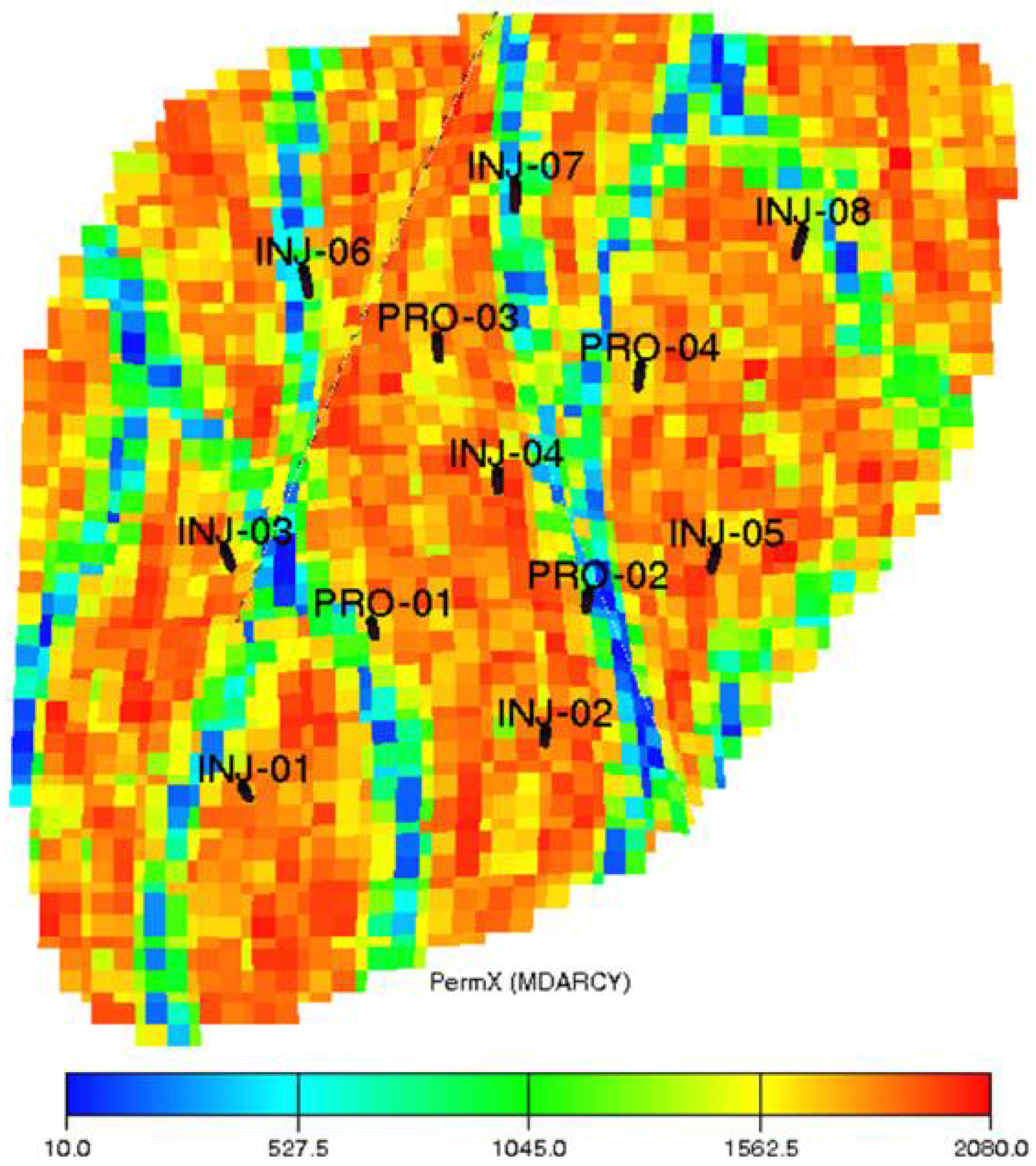
Table 4. As illustrated in
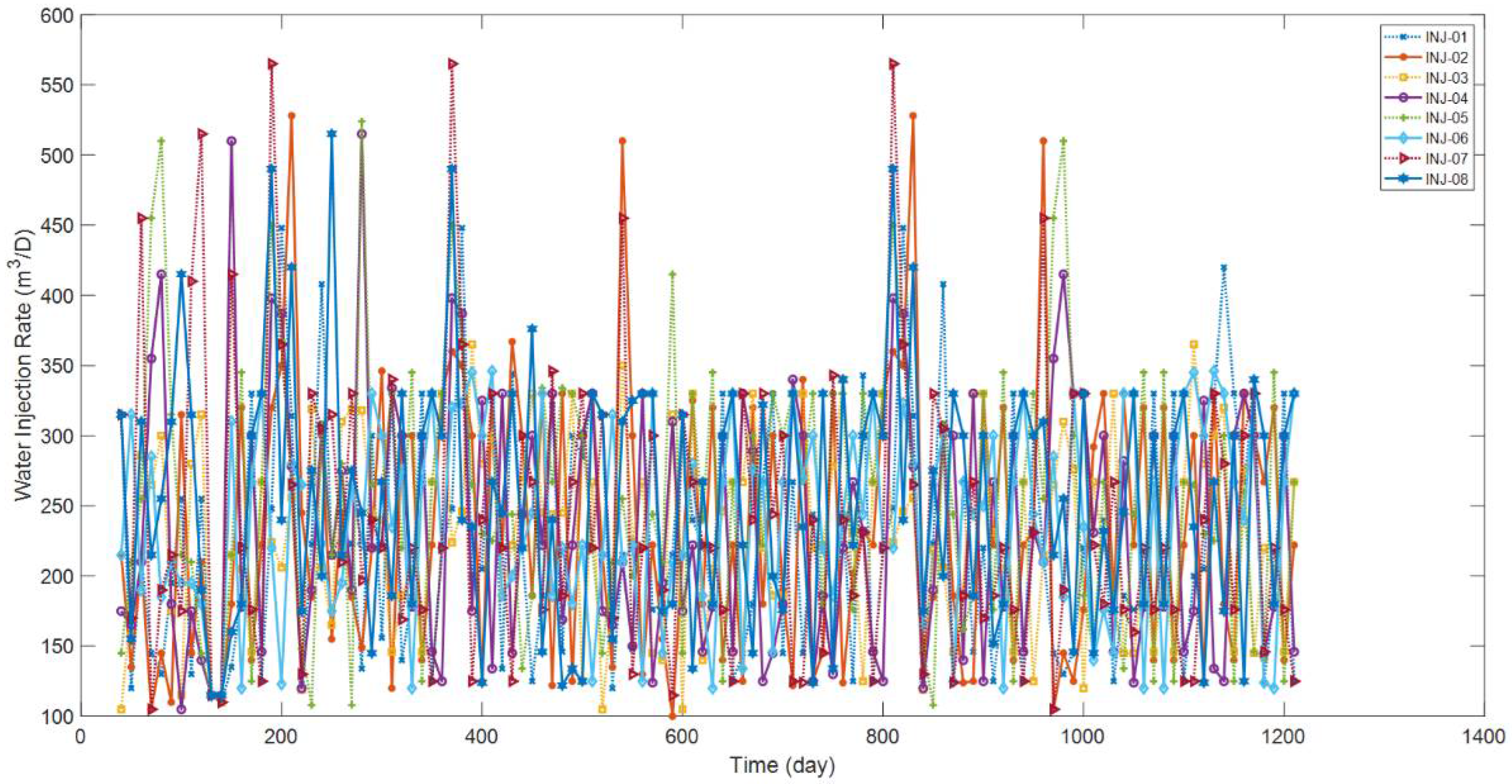
Figure 16, the permeability distribution of this experiment is very heterogeneous, which can reflect the complex geological conditions of the real reservoir to a considerable extent. The values of the permeability vary from 10 md to 2080 md, and several low permeability steaks (the blue areas) would prevent the injected fluids flow to a certain degree. In contrast, the oil stored in the high-flow areas (the red ones) is more likely to be driven by the injected water. To test the influence of the mobility ratio on PKFNN, the oil viscosity at the reference pressure (400 bar) is 10 cP. Different from the production scheme in the last two simulation cases, the injection rates change continuously and significantly with a time step of 1 day, as can be seen in
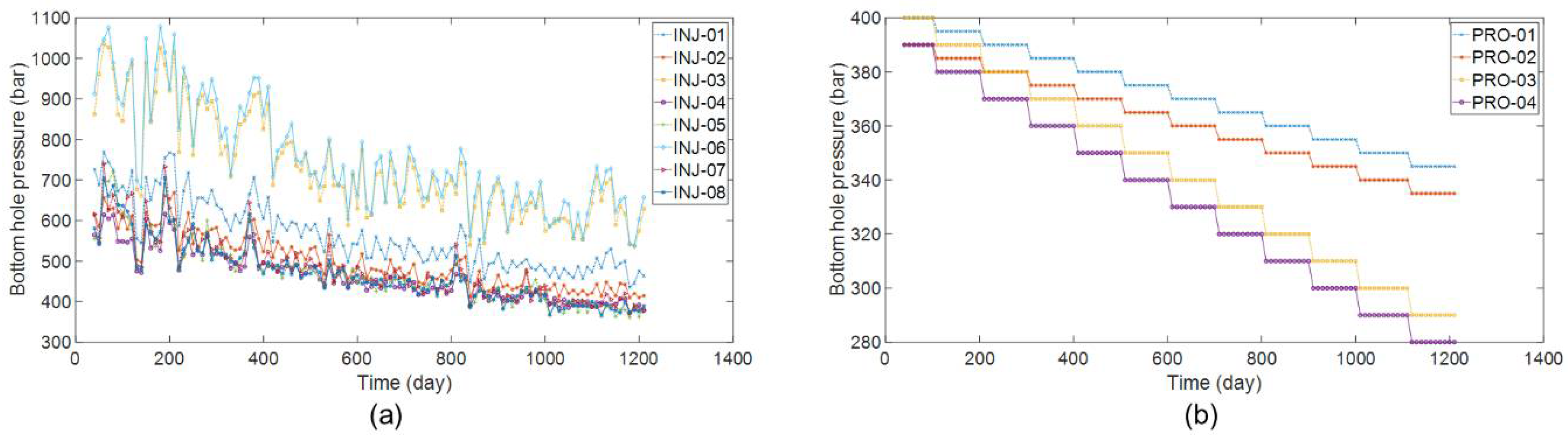
Figure 17. In addition, considering the effects of lifting pumps and structural elevations, the BHP of producers changes during the production periods. Therefore, different from the eight-injector–eight-producer case and Egg case, not only are the water injection rate and liquid production rate data used in PKFNN, but also, the variable BHP data of both injectors and producers, as shown in
Figure 18a,b, are fed to the model via the mapping-transfer block.
As can be seen in
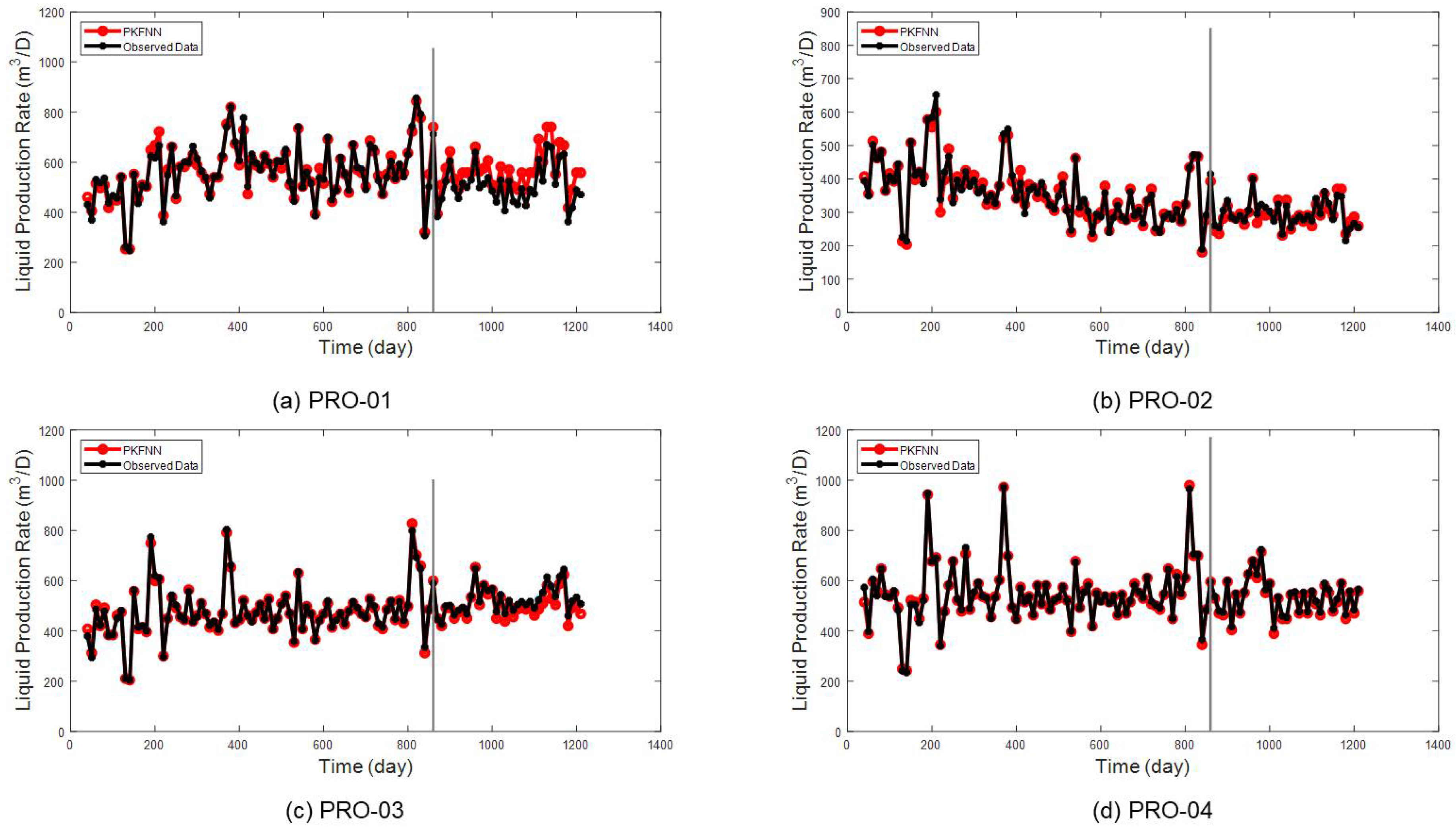
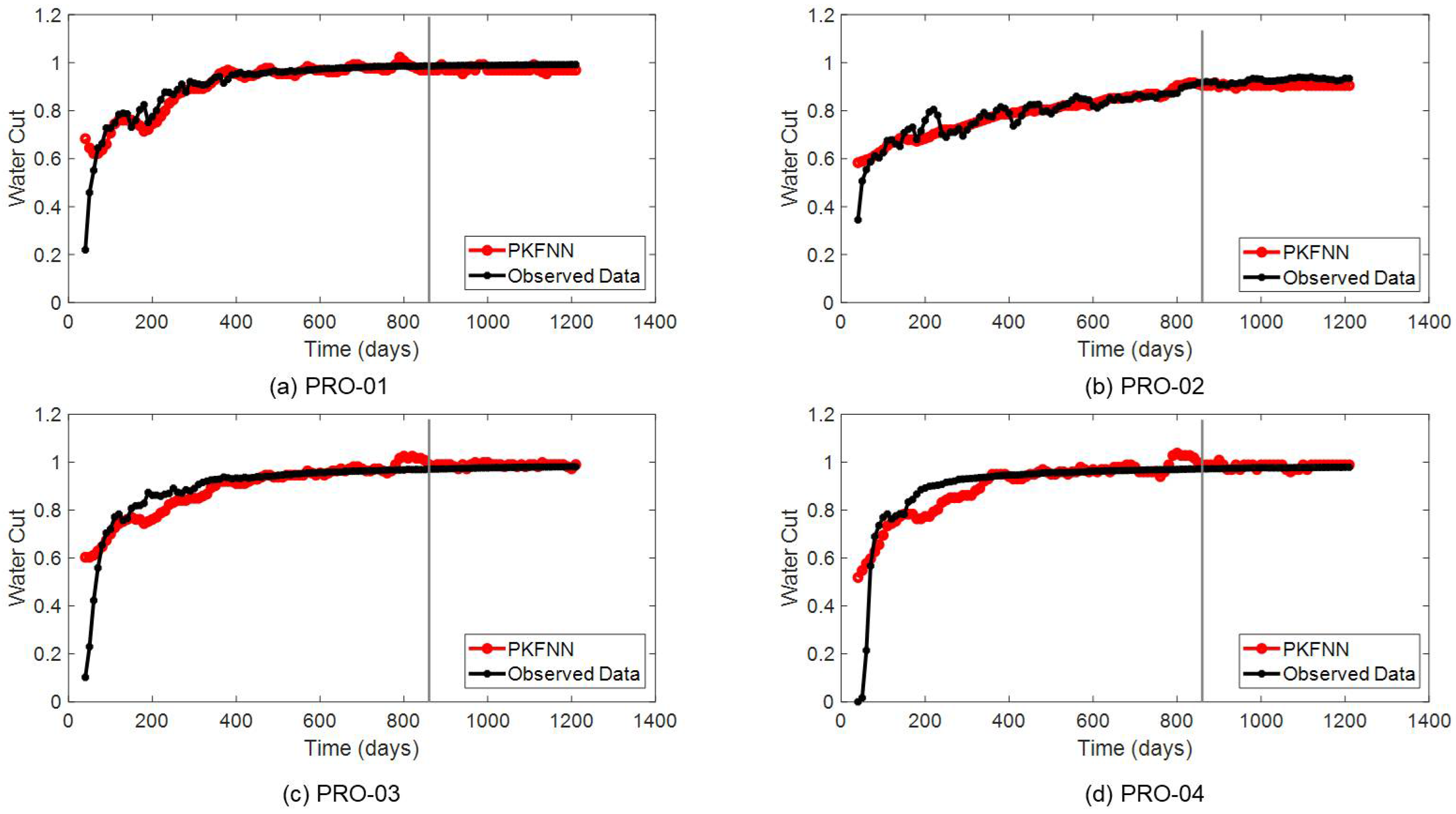
Figure 19a–d, even the productivity curves contain a lot of complex fluctuations, and the proposed model still shows a satisfying performance on the history-matching periods of all producers. As for the productivity prediction periods, PKFNN has slightly different performances on different producers. In detail, the proposed model enables the forecasting of the production future of PRO-02 and PRO-04 with quite high accuracy. However, the forecasted liquid production rates are slightly higher than the observed values for PRO-01 and slightly lower than those of PRO-O4. The history-matching and future-prediction results of water cut for four producers are shown in
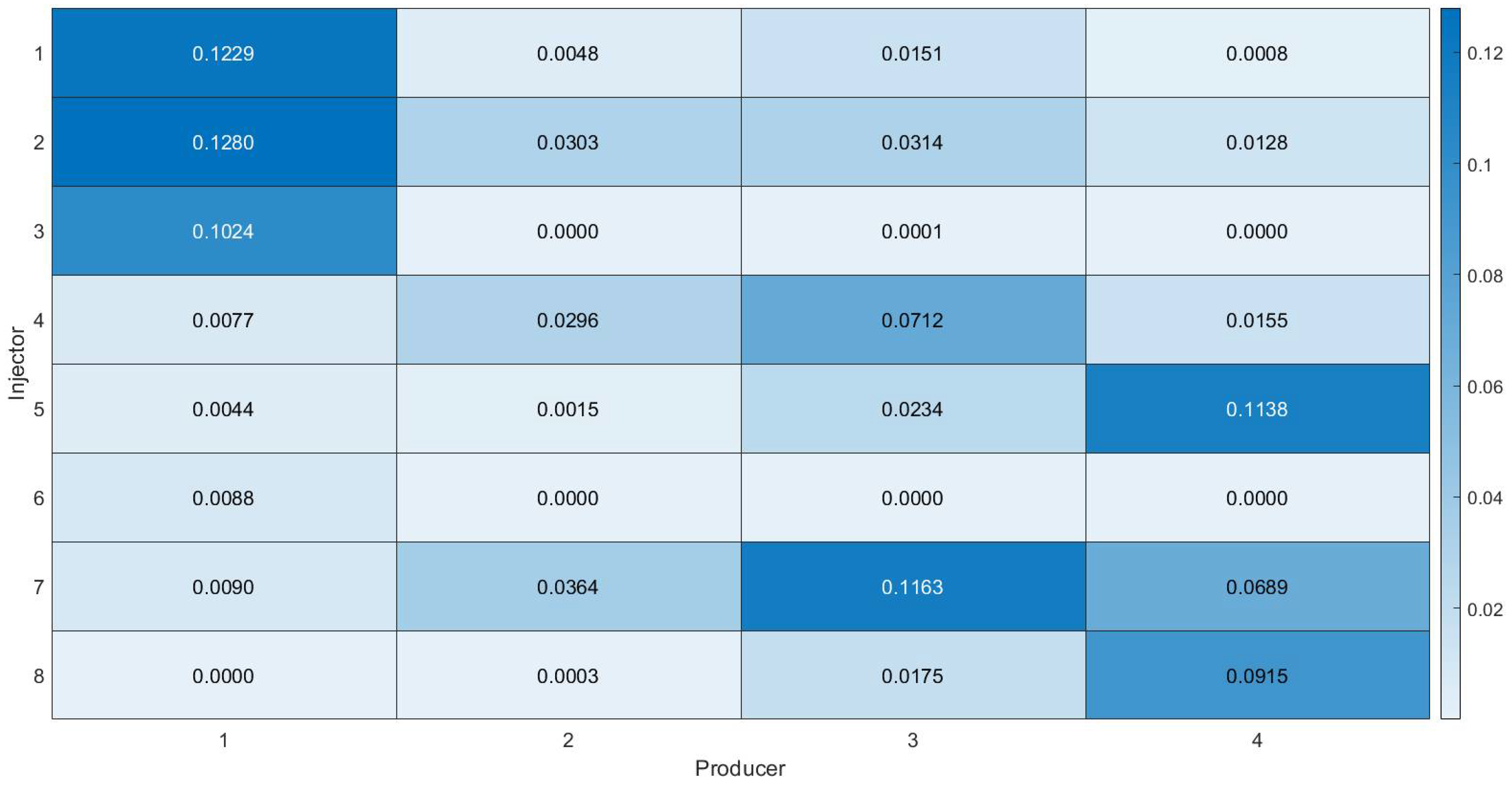
Figure 20a–d. Generally, the main trend of the water-cut curves can be matched and forecasted correctly by PKFNN, even though there are some deviations at several points between the modeled output and the observed data. For instance, at the first five points of the history-matching periods, the estimated water-cut values are higher than the observed ones in all four producers. This phenomenon might be caused by the limitation of the memory term of PKFNN, because the proposed model takes a feedforward neural network structure, which means the previous input data cannot be memorized perfectly by the model. In other words, the history input data has little effect on the model for the estimation of the current data. However, the water cut changes continuously and chronologically, so the history signals have a big influence on the estimation of the current signals. Besides, the water-cut history-matching and prediction results obtained by the proposed model may also slightly deviate from the actual values on some points. In terms of the inter-well connectivity characterization, the four injector–producer pairs located in the high permeability areas, INJ-01–PRO-01, INJ-02–PRO-01, INJ-05–PRO-04, and INJ-07–PRO-03 obtain the top four physical function values by PKFNN, 0.1229, 0.128, 0.1138, and 0.1163, respectively, as demonstrated in
Figure 21. In addition, considering the permeability and well distance, INJ-03 can make a certain contribution to the production of PRO-01, and similarly, there would be some fluids flowing in INJ-04–PRO-03, INJ-07–PRO-04, and INJ-08–PRO-04. As shown in
Figure 21, all four of these well pairs are also assigned to relatively big values by the physical evaluation function.
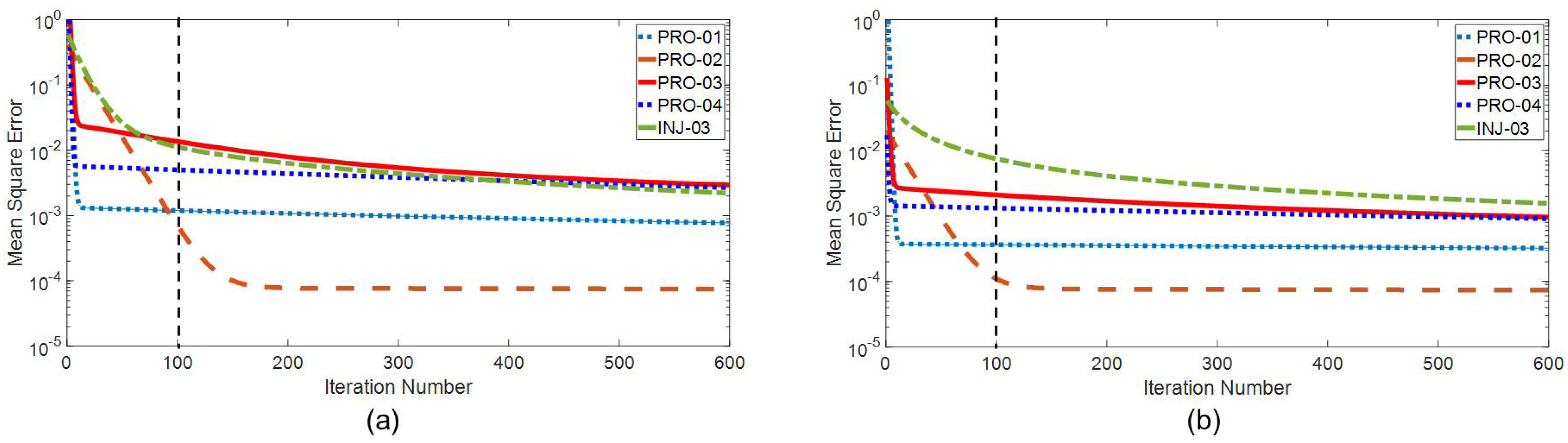
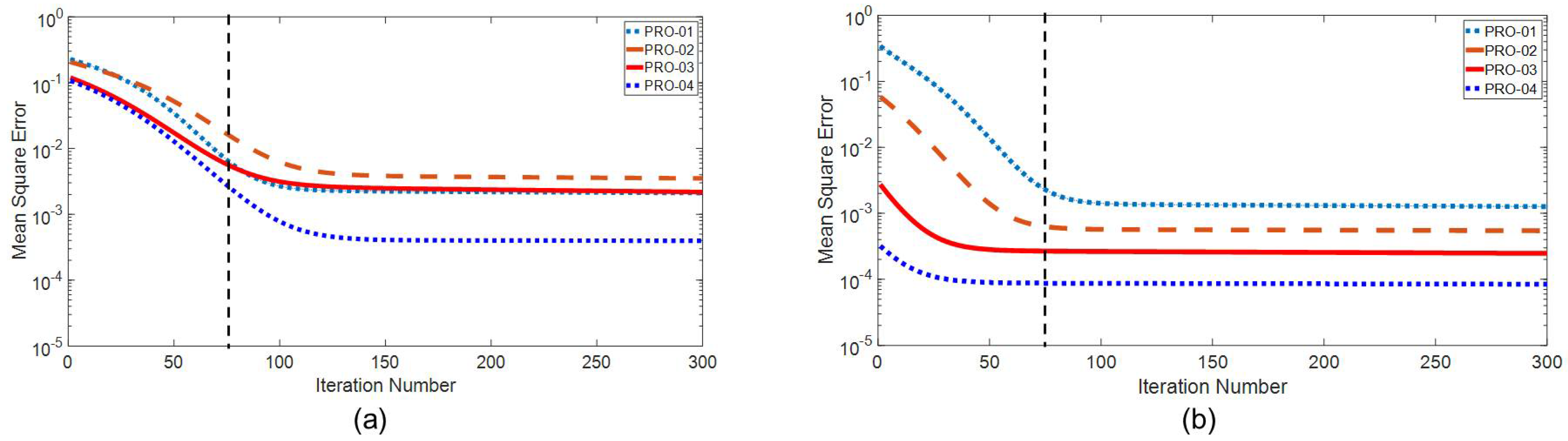
Figure 22a,b demonstrate the MSE curves of PKFNN without and with model structure transfer, respectively. On the one hand, the initial MSE values decreased by about one or two orders of magnitude by the employment of model structure transfer. In detail, all the training MSE curves of four producers start between
and
via PKFNN without structure transfer. The MSE curves in the target domain (PRO-02, PRO-03, and PRO-04) all start with values less than
. On the other hand, the convergence speed of PKFNN with structure transfer is significantly increased, and it only costs around half the iteration times (about 75 runs) of the model without structure transfer (about 150 runs).
4.4. Brugge Field Case
The synthetic Brugge reservoir model [
36] is an important representative SPE benchmark case proposed by the Dutch Organization for Applied Scientific Research (TNO), which serves as the real field in the test of history-matching and production-optimization approaches in a closed-loop workflow. The Brugge model is a typical North Sea Brent-type reservoir case, consisting of an elongated half-dome with a big internal fault, with nine layers. From the bottom to the top of the Brugge field, there are four formations with different geological properties (e.g., the porosity, permeability, and depositional environment) and thickness, named Schie, Waal, Maas, and Schelde, respectively. The permeability of the Brugge field is very heterogeneous in the horizontal direction, and it has a high-low-high sequence in the vertical direction, making the water flow from the reservoir bottom toward the top. The other geological properties are listed in
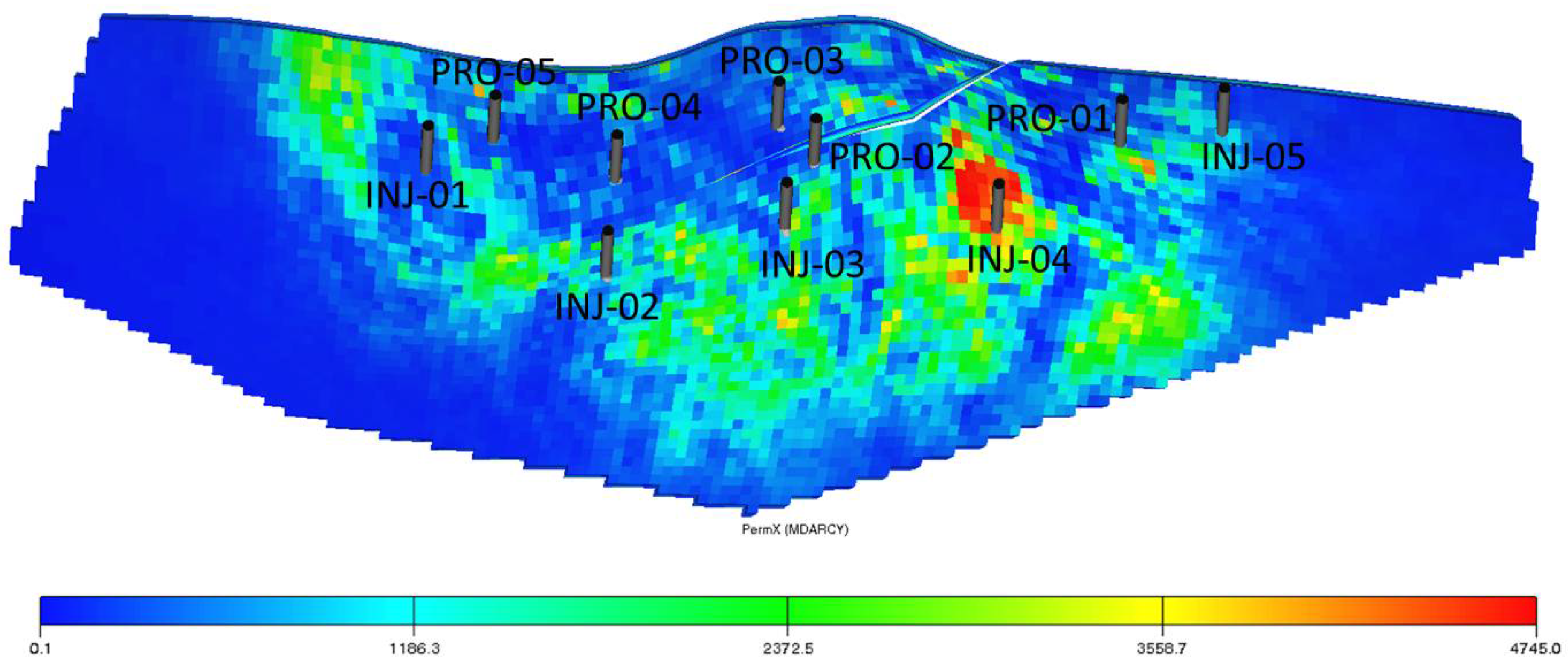
Table 5. In the primary Brugge model, there are 20 production wells and 10 injection wells, which could be controlled by 3 inflow-control valves (ICVs). In this paper, the Brugge model is simplified, retaining five injectors and five producers, as shown in
Figure 23. Besides, the original Brugge model simulates the production for 10 years, while some producers are shut in during the last 600 days. Thus, for the application of production prediction, only the data collected from the first 3000 days (which are obtained before the shut-in operation) remain for the training and testing of PKFNN.
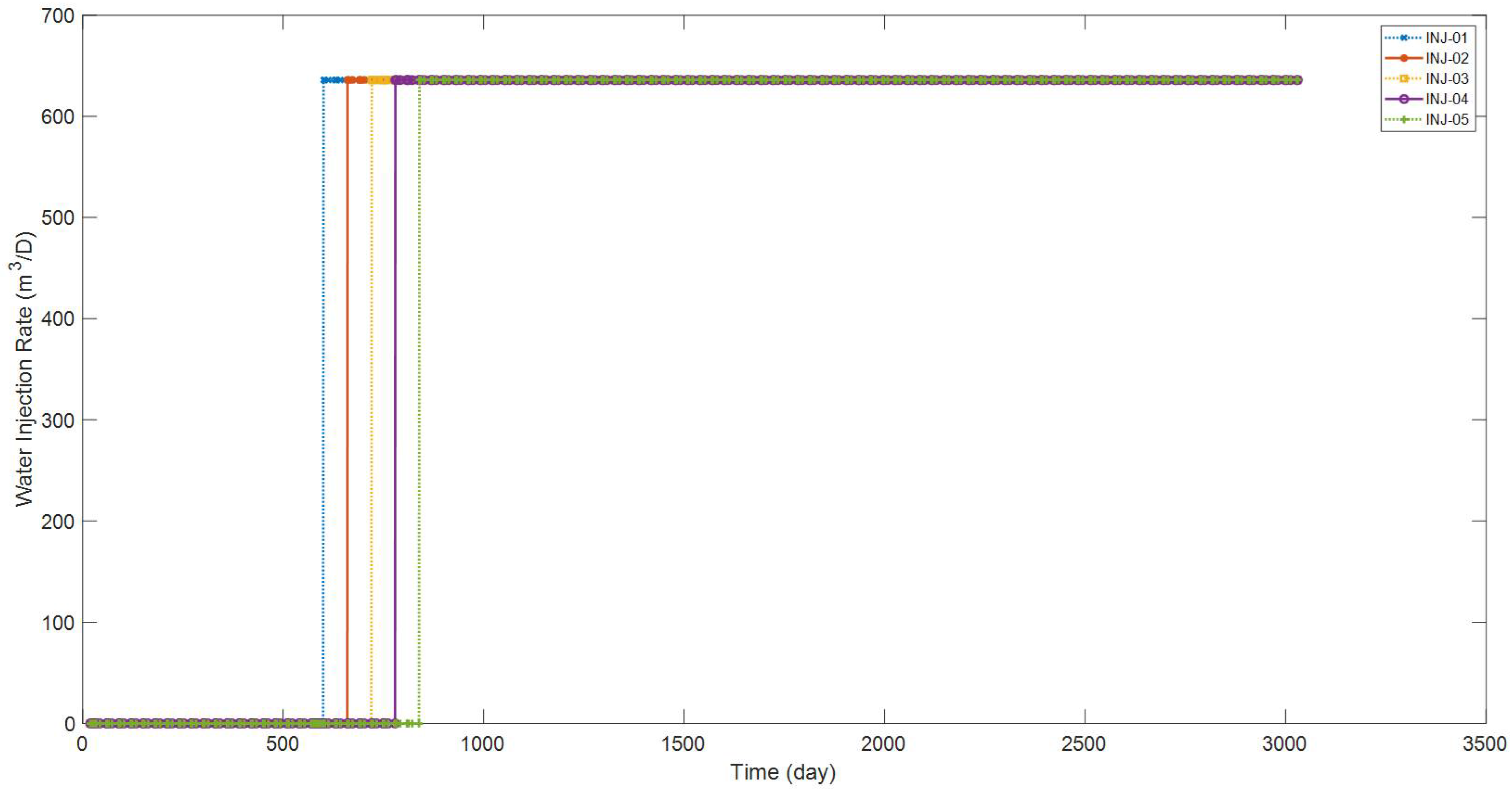
Different from the former three cases, the Brugge field case takes a much more stable water injection scheme. As shown in
Figure 24, from INJ-01 to INJ-05, the five injectors are closed at first, for 600, 660, 720, 780, and 840 days, respectively. After that, the WIR of every injector remains stable at 636 m
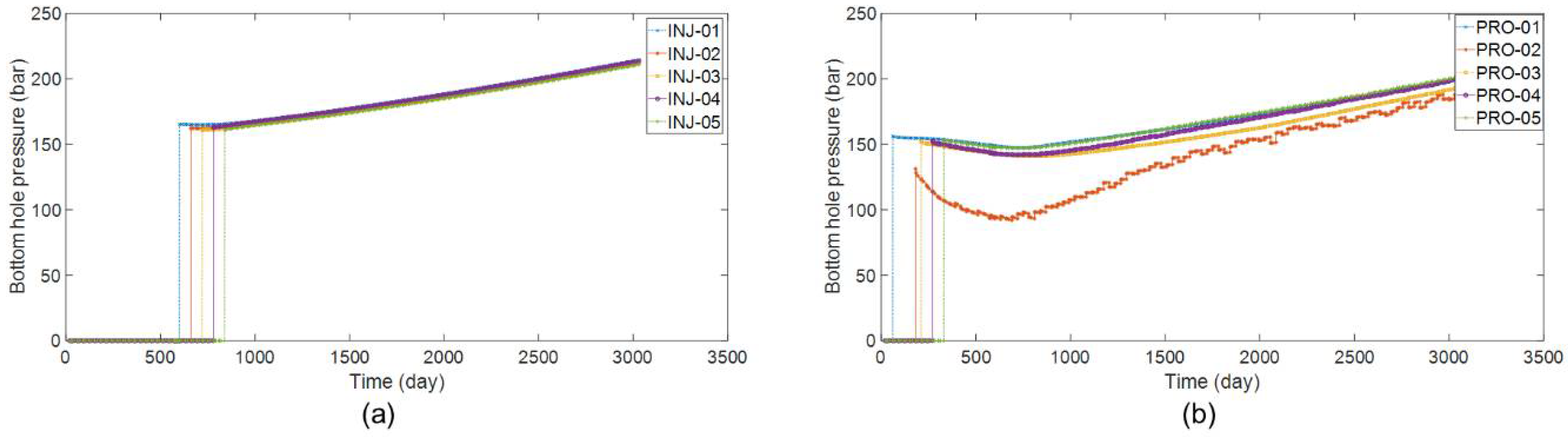
3/D until the end of production. The BHP data of the five injectors are shown in
Figure 25a, similar to the trends of the WIR curves in
Figure 24, staying at 0 bar for the same periods and growing slowly from 160 bar to 230 bar during the injection process. From PRO-01 to PRO-05, the five producers are shut in at the first 60, 180, 210, 270, 330 days, respectively, as illustrated in
Figure 25b. Then, except for PRO-02, the BHP of the other four production wells start at around 150 bar, maintain a very slight downward trend until about Day 750, and slowly increase to about 200 bar at Day 3030. PRO-02 starts production with BHP of 131 bar at Day 181, and then the BHP decreases to 92 bar at Day 690, and after that, it increases to 188 bar at Day 3030. Additionally, compared with the BHP curves of the other four producers, there are more subtle fluctuations in the BHP curve of PRO-02. Same as the training mode employed in the Egg case, in the Brugge field case, the BHP data of five injectors and five producers are also fed to PKFNN for the approximation and prediction of productivity and water cut, via the mapping-transfer block.
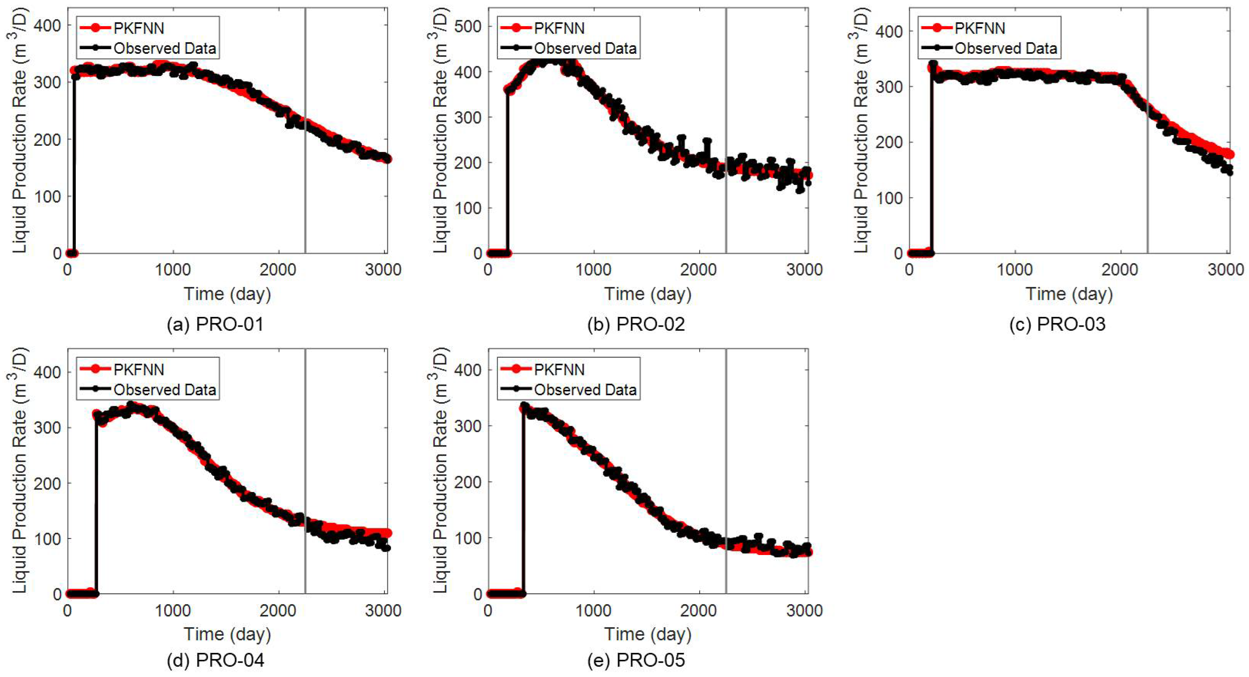
As shown in
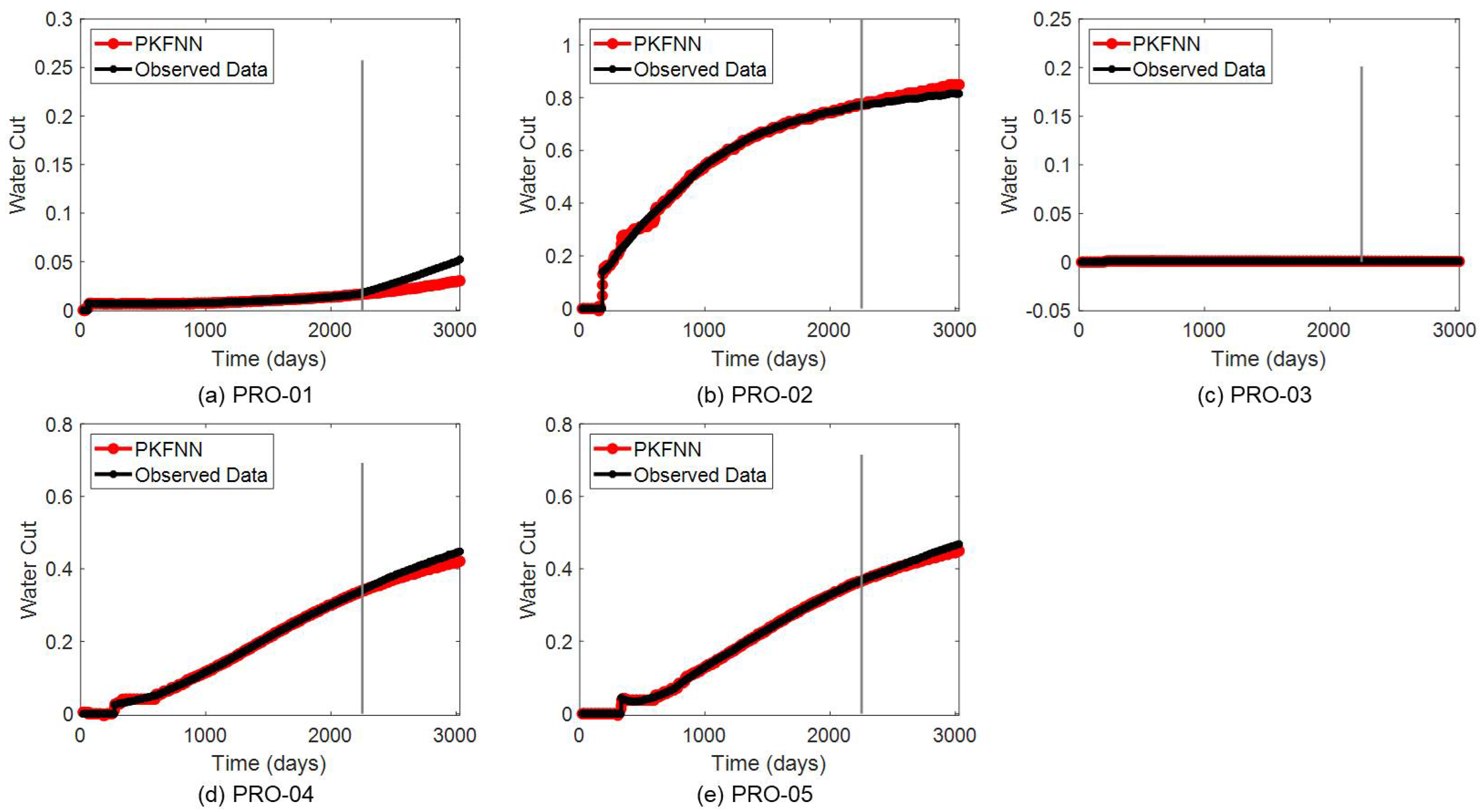
Figure 26, PKFNN still shows a great performance in the history-matching periods on five producers, and the proposed model also precisely forecasts the LPR curves of PRO-01, PRO-02, PRO-04, and PRO-05, except that the forecasted values are slightly higher than the observed ones in PRO-04. Additionally, PKFNN works well on the history-matching of water cut, as demonstrated in
Figure 27. In terms of water-cut prediction, even the forecast result of the water cut in PRO-01 slightly deviates from the true data, the average prediction error is still less than 0.03. Besides, the proposed model shows pretty good performance on the forecast of water cut for the other four production wells.
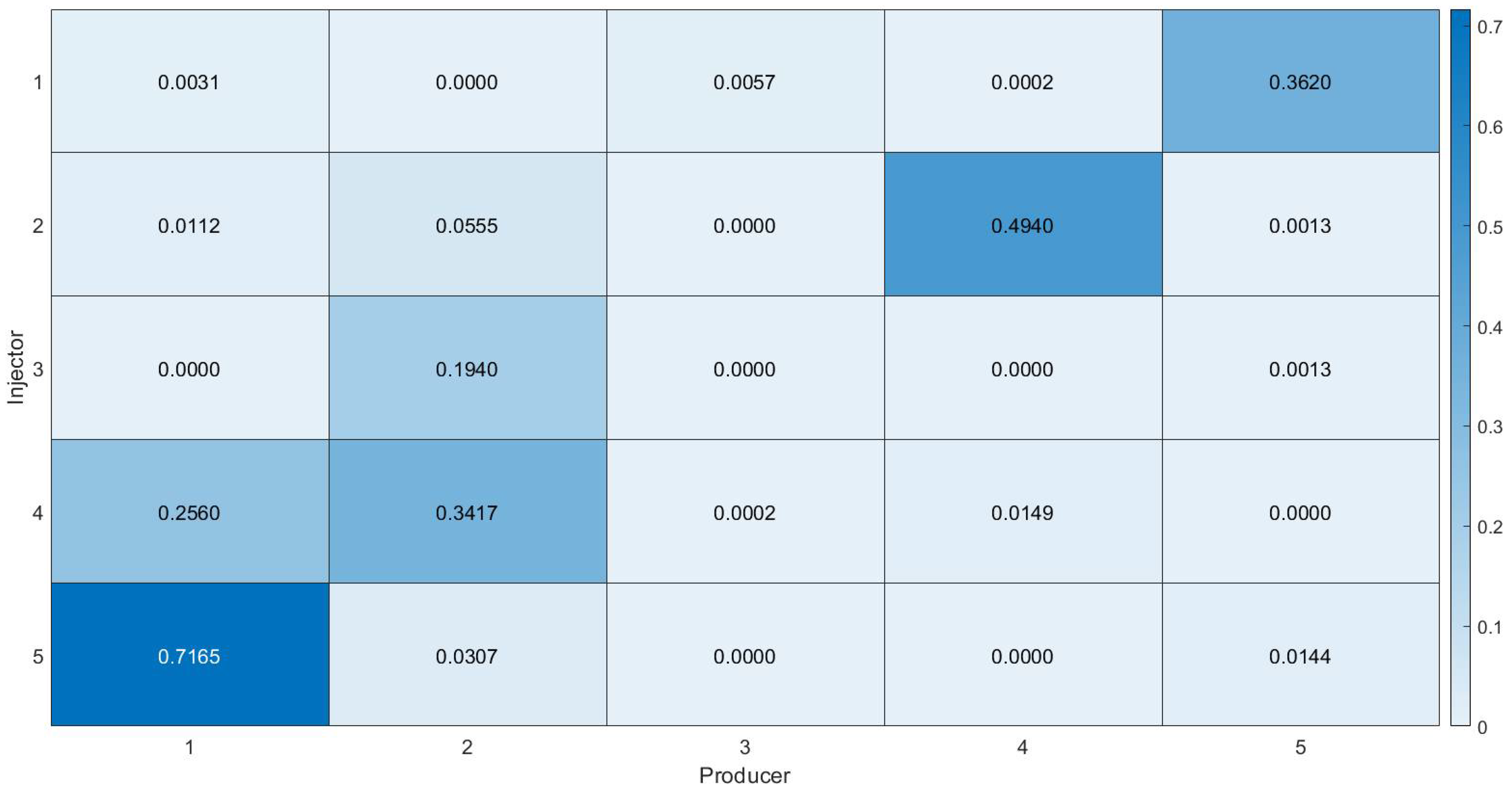
Based on the permeability field and well distance shown in
Figure 23, PRO-01 and INJ-05 are located in the high-permeability area with a close distance, and thus this injector–producer pair is expected to be recognized as the high-connecting well pair by interwell connectivity analysis. Furthermore, INJ-01–PRO-05, INJ-02–PRO-04, INJ-03–PRO-02, INJ-04–PRO-02, and INJ-04–PRO-01 should obtain relatively bigger connecting values.
The interwell connectivity characterization results given by PKFNN are demonstrated in
Figure 28, where the mentioned six well pairs are successfully inferred, with values of 0.7162, 0.362, 0.494, 0.194, 0.3417, and 0.256, respectively. Generally, the high-connecting well pairs could be reflected by PKFNN, even though there are some relative relationships between these well pairs that are not inferred perfectly. For instance, the connectivity values of INJ-03–PRO-02 (0.194) should be a little higher than that of INJ-02–PRO-04 (0.494), since the well distance of the former well pair is shorter than the latter, and the permeability around the former is also higher than that around the latter. This result might be caused by the noise of the LPR data of PRO-02, as shown in
Figure 26b.
The transfer learning mechanism still shows great performance on Brugge field case, as shown in
Figure 29. In the history matching of LPR, the model without transfer learning starts from an MSE higher than
on all producers and usually takes more than 150 iteration times to converge, as illustrated in
Figure 29a. By transferring the model structures learned from the history matching in the source domain (the task of the former producer), PKFNN could obtain an initial MSE of less than
and converge within 25 iterations, as shown in
Figure 29b.
5. Discussion and Conclusions
This paper proposes an interpretable neural network, PKFNN, to infer the connecting relationships between injectors and producers and forecast the productivity behaviors. Based on the physical knowledge of the waterflooding recovery, PKFNN associates two transparent blocks, a knowledge-distillation block and a mapping-transfer block, to approximate the underground fluids flow. In detail, the knowledge-distillation block employs a physical evaluation function to extract knowledge (the nonlinear relationships between injectors and producers). With given water-injection-rate data, this block could calculate the total inflow rate from all injectors to each targeted producer. Assisted with the ANNs, the mapping-transfer block is designed to simulate the fluid change rate of the control volume, using the BHP and liquid-production-rate data. Under the guidance of the material balance equation, PKFNN can generate the modeled production rate and water cut with the outputs of two blocks. Considering the homogeneity and continuity of the geological properties, we employ the physical knowledge transfer and model structure transfer to the parameters in the knowledge-distillation block and the mapping-transfer block, respectively, which significantly reduced the computation cost by transferring the knowledge learned from the trained models to the target domain tasks. In general, we put forward a new insight to make the ODE of the physical problem cooperate with neural networks, thereby enhancing the interpretability of model parameters and improving the generalization capability. Furthermore, considering the characteristics of the analyzed physical tasks, suitable learning techniques, like transfer learning, can be employed in the optimization to further improve the model convergence speed. We also note that there are still problems with the approximation and forecast of the data closely related to time steps, such as water cut. Thus, in the future, we would use recurrent networks, such as long short-term memory (LSTM), to tackle the industry problems.


 ,
, 


