Article

Spatial–Temporal Distribution and Interrelationship of Sulfur and Iron Compounds in Seabed Sediments: A Case Study in the Closed Section of Mikawa Bay, Japan

1
Marine Resources Research Center, Aichi Fisheries Research Institute, 2-1 Toyohama, Minami-chita, Chita 470-3412, Japan
2
Aichi Fisheries Research Institute, 97 Wakamiya, Miya, Gamagori 443-0021, Japan
3
Port and Airport Research Institute, 3-1-1 Nagase, Yokosuka 239-0826, Japan
4
Estuary Research Center, Shimane University, 1060 Nishikawatsu-cho, Matsue-shi 690-8504, Japan
5
Department of Transdisciplinary Science and Engineering, Tokyo Institute of Technology, 4259 Nagatsuta-cho, Midori-ku, Yokohama 226-8503, Japan
6
Graduate School of Environmental and Human Science, Meijo University, Shiogamaguchi, Tempaku, Nagoya 468-8502, Japan
*
Author to whom correspondence should be addressed.
Water 2023, 15(19), 3465; https://doi.org/10.3390/w15193465
Submission received: 14 September 2023 / Revised: 23 September 2023 / Accepted: 28 September 2023 / Published: 30 September 2023
(This article belongs to the Section Water Quality and Contamination)

Abstract

:
Herein, the distribution of sulfur and iron compounds (dissolved sulfide: H2S and HS, iron sulfide: FeS, and ionized iron: Fe2+ and Fe3+) in sediments (0–15 cm depth) at four stations in Mikawa Bay, Japan, was evaluated from April 2015 to March 2016. The maximum dissolved sulfide concentrations in the upper part of the sediment porewater (0–4 cm depth) (within 1.4–8.1 mmol·L−1) varied among stations located in a waterway of a large-scale port with a significant dead zone. Moreover, the iron sulfide and ionized iron concentrations in the upper part were highest at a station where the dissolved sulfide concentration was relatively low compared with that of the other sites. Analysis of the theoretical and hypothetical accumulation of particulate oxidized iron (FOOH) at the stations located in the dead zone revealed that the estimated particulate oxidized iron accumulation was higher (2303 mmol·m−2) at a station in which the dissolved sulfide concentration was low compared with the other stations (142–384 mmol·m−2). Altogether, these findings suggest that the sulfur–iron cycling can determine the amount of dissolved sulfides that accumulate in sediments. Hence, artificially adding iron compounds to the seabed may help mitigate free sulfides accumulation and prevent extreme hypoxia.

1. Introduction

For 45 years, a system for area-wide control of total pollutants load has been established to improve the water quality of the enclosed bays in Japan, including the Tokyo, Osaka, Ise, and Mikawa bays. The system has led to a steady reduction in the chemical oxygen demand, total nitrogen, and total phosphorus discharged from land areas to these enclosed bays. Nevertheless, severe hypoxia still occurs, and this has reduced the habitat availability and fishery production in Mikawa Bay during the summer [1,2,3]. Notably, excessive reduction of total nitrogen and phosphorus loads is also an important contributor to the decline in fishery resources, due to the continued decrease in their primary production [4]. Since critical hypoxic conditions are a serious environmental challenge in Japan [5], the Japanese Ministry of the Environment used bottom dissolved oxygen (DO) as an index to assess the direct influence of hypoxia on aquatic organisms.
Critical hypoxia is mainly attributed to a considerable reduction in the water purification capability provided by the tidal flat macrobenthos community, which is associated with aggressive land reclamation in Mikawa Bay [6,7]. To overcome these events, tidal flats and shallows are being restored in this area [5]. Nonetheless, intensive land reclamation has also contributed to drastically exacerbate the poor water quality in some areas. Waku et al. [8] extended the concept of the dead zone advocated by Diaz and Rosenberg [9] to coastal waters, defining dead zones as local areas where few organisms can survive due to severe environmental degradation. The dead zone associated with intensive reclamation covers an area of 27.8 km2 around the coastal waters of Mikawa Bay [8]. The upwelling of hypoxic water from the dead zone to the sublittoral zone kills the macrobenthos community and damages the general ecosystem of the bay [10]. Although large-scale ports account for a large portion (79.2%) of the dead zone, effective environmental restoration is difficult.
Extreme hypoxia is driven by dissolved sulfide derived from sulfate reduction in the seabed. Indeed, dissolved sulfide reaching the sediment surface can then escape to the water column, where it will act as an oxygen consumer, which will create anoxic conditions in the water at the bottom [11,12]. Iron is quantitatively the most important metal in many marine ecosystems [13,14], and can also contribute to the oxidation rate of hydrogen sulfide in the seawater [15,16,17]. Holmer et al. [18] reported the importance of iron oxides for the oxidation of reduced sulfides at the upper layer of the seabed in a mangrove forest. Moreover, Luther III et al. [19] suggested a dynamic seasonal cycling of sulfur and iron in salt marshes. Indeed, ferrous iron was reported to quickly react with hydrogen sulfide and sequester it as iron sulfide at iron-rich sediments in salt marshes [20]. Wijsman et al. [21] also reported that large amounts of reactive iron in the sediments of the mouth of the large river in the Black Sea can trap most of the produced sulfide in the form of iron sulfides. Using the radiotracer method, Moeslundi et al. [22] demonstrated that most iron reduction events taking place in the top 1.5 cm sediment layer are coupled with sulfide oxidation. The importance of chemical iron reduction, which traps sulfide and produces iron sulfide via sulfur and iron cycling, was reported in seawater [23,24,25,26] and freshwater [27,28] sediments. Although this mechanism can potentially prevent the accumulation of free sulfides in the sediment, only a few studies have explored the sulfur and iron cycles in dead zones, where environmental restoration is particularly necessary.
This study aimed to clarify the current state of the spatial–temporal distribution characteristics and interrelationship of sulfur and iron compounds in the dead zones of large-scale ports, where the extreme hypoxia has adversely affected the ecosystem and material circulation of the entire bay, but no effective countermeasures have been proposed so far. Year-round surveys were conducted from April 2015 to March 2016 to investigate the spatial–temporal changes in sulfur and iron compounds (dissolved sulfide, iron sulfide, and ionized iron) in the sediments. The present findings are expected to provide new knowledge on how iron compounds counteract the environmental impact of dissolved sulfides and extreme hypoxia.

2. Materials and Methods
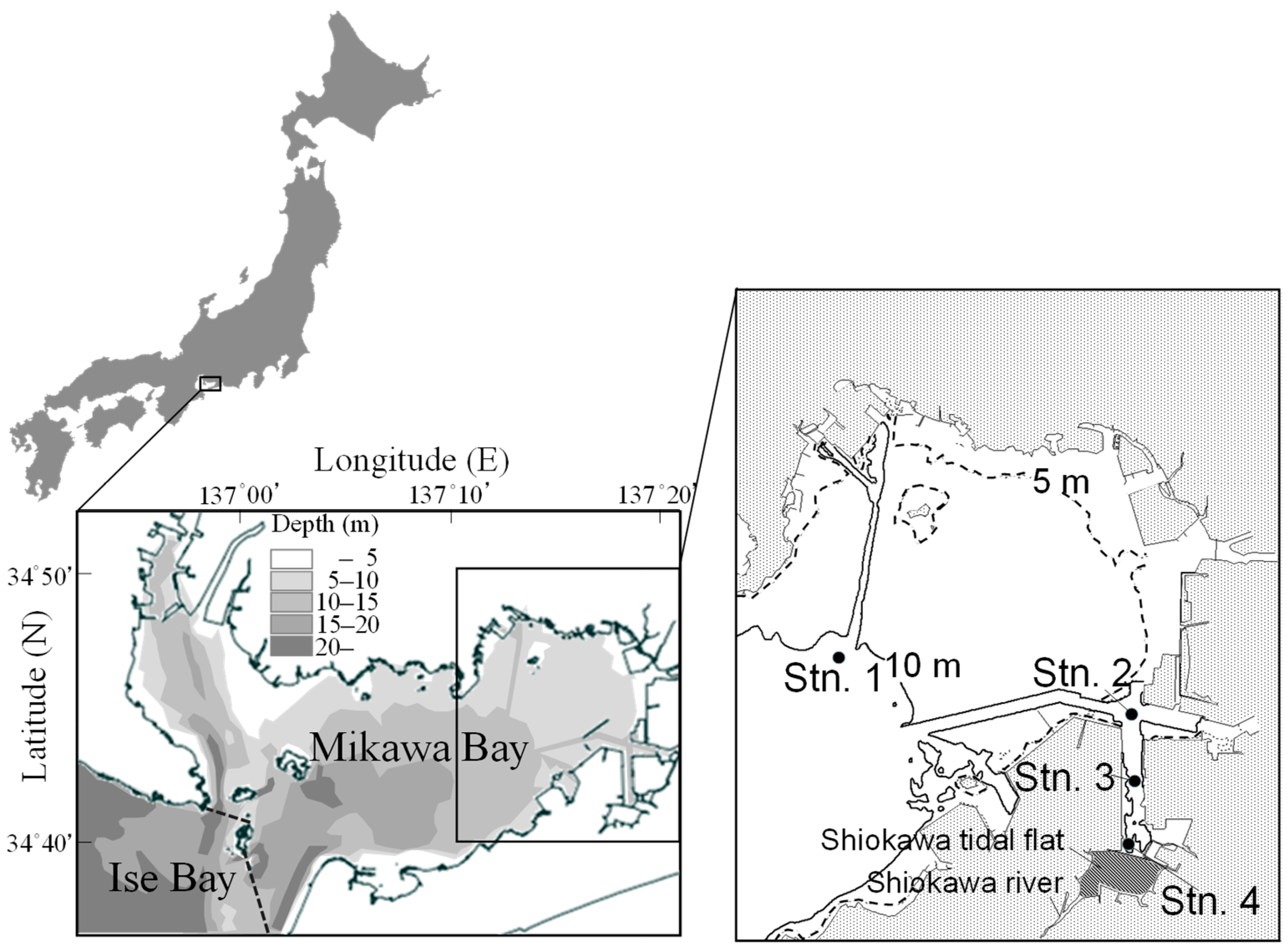
2.1. Study Site

Mikawa Bay is an embayment in central Japan that has a surface area of 604 km2 and is 9.2 m deep (Figure 1) [29]. Our survey was conducted in a closed section of Mikawa Bay, where critical hypoxia occurs annually from early summer to early autumn. The mean spring tidal range is 185 cm at the closed section of Mikawa Bay [30]. The long axis of the tide amplitude extends in an east–west direction and the tide amplitude becomes small towards the closed section of the bay. The amplitude of the springtide is a few cm·s−1 at the closed section of the bay. The residual current speed is less than 6 cm·s−1 over the year [30]. During the study period, precipitation was higher during summer compared with other seasons at Mikawa Bay. The monthly mean precipitation was 114.3 mm (88–130 mm), 299.0 mm (224–383 mm), and 91.2 mm (57–167 mm) between April and June 2015, July and September 2015, and October 2015 and March 2016, respectively, at the closed section of Mikawa Bay (Latitude 34°45.00′ N, Longitude 137°20.50′ E), according to the Japan Meteorological Agency.
Station 1 (Latitude 34°44.60′ N, Longitude 137°13.22′ E, Chart Datum Level [CDL]: −10.0 m) was located in the central part of the Mikawa Bay, and Stations 2 (34°43.82′ N, 137°18.29′ E; CDL: −11.5 m), 3 (34°42.77′ N, 137°18.30′ E; CDL: −10.1 m), and 4 (34°41.75′ N, 137°18.37′ E; CDL: −8.0 m) were located in a waterway associated with a large-scale port, which is defined as a dead zone [8].

2.2. Field Observations and Sampling

Field observations were conducted monthly at all stations from 23 April 2015, to 23 March 2016, except at station 2, which were conducted on 23 April 2015, and 27 May 2015. The tidal condition varied depending on the observation day: 23 April, 27 May, 10 August, 17 December, and 14 January were neap tide (defined as moon age 4–11, 18–26 days), whereas the other observation days were spring tide (defined as other than neap tide period).
The temperature, salinity, and DO of the water column were measured at depth intervals of 2 m from the sea surface to just above the bottom using a Conductivity-Temperature-Depth profiler coupled with a DO sensor (AAQ1182; JFE Advantech Co., Hyogo, Japan). Sediment cores and bottom water (upper 10 cm layer) were collected by scuba divers using acryl tubes (inner diameter: 4.2 cm, length: 50 cm), which were capped with rubber plugs on both ends immediately after sampling. Four sediment cores were collected at each station, and one of the samples was immediately measured for temperature, pH, and redox potential (Eh) on board using an electrical conductivity-pH meter (WM-22EP; DKK-TOA Corporation, Tokyo, Japan). The remaining sediment samples were stored in dark and cold conditions and transported to the laboratory for chemical analysis.
Additional bottom sediment (upper 4 cm depth) samples were collected at station 1 on 20 May 2015, at stations 2 and 3 on 22 June 2015, for total organic carbon (TOC) and particle size composition analysis. These samples were obtained using an Ekman-Birge bottom sampler (5141-AW; RIGO Co., Tokyo, Japan), TOC was analyzed using a MT-5 system (Yanaco Technical Science Co., Tokyo, Japan), and particle size composition was determined according to ISO 17892-4 [31].

2.3. Chemical Analysis of Sediment Samples

The top 16 cm of the sediment core was divided into eight 1 cm slices (0–1, 1–2, 2–3, 3–4, 4–5, 5–6, 9–10, 15–16 cm from the sediment surface) for chemical analysis.
The dissolved sulfide concentration in porewater was analyzed using a colorimetric method, as previously described [32], and a spectrophotometer (UV-1600; Shimadzu Corporation, Kyoto, Japan) with a 10 mm semi-micro glass cell (4 mm inside width; GL Sciences Inc., Tokyo, Japan). The detection limit was calculated to be 0.14 μmol·L−1 based on the sum of the triplicate standard deviations and the mean absorbance of the blank sample [33].
The acid volatile sulfide (AVS-S) concentration was determined using an H2S-absorbent column (201H; Gastec Corporation, Kanagawa, Japan). The iron sulfide concentration in the sediment was calculated by subtracting the dissolved sulfide concentration from the determined AVS-S concentration.
The concentration of ionized iron (Fe3+, Fe2+) in porewater was analyzed via spectrophotometric assays using 1,10-phenanthroline (ISO 6332 [34]) and a spectrophotometer (UV-1600; Shimadzu Corporation). The sliced sediment cores were placed in 50-mL tubes and the porewater was extracted by centrifugation (7930; Kubota Co., Ltd., Tokyo, Japan) at 3500 rpm for 5 min. The detection limit was calculated to be 0.08 μmol·L−1 based on the sum of the triplicate standard deviations and the mean absorbance of the blank sample [33].

3. Results

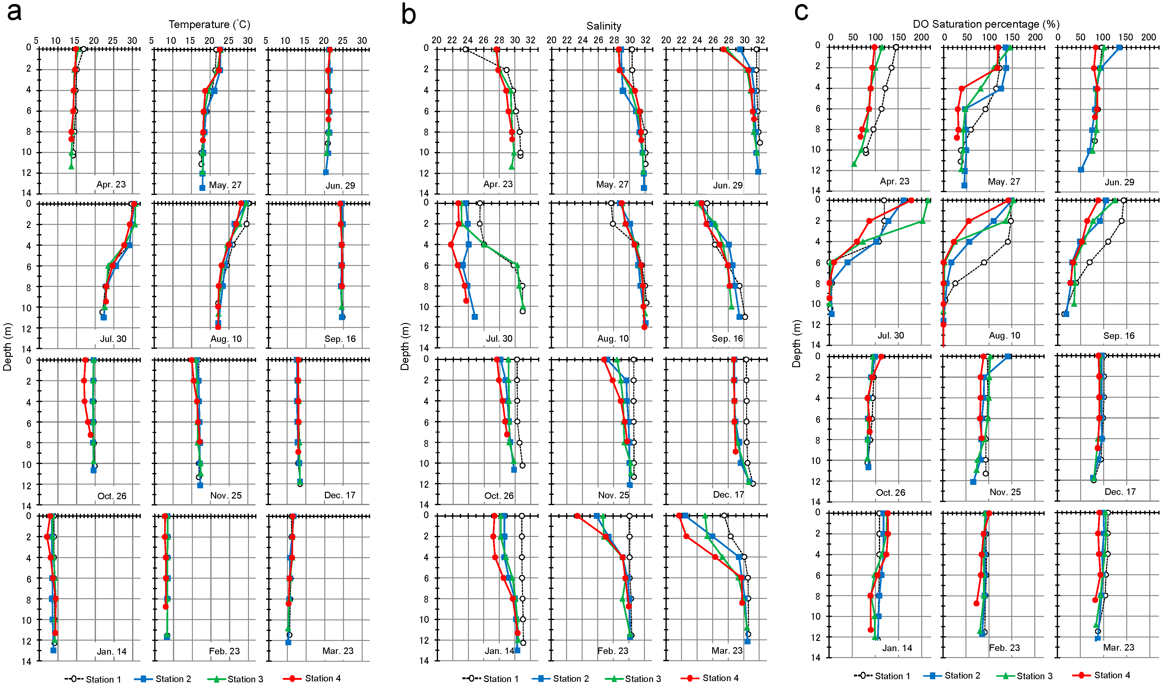
3.1. Temperature, Salinity, and Dissolved Oxygen Profiles of Seawater

Analysis of the temperature of the water column revealed a thermocline between July 30 and August 10 in all stations (Figure 2a, Table S1), with the temperature difference between the surface and bottom of approximately 7 °C, whereas the temperature was almost vertically uniform during the other months. Concerning salinity, a halocline was observed during the entire experimental period at stations 2, 3, and 4, whereas the salinity was vertically homogeneous at station 1 on 29 June, 26 October, 25 November, 17 December, 14 January, and 23 February (Figure 2b, Table S1). The surface salinity tended to be lower at station 4 than in the other stations.
Overall, the DO saturation was >30%, even in the bottom layer of each station, from 23 April to 29 June (Figure 2c, Table S1), whereas hypoxic water (<5% DO) occurred in the bottom layer, with intensive stratification in all stations on 30 July, and was maintained in all stations until 10 August. The bottom DO increased up to >14% in all stations on 16 September and DO was almost saturated throughout the water column of all stations from 26 October to 23 March. Although the tidal condition differed between 30 July (moon age 14.1 days) and 10 August (moon age 25.1 days), the seabed bottom was equally covered with hypoxic water in all stations. Moreover, although the tidal condition was also different between 25 November (moon age 13.4 days) and 17 December (moon age 5.7 days), the DO vertical profiles were similar between these two observation days. The tidal level also differed between 25 November (69 cm) and 17 December (192 cm), and between 30 July (12 cm) and 10 August (94 cm). These findings suggest that the tidal condition and level have a small impact on the DO status of the bottom water.

3.2. Total Organic Carbon Concentration and Grain Size of the Sediments

The concentrations of TOC at the upper 4 cm depth sediments ranged within 18.1–26.9 mg·g−1 dry weight in each station and was generally high in all stations (Table 1). Moreover, the grains at the upper 4 cm depth sediment were primarily very small regardless of their location, with 81.9–98.6% of the particles being <0.075 mm in diameter. Although the grain size at depths deeper than 4 cm was not measured, the particles appeared to be as fine as those in the upper 4 cm depth sediments in all stations.

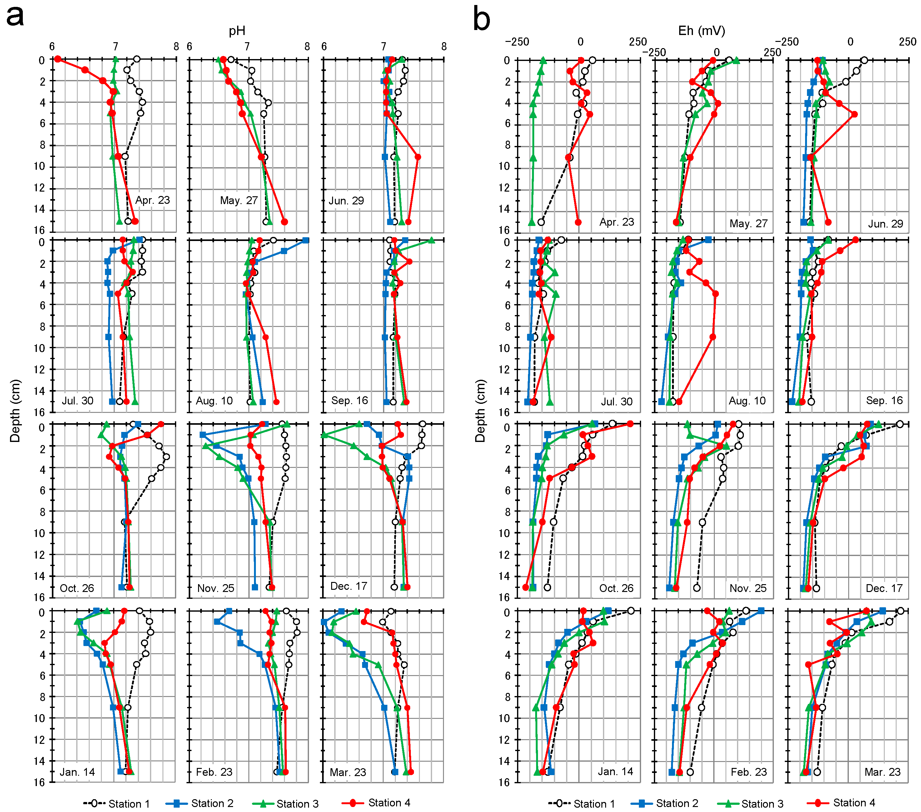
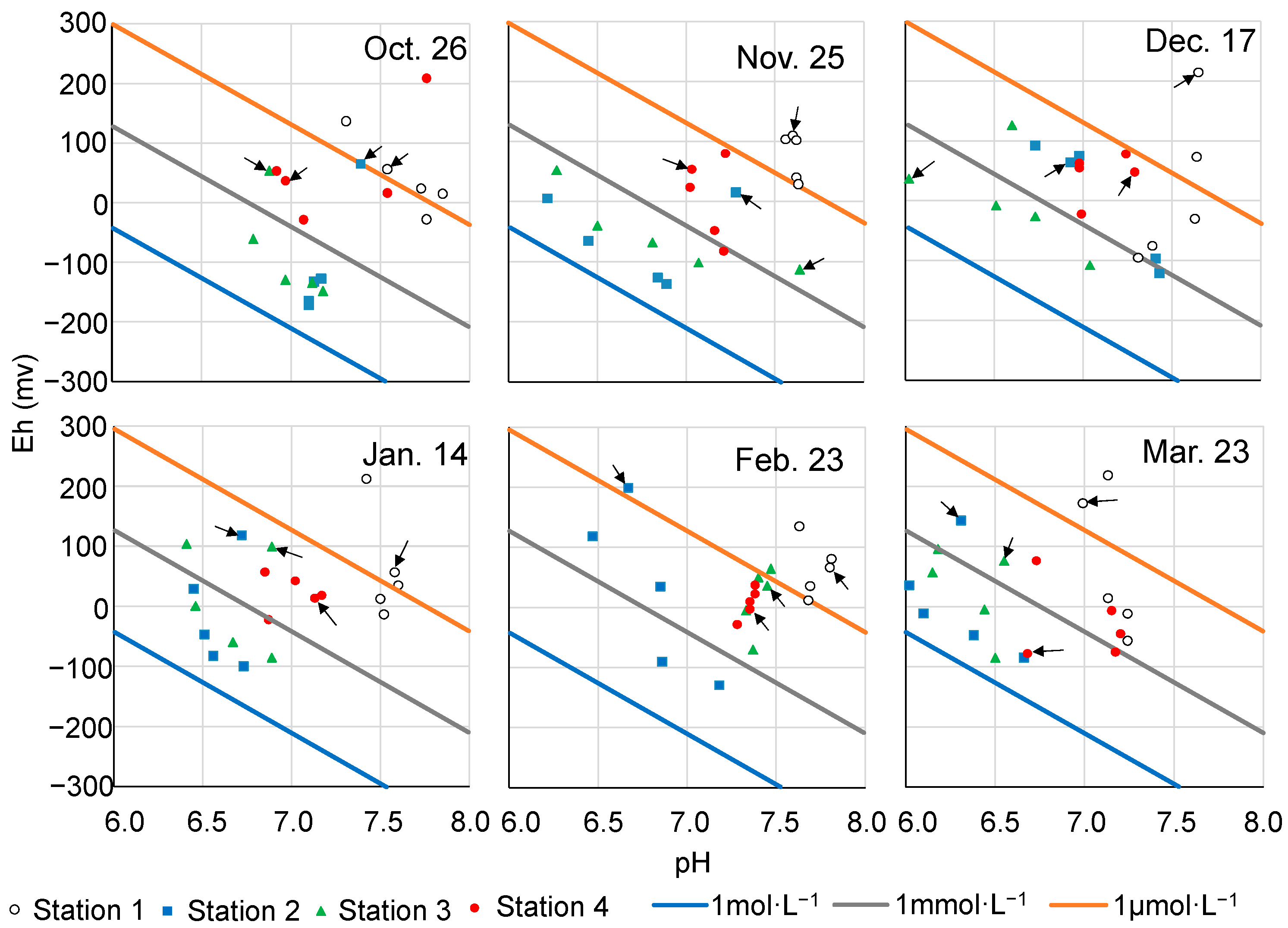
3.3. pH and Redox Potential Profiles of Sediment Porewater

The pH of the sediment porewater varied between 6.02 and 7.95 throughout the experimental period. Seasonal variations were greater in the upper 1–4 cm layer regardless of the station (Figure 3a, Table S2). The pH values >7.50 were detected in the upper 1–4 cm layer at station 1 and pH values < 6.50 were occasionally observed between 25 November and 23 March at stations 2 and 3. The lowest pH value of 6.08 was observed on 23 April at station 4. In turn, Eh was almost evenly vertically distributed at all stations in 30 July, ranging from −208 mV to as low as −71 mV (Figure 3b, Table S2). Subsequently, after 26 October, Eh increased in the upper 0–4 cm layer of each station, with positive Eh values being detected.

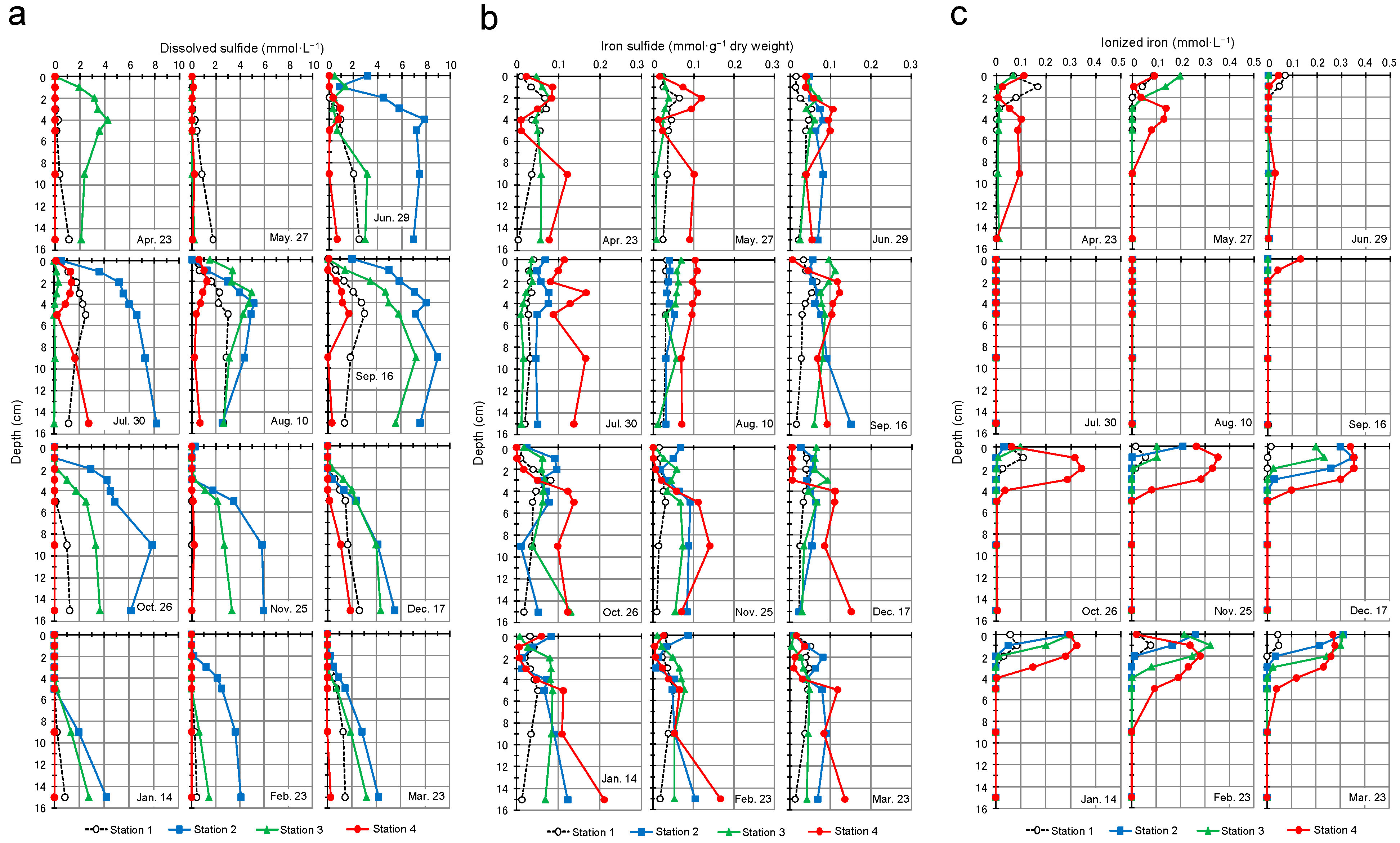
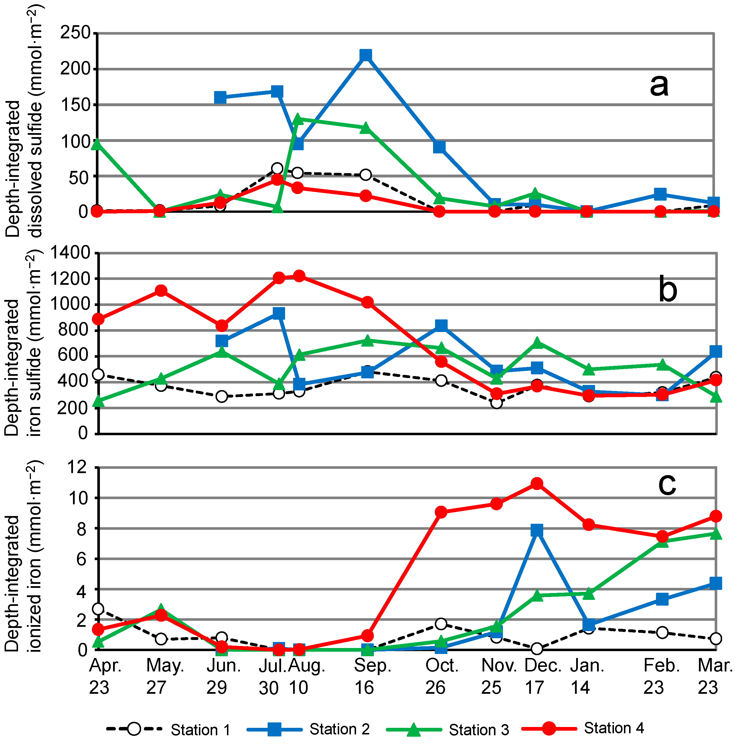
3.4. Dissolved Sulfide, Iron Sulfide, and Ionized Iron Profiles of Sediment Porewater

The highest concentrations of dissolved sulfide were detected at depths below 4 cm in all stations (3.0, 9.0, 7.2, and 2.8 mmol·L−1 at stations 1, 2, 3, and 4, respectively) during July to September, which then declined until January (Figure 4a, Table S3). The dissolved sulfide concentrations within the upper 4 cm depth layer increased at all stations within June and September, reaching a maximum concentration of 2.8, 8.1, 5.0, and 1.4 mmol·L−1 at stations 1, 2, 3, and 4, respectively. These values then decreased over time in all stations, until the dissolved sulfide was no longer detectable. Notably, the dissolved sulfide concentrations at station 4 were considerably lower than those at the other stations.
The iron sulfide concentrations tended to be low and showed less seasonal variation at station 1 compared with those at the other stations (Figure 4b, Table S4). The mean concentration of each month varied within 0.02–0.04 mmol·g−1 dry weight at station 1, and 0.04–0.08, 0.02–0.09, and 0.05–0.12 mmol·g−1 dry weight at stations 2, 3, and 4, respectively. High concentrations were detected within the upper 4 cm depth layer in the summer, and low concentrations were detected during autumn and winter at stations 2, 3, and 4. In particular, iron sulfide showed significant seasonal changes within the upper 4 cm depth layer of station 4: the maximum and minimum concentrations were of 0.17 and 0.00 mmol·g−1 dry weight on 30 July and 26 October, respectively.
Ionized iron was almost depleted throughout the sediment core from 29 June to 10 August at all stations (Figure 4c, Table S5). A small amount of ionized iron (0.04–0.13 mmol·L−1) was detected on the sediment surface of station 4 on 16 September. The ionized iron concentration increased in the upper layers of stations 2, 3, and 4 until 17 December, reaching the subsurface maximum of 0.35, 0.23, and 0.35 mmol·L−1 at stations 2, 3, and 4, respectively, and with Fe2+ accounting for 89.0–99.0% of this ionized iron. The ionized iron concentrations near the surface were maintained at relatively high values until 23 March, when Fe2+ accounted for 86.2–99.7% of this ionized iron. Conversely, ionized iron showed marginal changes throughout the year and its concentrations were substantially low. The maximum concentration detected at station 1 was 0.17 mmol·L−1 on 23 April.

4. Discussion

4.1. Seasonal Prevalence of Sulfur and Iron Compounds in Sediments of Mikawa Bay

Dissolved sulfide was distributed near the surface of the sediments during the summer, whereas DO at the bottom of the water column was depleted in the same period. Sulfate-reducing bacteria (SRB), which are ubiquitously present in lakes, river sediments, and estuaries, use organic matter and sulfate as a respiratory substrate, and dissolved sulfide (hydrogen sulfide), carbon dioxide, and water are produced through anaerobic respiration [35,36], according to the following equation:
SO42− + 2CH2O + 2H+ → H2S + 2CO2 + 2H2O.
Hence, lower bottom-water oxygen levels result in less oxidation of particulate and dissolved reduced sulfur, and resultant accumulation of more reduced sulfur [37,38]. In the present study, although the abundances of SRB were unknown, our results suggest that SRB were allowed to survive near the sediment surface (underlying anoxic bottom water), where they generally used high organic matter and sulfate, leading to the accumulation of dissolved sulfide in the sediment porewater in the summer. These findings are supported by previous studies, which described the release of dissolved sulfides from anoxic sediments into the water column [11,12,39,40]. The present study shows that part of the dissolved sulfide reaching the surface of the sediment escapes to the water column and acts as an oxygen consumer, which sustains the anoxic conditions in the bottom water.
As described above, the increase in dissolved sulfide near the surface occurred as iron sulfide increased, whereas ionized iron was depleted in the summer. Notably, Rozan et al. [41] observed a significant inverse correlation between Fe2+ and iron sulfide in the upper sediment of a shallow intercoastal bay, which resulted from Fe2+ ions that quickly reacted with hydrogen sulfide to form iron sulfide, as shown in the following equation:
H2S + Fe2+ → FeS + 2H+.
Moreover, Heijis et al. [42] attributed the overproduction of dissolved sulfide to intensive sulfate respiration accumulated in the porewater. The decrease in ionized iron observed in this study suggests that ionized iron was rapidly and effectively removed from porewaters via the precipitation of newly formed solid iron sulfide due to the presence of dissolved sulfide, as Taillefert et al. [43] reported. In addition, Fe2+ quickly reacted with the dissolved sulfide to form iron sulfide until the summer, which was followed by the depletion of Fe2+ and excess of dissolved sulfide produced by SRB accumulated in the porewater during the summer.
The increase in ionized iron near the sediment surface occurred as DO at the bottom of the water column recovered, a process that was also accompanied by a decrease in iron sulfide. These findings further suggest that Fe2+ originated from iron sulfide dissolution, which is attributed to the re-oxidation of the seabed surface with oxygen from the water column, according to the following equation:
FeS + 2O2 → Fe2+ + SO42−.

4.2. Intersite Comparison of the Sulfur–Iron Cycle

The sediment surface is important as an interface for material flux. Notably, seasonal changes in the iron and sulfur compounds were particularly noticeable in the upper layer (4 cm depth) of the sediment cores. To facilitate quantitative comparison between experimental sites with regard to the sulfur–iron cycle, we converted the measured dissolved sulfide, iron sulfide, and ionized iron contents into their density per unit of slurry volume. Figure 5 presents representative data on the seasonal changes in depth-integrated dissolved sulfide, iron sulfide, and ionized iron in the upper layer (0–4 cm depth) of the sediment core. The maximum dissolved sulfide concentrations, integrated from the surface to a depth of 4 cm of sediment in each station, ranged within 44.7–219.1 mmol·m−2 in the summer (Figure 5a). Nevertheless, the dissolved sulfide concentrations were relatively low at stations 1 and 4, located in the central bay and waterway, respectively, compared with those at stations 2 and 3, located in the waterway. Waku et al. [10] reported that the anoxic conditions of the bottom water are stable for long periods in the waterway of a large-scale port, mainly due to the reduced vertical mixing attributed to the bottom topography (which has a sharp inclination) compared with that of central Mikawa Bay. The relatively high temporal availably of oxygen supply due to vertical water mixing accounts for the relatively low concentration of dissolved sulfide at station 1 during the summer. Notably, dissolved sulfide was relatively low at station 4, despite being located on a waterway. Depth-integrated iron sulfide concentrations in the upper sediment layer of station 4 were higher (835.2–1220.6 mmol·m−2) than those in the other stations during 30 July and 16 September (Figure 5b). Moreover, the ionized iron concentration in the upper sediment layer of station 4 increased rapidly to 9.05 mmol·m−2, which was accompanied by a decrease in iron sulfide, on 26 October (Figure 5b,c). These results suggest that ionized iron was released from abundant iron sulfide; thus, more effective prevention of dissolved sulfide accumulation at station 4 is required. Nevertheless, the maximum concentration of ionized iron was 2-fold lower than that of iron sulfide at station 4.
In this study, most ionized iron was composed of Fe2+. Since the presence of Fe3+ in the sediment porewater was unlikely based on the pH and Eh at the site, it is possible that the small amount of Fe3+ detected was derived from Fe2+ oxidation during the analysis, especially during centrifugation. Therefore, in subsequent analyses, all detected ionized iron was assumed to be Fe2+.
The abundance ratio of ionized iron Fe2+ to Fe(OH)3, which is often used as a typical particulate of oxidized iron among FeOOH, is denoted by the following equation:
Fe(OH)3 + 3H+ + e = Fe2+ + 3H2O,
Moreover, the Eh related to this chemical reaction is calculated as follows:
Eh = E0 − (RT/F) × ln([Fe2+]/([H+]3 × [Fe(OH)3])) and
E0 = −ΔGF0/F,
where E0 represents the standard electrode potential (V); R is the gas constant; T is the temperature (K); F is the faraday constant; [Fe2+], [H+], and [Fe(OH)3] indicate the concentration of Fe2+, H+, and Fe(OH)3 (which is assumed to be 1) (mol·L−1); and ΔGF0 represents the total standard Gibbs energy of Fe2+ formation, which was calculated to be −93.54 × 10³ (kJ·mol−1) using each standard Gibbs energy of Fe(OH)3, Fe2+, and H2O.
Based on Equation (5), Fe(OH)3 dissolution equilibrium was further explored based on different Fe2+ concentrations (1 μmol·L−1, 1 mmol·L−1, 1 mol·L−1) (Figure 6), with Fe(OH)3 presence being more likely with higher Eh and pH values. Sediment samples from stations 2, 3, 4 with the highest levels of ionized iron were plotted between the Fe2+ dissolution equilibrium lines of 1 mmol·L−1 and 1 μmol·L−1 Fe2+. These results suggest that Fe2+ released by the oxidation of iron sulfide in the autumn (Equation (3)) was immediately converted into particulate oxidized iron. Although the concentrations of particulate oxidized iron in the experimental sites were unknown, our results suggest that it is one of the reasons for low concentrations of ionized ion compared with those of iron sulfide. Taken together, it is reasonable to speculate that Fe2+ dissolved from iron sulfide precipitates as particulate oxidized iron during the autumn and winter and that Fe2+ is re-dissolved from particulate oxidized iron during the spring and summer, thereby contributing to reduce the amount of accumulated dissolved sulfide.

4.3. Chemical Buffering Capacity toward Sulfide

Iron in sediments can potentially react with sulfide, thus preventing the accumulation of free sulfides in the sediment [13,23,24,25,26]. The capacity of the seabed to bind sulfide is known as the chemical buffering capacity toward sulfide, the sediment’s hydrogen sulfide buffering capacity, or the buffering capacity [35,43].
As mentioned previously, our finding suggests that ionized iron Fe2+ was immediately oxidized into particulate oxidized iron. Therefore, we attempted to calculate the theoretical and hypothetical accumulation of FeOOH to compare the magnitudes of buffering capacity of the sediments at stations 2, 3, and 4, which were located in a dead zone [8]. First, we calculated the theoretical and hypothetical concentration of the dissolved oxygen in the porewater that was available for FeS oxidation (Equation (3)), using temporal and spatial concentration average from the upper 4 cm sediment layer. Based on the drop in depth-integrated iron sulfide in the upper 4 cm sediment at stations 2, 3, and 4 between 30 July and 23 March (Figure 5b), the decrease rate of iron sulfide, i.e., the reaction rates (V17) [35] of Equation (3) were determined and the oxygen concentration was estimated according to the following equation:
V17 = K17 ρ (1 − φ) [FeS] [O2],
where V17 represents the mean reaction rate of Equation (3) (nmol·cm−3·s−1), K17 is the rate constant 6.0 × 10⁻⁷ (μmol·L−1·s−1) [35], [FeS] is the mean concentration of iron sulfide at 0–4 cm depth (mmol·g−1 dry weight), [O2] is the mean concentration of oxygen in the porewater (nmol·L−1), ρ is the mean density of soil particles at 0–4 cm depth (g·cm−3), and φ is the mean porosity at 0–4 cm depth (dimensionless number). Next, using the obtained O2 levels and the measured Fe2+ concentration, we determined the reaction rate (V11) [35] according to the following equations:
4Fe2+ + O2 + 6H2O → 4FeOOH + 8H+ and
V11 = K11 φ [O2] [Fe2+],
where V11 represents the mean reaction rate of Equation (8) and the accumulation of FeOOH at 0–4 cm depth (nmol·cm−3·s−1), K11 is the rate constant of 5.0 × 10⁻⁴ (μmol·L−1·s−1) [35], and [Fe2+] represents the mean concentration of ionized iron at 0–4 cm depth (mmol·L−1). Using the obtained V11 value, depth-integrated accumulation of FeOOH at 0–4 cm depth during 30 July and 23 March was calculated (Figure 7). The estimated FeOOH accumulation was higher at station 4 (2303 mmol·m−2), than that at stations 2 and 3 (384 and 142 mmol·m−2, respectively). Nevertheless, the amount of depth-integrated iron sulfide in the upper 4 cm sediments decreased at stations 2, 3, and 4 from 30 July to 23 March, up to losses of approximately 296, 98, and 790 mmol·m−2, respectively (Figure 5b). The estimated FeOOH accumulation was 1.3–2.9 times higher than the iron sulfide decrease, which can make us question the iron origin, i.e., the source of FeOOH. It is possible that rather rough calculations (especially the estimation of dissolved oxygen concentration in porewater) may have caused some deviations. However, in the present study, although the concentrations of particulate oxidized iron were unknown, it was predicted that an increase in FeOOH accumulation derived from iron sulfide oxidation at station 4, where the dissolved sulfide concentration development was inhibited. These findings further suggest that the buffering capacity can develop in dead zones through seasonal FeS–FeOOH cycling.
The Shiokawa River drains into the Shiokawa tidal flat, which is adjacent to our station 4. A large portion of ionized iron supplied from rivers coagulates and settles in the seabed, accompanied by an increase in salinity [44]. Wijsman et al. [21] reported that large amounts of reactive iron in the sediments can trap most of the produced sulfide at a river mouth. Noteworthily, the surface salinity tended to be lower at station 4 than in the other stations, which suggests that station 4 conditions were more influenced by materials from the river than the other stations. In this study, although the iron supply mechanism from the river was unknown, the buffering capacity of the sediments likely depended on the iron supply from the river. We identified the significant role played by iron pools in the prevention of sulfide accumulation in the sediment of the dead zone, where environmental restoration is particularly important.
One more important mechanism of buffering capacity is oxidation reserve, which indicates that the iron pools of the seabed can bind sulfides and therefore correspond to oxygen consumption for several months [35]. In other words, iron binds to sulfides within the sediment during the summer, causing delayed consumption of oxygen for a few months. Herein, we observed that iron sulfide precipitated by binding dissolved sulfide and rapidly ionized iron during the summer, while it was oxidized during the autumn and winter at station 4 (Figure 5). These results suggest that artificial addition of sufficient iron compounds to the seabed accelerates the chemical buffering capacity toward sulfide and prevents severe anoxic conditions in the bottom water. The iron at station 4 was considered to have originated from the nearby river, but it is also possible that accumulated iron (over years) is the main contributor to the sediment buffering capacity through seasonal cycles. Hence, artificial addition of iron for buffering capacity does not need to be a continuous process and more realistic measures to suppress sulfide generation are possible. It is believed that the attempt to suppress sulfide generation by adding iron is effective in the dead zone due to its closed and quiet characteristics. The lasting effect of reducing dissolved sulfide by adding iron-containing materials was actually previously reported in the closed section of an inner bay in Japan [45].
The maximum depth-integrated iron sulfide values of stations 2, 3, and 4 were 931.9, 722.6, and 1220.6 mmol·m−2, respectively (Figure 5b). As discussed above, on the assumption that FeS–FeOOH cycling contributes to the buffering capacity, we roughly estimated that 288.7 (1220.6 subtract 931.9) and 498.0 (1220.6 subtract 722.6) mmol·m−2 (16.1 and 27.8 g Fe·m−2) iron should be added to stations 2 and 3 to achieve equivalent buffering capacity to that of station 4, which are by no means unrealistic values. The iron sulfide concentrations were higher at lower than 4 cm depth than those at greater than 4 cm depth at stations 2 and 3; thus, the amount of iron required may be reduced by moving the FeS in the existing bottom layer nearer to the surface layer by tilling the seafloor. Nevertheless, further investigation is needed to assess the iron compound to be added by considering its availability and effectiveness, and to calculate the required amount of iron compound via quantitative analyses using numerical models.

5. Conclusions

The present study demonstrated that the amount of dissolved sulfide near the surface was higher in the summer, whereas DO was depleted at the bottom of the water column in different stations in the dead zone of Mikawa Bay. The depth-integrated dissolved sulfide in the upper layer of the sediments was relatively low at the station located near the river compared with the other stations located in the waterway associated with a large-scale port. This difference in dissolved sulfide was ascribed to the magnitude of the iron pools in the sediments, which appears to be an important factor for determining the accumulated dissolved sulfide. Moreover, the estimated particulate oxidized iron accumulation was higher at the station where dissolved sulfide concentration was low. These results suggest that artificial addition of sufficient iron compounds to the seabed may accelerate the chemical buffering capacity of the sediment toward sulfide and thus prevent severe anoxic conditions in the bottom water of dead zones.

Supplementary Materials

The following supporting information can be downloaded at: https://www.mdpi.com/article/10.3390/w15193465/s1, Table S1: Original data used to design the vertical profiles of temperature, salinity, and dissolved oxygen in the water column; Table S2: Original data used to design the vertical profiles of pH and redox potential (Eh) in the sediments; Table S3: Original data used to design the vertical profiles of dissolved sulfide speciation in the sediments; Table S4: Original data used to design the vertical profiles of iron sulfide content in the sediments; and Table S5: Original data used to design the vertical profiles of ionized iron speciation in the sediments.

Author Contributions

M.W. designed the study, measured the environmental factors, conducted the experiments, and drafted the manuscript. R.S. designed the study and measured the environmental factors. T.I. (Tetsunori Inoue) drafted and provided final approval for the manuscript. T.I. (Toshiro Ishida) measured the environmental factors. T.S. designed the study and provided final approval of the manuscript. All authors have read and agreed to the published version of the manuscript.

Funding

This research was supported by the Environment Research and Technology Development Fund of the Ministry of the Environment, Japan (no. 5-1404, Principal Investigator: Yoshiyuki Nakamura).

Data Availability Statement

No new data were created.

Acknowledgments

We wish to express our sincere gratitude to Shogo Sugahara of Shimane University for providing useful information and support. We are grateful to the crew at R/V Heiwa for their cooperation at sea. This research was jointly conducted by Aichi Fisheries Research Institute and NIPPON STEEL Corporation research teams.

Conflicts of Interest

The authors declare no conflict of interest.

References

  1. Kodama, K.; Horiguchi, T. Effects of hypoxia on benthic organisms in Tokyo Bay, Japan: A review. Mar. Pollut. Bull. 2011, 63, 215–220. [Google Scholar] [CrossRef]
  2. Sone, R.; Waku, M.; Yamada, S.; Suzuki, T.; Takabe, T. Spatio-temporal dynamics and mortality of mega-benthos in relation to the development of hypoxia in an inner bay: A model study in Mikawa Bay, Japan. Bull. Jpn. Soc. Fish. Oceanogr. 2017, 81, 230–244. [Google Scholar]
  3. Suzuki, T. Oxygen-deficient waters along the Japanese coast and their effects upon the estuarine ecosystem. J. Environ. Qual. 2001, 30, 291–302. [Google Scholar] [CrossRef]
  4. Kamohara, S.; Shiba, S.; Tsurushima, D.; Suzuku, T. Relationship of Manila clam (Ruditapes philippinarum) growth with aged changes of total nitrogen and total phosphorus in Mikawa Bay, Japan. Bull. Jpn. Soc. Fish. Oceanogr. 2021, 85, 69–78. [Google Scholar]
  5. Suzuki, T. Large-scale restoration of tidal flats and shallows to suppress the development of oxygen deficient water masses in Mikawa Bay. Bull. Fish. Res. Agen. 2004, 1, 111–121. [Google Scholar]
  6. Suzuki, T.; Matsukawa, Y. Hydrography and budget of dissolved total nitrogen and dissolved oxygen in the stratified season in Mikawa Bay, Japan. J. Oceanogr. Soc. Jpn. 1987, 43, 37–48. [Google Scholar] [CrossRef]
  7. Suzuki, T.; Ishii, K.; Imao, K.; Matsukawa, Y. Box model analysis on phytoplankton production and grazing pressure in a eutrophic estuary. J. Oceanogr. Soc. Jpn. 1987, 43, 261–275. [Google Scholar] [CrossRef]
  8. Waku, M.; Kaneko, K.; Suzuki, T.; Takabe, T. Distribution of dead zones in the coastal waters: A model study in Mikawa Bay, Japan. Bull. Jpn. Soc. Fish. Oceanogr. 2012, 76, 187–196. [Google Scholar]
  9. Diaz, R.J.; Rosenberg, R. Spreading dead zones and consequences for marine ecosystems. Science 2008, 321, 926–929. [Google Scholar] [CrossRef]
  10. Waku, M.; Hata, K.; Kaneko, K.; Suzuki, T.; Takabe, T. Adverse effects of dead zones in the coastal waters on the bay-wide material cycle and its remedial measures: An analyze with the ecosystem model in Mikawa Bay, Japan. J. Adv. Mar Sci. Tec. Soc. 2013, 19, 15–27. [Google Scholar]
  11. Brüchert, V.; Jorgensen, B.B.; Neumann, K.; Riechmann, D.; Schlosser, M.; Schulz, H. Regulation of bacterial sulphate reduction and hydrogen sulphide fluxes in the central Namibian coastal upwelling zone. Geochim. Cosmochim. Acta 2003, 67, 4505–4518. [Google Scholar] [CrossRef]
  12. Lavik, G.; Stuhrmann, T.; Brüchert, V.; Van der Plas, A.; Mohrholz, V.; Lam, P.; Mussmann, M.; Fuchs, B.M.; Amann, R.; Lass, U.; et al. Detoxification of sulphidic African shelf waters by blooming chemolithotrophs. Nature 2009, 457, 581–586. [Google Scholar] [CrossRef] [PubMed]
  13. Canfield, D.E. Reactive iron in marine sediments. Geochim. Cosmochim. Acta 1989, 53, 619–632. [Google Scholar] [CrossRef]
  14. Saager, P.M.; De Baar, H.J.W.; Burkill, P.H. Manganese and iron in Indian Ocean waters. Geochim. Cosmochim. Acta 1989, 53, 2259–2267. [Google Scholar] [CrossRef]
  15. Yao, W.; Millero, F.J. Oxidation of hydrogen sulfide by hydrous Fe(III) oxides in seawater. Mar. Chem. 1996, 52, 1–16. [Google Scholar] [CrossRef]
  16. Vazquez, F.; Zang, G.J.; Millero, F.J. Effect of metals on the oxidation of H2S in seawater. Geophys. Res. Lett. 1989, 16, 1363–1366. [Google Scholar] [CrossRef]
  17. Canfield, D.E.; Raiswell, R.; Bottrell, S.H. The reactivity of sedimentary iron minerals toward sulfide. Am. J. Sci. 1992, 292, 659–683. [Google Scholar] [CrossRef]
  18. Holmer, M.; Kristensen, E.; Banta, G.; Hansen, K.; Jensen, M.H.; Bussawarit, N. Biogeochemical cycling of sulfur and iron in sediments of a south-east Asian mangrove, Phuket Island, Thailand. Biogeochemistry 1994, 26, 145–161. [Google Scholar] [CrossRef]
  19. Luther, G.W., III; Church, T.M.; Scudlark, J.R.; Cosman, C. Inorganic and organic sulfur cycling in salt-marsh pore waters. Science 1986, 232, 746–749. [Google Scholar] [CrossRef]
  20. Antler, G.; Mills, J.V.; Hutchings, A.M.; Redeker, K.R.; Turchyn, A.V. The sedimentary carbon-sulfur-iron interplay—A lesson from east anglian salt marsh sediments. Front. Earth Sci. 2019, 7, 140. [Google Scholar] [CrossRef]
  21. Wijsman, J.W.M.; Middelburg, J.J.; Herman, P.M.J.; Böttcher, M.E.; Heip, C.H.R. Sulfur and iron speciation in surface sediments along the northwestern margin of the Black Sea. Mar. Chem. 2001, 74, 261–278. [Google Scholar] [CrossRef]
  22. Moeslundi, L.; Thamdrup, B.; Jørgensen, B.B. Sulfur and iron cycling in a coastal sediment: Radiotracer studies and seasonal dynamics. Biogeochemistry 1994, 27, 129–152. [Google Scholar] [CrossRef]
  23. Howarth, R.W. Pyrite: Its rapid formation in a salt marsh and its importance in ecosystem metabolism. Science 1979, 203, 49–51. [Google Scholar] [CrossRef] [PubMed]
  24. Howarth, R.W.; Jørgensen, B.B. Formation of 35S-labelled elemental sulfur and pyrite in coastal marine sediments (Limfjorden and Kysing Fjord, Denmark) during short-term 35SO42− reduction measurements. Geochim. Cosmochim. Acta 1984, 48, 1807–1818. [Google Scholar] [CrossRef]
  25. Drobner, E.; Huber, H.; Wächtershäuser, G.; Rose, D.; Stetter, K.O. Pyrite formation linked with hydrogen evolution under anaerobic conditions. Nature 1990, 346, 742–744. [Google Scholar] [CrossRef]
  26. Stumm, W.; Morgan, J.J. Aqueous carbonate system open to the atmosphere. In Aquatic Chemistry; Wiley-Interscience: New York, NY, USA, 1996. [Google Scholar]
  27. Wu, S.; Zhao, Y.; Chen, Y.; Dong, X.; Wang, M.; Wang, G. Sulfur cycling in freshwater sediments: A cryptic driving force of iron deposition and phosphorus mobilization. Sci. Total Environ. 2019, 657, 1294–1303. [Google Scholar] [CrossRef] [PubMed]
  28. Zhao, Y.; Wu, S.; Yu, M.; Zhang, Z.; Wang, X.; Zhang, S.; Wang, G. Seasonal iron-sulfur interactions and the stimulated phosphorus mobilization in freshwater lake sediments. Sci. Total Environ. 2021, 768, 144336. [Google Scholar] [CrossRef]
  29. Yamamoto, T.; Okai, M.; Takeshita, K.; Hashimoto, T. Characteristics of meteorological conditions in the years of intensive red tide occurrence in Mikawa Bay, Japan. Bull. Jpn. Soc. Fish. Oceanogr. 1997, 61, 114–122. [Google Scholar]
  30. Coastal Oceanography Research Committee, The Oceanographical Society of Japan. Coastal Oceanography of Japanese Islands; Tokai University Press: Tokyo, Japan, 1985. [Google Scholar]
  31. ISO 17892-4:2016; Geotechnical Investigation and Testing–Laboratory Testing of Soil—Part 4: Determination of Particle Size Distribution. Japanese Standards Association: Tokyo, Japan, 2016.
  32. Sugahara, S.; Suzuki, M.; Kamiya, H.; Yamamuro, M.; Semura, H.; Senga, Y.; Egawa, M.; Seike, Y. Colorimetric determination of sulfide in microsamples. Anal. Sci. 2016, 32, 1129–1131. [Google Scholar] [CrossRef]
  33. Kaiser, H. Zum Problem der Nachweisgrenze. Z. Anal. Chem. 1965, 209, 1–18. [Google Scholar] [CrossRef]
  34. ISO 6332:1988; Water Quality–Determination via the Iron-Spectrometric Method Using 1, 10-Phenanthroline. Japanese Standards Association: Tokyo, Japan, 1988.
  35. Fossing, H. A Model Set-Up for an Oxygen and Nutrient Flux Model for Aarhus Bay (Denmark); NERI Technical Report No. 483; National Environmental Research Institute, Ministry of the Environment: Roskilde, Denmark, 2004. [Google Scholar]
  36. Middelburg, J.J.; Levin, L.A. Coastal hypoxia and sediment biogeochemistry. Biogeosci. Discuss. 2009, 6, 1273–1293. [Google Scholar] [CrossRef]
  37. Canfield, D.E. Factors influencing organic carbon preservation in marine sediments. Chem. Geol. 1994, 114, 315–329. [Google Scholar] [CrossRef] [PubMed]
  38. Passier, H.F.; Middelburg, J.J.; de Lange, J.J.; Bottcher, M.E. Pyrite contents, microtextures, and sulphur isotopes in relation to formation of the youngest eastern Mediterranean sapropel. Geology 1997, 25, 519–522. [Google Scholar] [CrossRef]
  39. Mochida, F.; Nakamura, Y.; Inoue, T.; Higa, H.; Suzuki, T. Reproduction of the suppression effect of iron on sulfide release: Verification of the suppression effect of iron. J. Jpn. Soc. Civ. Eng. Ser. G 2021, 77, 241–250. [Google Scholar] [CrossRef] [PubMed]
  40. Inoue, T.; Hagino, Y. Effects of three iron material treatments on hydrogen sulfide release from anoxic sediments. Water Sci. Technol. 2021, 85, 305–318. [Google Scholar] [CrossRef]
  41. Rozan, T.F.; Taillefert, M.; Trouwborst, R.E.; Glazer, B.T.; Ma, S.F.; Herszage, J.; Valdes, L.M.; Price, K.S.; Luther, G.W., III. Iron-sulphur-phosphorus cycling in the sediments of a shallow coastal bay: Implications for sediment nutrient release and benthic macroalgal blooms. Limnol. Oceanogr. 2002, 47, 1346–1354. [Google Scholar] [CrossRef]
  42. Heijis, S.K.; Jonkers, H.M.; Gemerden, H.V.; Schaub, B.E.M.; Stal, L.J. The buffering capacity towards free sulphide in sediments of a coastal lagoon (Bassin d’Arcachon, France)–the relative importance of chemical and biological processes. Estuar. Coast. Shelf Sci. 1999, 49, 21–35. [Google Scholar] [CrossRef]
  43. Taillefert, M.; Bono, A.B.; Luther, G.W., III. Reactivity of freshly formed Fe(III) in synthetic solutions and (pore)waters. Voltammetric evidence of an aging process. Environ. Sci. Technol. 2000, 34, 2169–2177. [Google Scholar] [CrossRef]
  44. Boyle, E.A.; Edmond, J.M.; Sholkovitz, E.R. The mechanism of iron removal in estuaries. Geochim. Cosmochim. Acta 1977, 41, 1313–1324. [Google Scholar] [CrossRef]
  45. Miyata, Y.; Hayashi, A.; Kuwayama, M.; Yamamoto, T.; Tanishiki, K.; Urabe, N. A field experiment of sulfide reduction in silty sediment using steelmaking slag. ISIJ Int. 2014, 100, 80–86. [Google Scholar] [CrossRef]
Figure 1. Study area and location of the observation stations (stn). Solid and dotted lines represent 10 and 5 m isobaths, respectively.
Water 15 03465 g001
Figure 2. Vertical profiles of (a) temperature, (b) salinity, and (c) dissolved oxygen (DO) in the water columns at the four observation stations from 23 April 2015 to 23 March 2016.
Water 15 03465 g002
Figure 3. Vertical profiles of (a) pH and (b) redox potential (Eh) in the sediment porewater at the four observation stations from 23 April 2015 to 23 March 2016.
Water 15 03465 g003
Figure 4. Vertical profiles of (a) dissolved sulfide, (b) iron sulfide, and (c) ionized iron content in the sediments at the four observation stations from 23 April 2015 to 23 March 2016.
Water 15 03465 g004
Figure 5. Seasonal change of depth-integrated (a) dissolved sulfide, (b) iron sulfide, and (c) ionized iron in the upper 4 cm sediment layer.
Water 15 03465 g005
Figure 6. pH–Eh correlation plots according to data obtained from the upper 4 cm sediment layer of each station during 26 October and 23 March. Different colored lines indicate the Fe(OH)3 dissolution equilibrium at different Fe2+ concentrations (1 μmol·L−1, 1 mmol·L−1, 1 mol·L−1). The highest levels of ionized iron detected in each station are indicated by arrows.
Water 15 03465 g006
Figure 7. Estimated time integration of FeOOH in the upper 4 cm sediment layer.
Water 15 03465 g007
Table 1. Total organic carbon (TOC) concentration and grain size in the upper 4 cm depth sediments.
Sampling DayStationTOC
(mg·g−1 Dry Weight)
Silt and Clay Content
(Particle Diameter < 0.075 mm) (%)
20 May126.998.6
20 June222.184.9
22 June321.492.4
22 June418.181.9
Disclaimer/Publisher’s Note: The statements, opinions and data contained in all publications are solely those of the individual author(s) and contributor(s) and not of MDPI and/or the editor(s). MDPI and/or the editor(s) disclaim responsibility for any injury to people or property resulting from any ideas, methods, instructions or products referred to in the content.

