Abstract
Different regression-based machine learning techniques, including support vector machine (SVM), random forest (RF), Bagged trees algorithm (BaT), and Boosting trees algorithm (BoT) were adopted for modeling daily reference evapotranspiration (ET0) in a semi-arid region (Hemren catchment basin in Iraq). An assessment of the methods with various input combinations of climatic parameters, including solar radiation (SR), wind speed (WS), relative humidity (RH), and maximum and minimum air temperatures (Tmax and Tmin), indicated that the RF method, especially with Tmax, Tmin, Tmean, and SR inputs, provided the best accuracy in estimating daily ET0 in all stations, while the SVM had the worst accuracy. This work will help water users, developers, and decision makers in water resource planning and management to achieve sustainability.
1. Introduction
Evapotranspiration is an important factor in the hydrological cycle and is used in water resource management for irrigation [1,2], drought estimation and monitoring [3,4,5], and in estimation of crop production [6,7]. Evapotranspiration (ET) could be defined as the amount of water that is transferred from the Earth’s surface to the atmosphere, and it plays a significant role in the world’s ecosystem that is related to water, energy, and carbon cycles [8,9]. ET is affected by different factors, including precipitation, temperature, relative humidity, wind speed, and solar radiation [10]. In addition, there is a common consent that terrestrial ET around the world has been changed as a result of climate change and human activity in the last decades [11,12,13,14,15]. Therefore, in order to calculate terrestrial ET, it is necessary to recognize the roles of water management, the hydrological cycle, and the impact of climate change [16,17].
Reference evapotranspiration (ET0) can be estimated using different methods and approaches, including statistical or empirical methods, remote-sensing methods, and physical model-based methods [11]. In the first method, ET0 is estimated using flux tower observations [18,19], while in the second method, ET0 is calculated using the integration of remote-sensing data with experimental observations [20,21], the surface energy balance equation [22,23], Penman–Monteith or Priestley–Taylor equations [24,25,26], and data assimilation methods [27,28,29]. In the third method, ET0 is estimated using a physical model alone or integrated with data-simulation algorithms [30,31,32]. Although several studies have used these methods globally, the daily estimation of ET0 using these methods comes with some uncertainty [33]. Relative variation between the observed and estimated values was found to range from 14% to 44% [34,35]. On the other hand, Lysimeters provide more precise measurements of ET values, and many researchers estimate ET by employing the measurements of Lysimeters [36,37]. Unfortunately, the use of Lysimeters has some drawbacks such as the cost of installation and maintenance, in addition to environmental impacts. Additionally, the restricted number of Lysimeters impedes the observation of ET at specific locations [38]. Based on the above, the development of new adequate methods to estimate reference evapotranspiration (ET0) with more accuracy and low cost is important and necessary.
In the last decades, the use of machine learning (ML) has received more attention in the field of water resource management around the world, including ET0 estimation. ML has been applied to estimate the parameters of hydrology [39,40,41,42,43,44,45], hydraulics [46,47,48,49], and water quality by many researchers [42,50,51,52,53]. Several previous studies have reported the capability of ML techniques in estimating ET0 [54]. A comparative study using two ML techniques, namely generalized regression neural networks (GRNN) and radial basis function neural networks (RBFNN), in addition to empirical methods for ET0 estimation in Algeria, is presented in [55]. It concluded that for ET0 estimation, the results obtained from the use of GRNN are better than those obtained from using the RBF. Another ML model, which is the support vector machine (SVM) model, was developed for ET0 estimation in [56] using limited climatic data. They used different parameters such as maximum and minimum temperature, wind speed, and solar radiation with several input combinations. The results acknowledged that the SVM is useful for ET0 estimation with acceptable accuracy. A comparison between an artificial neural network (ANN) with empirical approaches to estimate ET0 using the daily meterological data has also been conducted [57]. It used two types of ANN with three empirical approaches that included Priestley–Taylor, Makkink, Hargreaves, and mass transfer. In [58], different machine learning techniques were used for ET0 estimation with more actual and precise limited meteorological variables. The results generalized the relation between the various meteorological parameters. Moreover, the performance of ten ML techniques was evaluated in [59]. It used three statistical indices that included RMSE, R2, and bias to evaluate the modeling results. In [60], a deep neural network (DNN) model was developed for ET0 estimation using four meteorological stations in Turkey. In that study, the results of DNN were compared with results of ANN. The study revealed that the output of DNN was more accurate compared to that of ANN. In [61], eight ML techniques were evaluated in estimating ET0 using temperature data only. Additionally, the results were compared with the Hargreaves–Samani equation (a temperature-based equation). It was concluded that the accuracy of the developed models varied with various scenarios. Five machine learning models to predict daily ET0 across ten meteorological stations in China were developed in [62]. The results from comparison showed that the CAT model outperformed the other models. The overall findings of the previous studies indicate that the use of soft computing techniques for modeling the evaporation process is very promising, and further studies incorporating these techniques are recommended [63].
In this research, seven scenarios with different climate variables were evaluated by employing four regression-based ML techniques. To the best of the authors’ knowledge, these regression-based ML methods have not been previously compared in estimating ET0 in a semi-arid region.
2. Materials and Methods
2.1. Study Area
The catchment area of the Diyala River is at the eastern border of Iraq towards Iran. The northern part of it (within Iran) is mostly of mountainous character, with about 3000 m height. The Hemren Basin, a large catchment area located in the northeast of Iraq within the Diyala governorate, extends between (33°53′13.00″ to 35°25′41.61″ Northern latitude) and (44°30′47.68″ to 45°48′39.59″ Eastern longitude) inside Iraqi land, and it is located about 120 km northeast of Baghdad, the capital city in Iraq (Figure 1).
Figure 1.
Location of the study area.
The relief of study area is characterized with topographic differences, their elevation ranges vary from 225 to 900 m above M.S.L. Therefore, the area was divided into three main regions. The length of the Diyala River within the catchment area is about 150 km, with an average gradient of 1 m per kilometer. Meanwhile, the Alwand River, which is the main tributary on the left side of the Diyala River, has a gradient of 2 m/km. It drains an area of 3974 km2, and without the part in Iranian land, the area is 1974 km2. The Narin River, which is the largest tributary on the right side, has a small gradient with a catchment area of 2344 km2, and empties into the Diyala River near Hemren Mountains. Moreover, the downstream part of the catchment area, located between Derbendi Khan and Hemren, has lower altitudes and gradients.
2.2. Employed Data
In the present study, the capability of four regression-based machine learning methods, SVM, RF, BoT and BaT, was investigated for ET0 estimation. Seven input scenarios were considered in this study using six climatic parameters, namely solar radiation (SR), wind speed (WS), relative humidity (RH), and maximum, mean, and minimum air temperatures (Tmax, Tmin, Tmean) as model inputs. The data were collected daily from five stations in Iraq, namely Mandali, Kalar, Iran–Iraq Border, Qarah-Tapah, and Adhim stations. Table 1 shows the statistical properties of the meteorological stations. The daily climate data during the period of 1979–2014 were collected from the study area and used for model development.
Table 1.
Details of meteorological stations used in this study.
2.3. Machine Learning Models
This section briefly explains the input combinations and machine leaning methods used in this study. ET mainly depends on temperature and other climate variables as stated by previous studies. The idea in this study was creating some scenarios including temperature as the first variable and then combining it with other variables to select which scenario was the best for predicting ET0.
Support Vector Machines (SVM) are widely recognized as powerful machine learning (ML) models that yield valuable outcomes in both classification and regression problems. The SVM methodology employs structural risk minimization during the training process, which results in several effective features for simulating complex problems [46]. These features include the sparse presentation of solutions, good generalization ability, and the ability to avoid trapping in local minima. It is worth noting that the term Support Vector Regression (SVR) is commonly used for regression-based problems.
In this method, the input vector x is transformed into a higher-dimensional space through nonlinear mapping, where linear regression is applied to the input vector. Considering a solution space with x as the independent vector and y as the dependent vector variables for the dataset having N number of data pairs, the linear regression function can be written as:
where φ(x) represents a non-linear function that maps the low input space to the high output space; w represents the weights vector, while b denotes the threshold.
Unlike the SVR model, the other three ML models, RF, BaT, and BoT, are based on the concepts of decision and regression tree models that employ ensemble learning techniques. Decision tree learning is a supervised learning approach that is used to solve both classification and regression problems. Examples include Classification and Regression Tree (CART) models. In a decision tree model such as CART, each decision node in the tree represents a test on some input variables. Ensemble learning is a prosperous ML paradigm that merges a group of learners, rather than relying on a solitary learner, to forecast unfamiliar target attributes. It has been proven that using ensemble learning can improve the simulating and predicting results of individual models [64]. In this respect, two types of ensemble learning methodologies, namely bagging (here for the Bat and RF models) and boosting (here for the BoT model), are applied.
As indicated by [65], the BoT model incorporates important advantages of tree-based methods and has unique features. Its performance is based on an ensemble for training new samples. On the other hand, the bagging technique, also known as bootstrap aggregated, is an early ensemble method, which has numerous trees designed to improve the stability and accuracy of models. In the BaT, multiple independent decision trees can be constructed simultaneously on different segments of the training samples by utilizing distinct subsets of accessible characteristics.
Random forests are one of the most popular machine learning algorithms. They are so successful because they provide in general good predictive performance, low over-fitting, and easy interpretability. This interpretability is given by the fact that it is straightforward to derive the importance of each variable on tree decision. In other words, it is easy to compute how much each variable is contributing to the decision. The RF model acts similar to the BaT by constructing different decision trees. However, it uses a classification methodology for combining multiple trees to arrive at a conclusive outcome using the voting technique. Consequently, the RF classifier exhibits a robust ability to generalize. The RF can be considered as a specified type of the Bootstrap model. In each stage, the system has two subdivisions as unconnected segments to reduce the mean squared error values.
Feature selection through the random forest (RF) is categorized as an embedded method. Embedded methods encompass the advantages of both filter and wrapper techniques, as they rely on algorithms with built-in feature selection capabilities. Embedded methods offer several advantages, including:
High accuracy: They yield precise results.
Improved generalization: They enhance the model’s ability to apply learned patterns to new data.
Interpretability: They provide insights into the significance of selected features.
Random forest comprises multiple decision trees, each constructed using a random subset of observations and a random subset of features from the dataset. This means that not every tree processes all the features or observations. This design ensures that the trees are uncorrelated, reducing the risk of overfitting. Each tree is essentially a sequence of binary questions based on individual or combined features. At each node (corresponding to each question), the tree partitions the dataset into two groups, each containing observations that are more similar to each other and dissimilar to those in the other group. Consequently, the importance of each feature is determined by how “pure” each of these partitioned groups becomes.
2.4. Evaluation of Models’ Performance
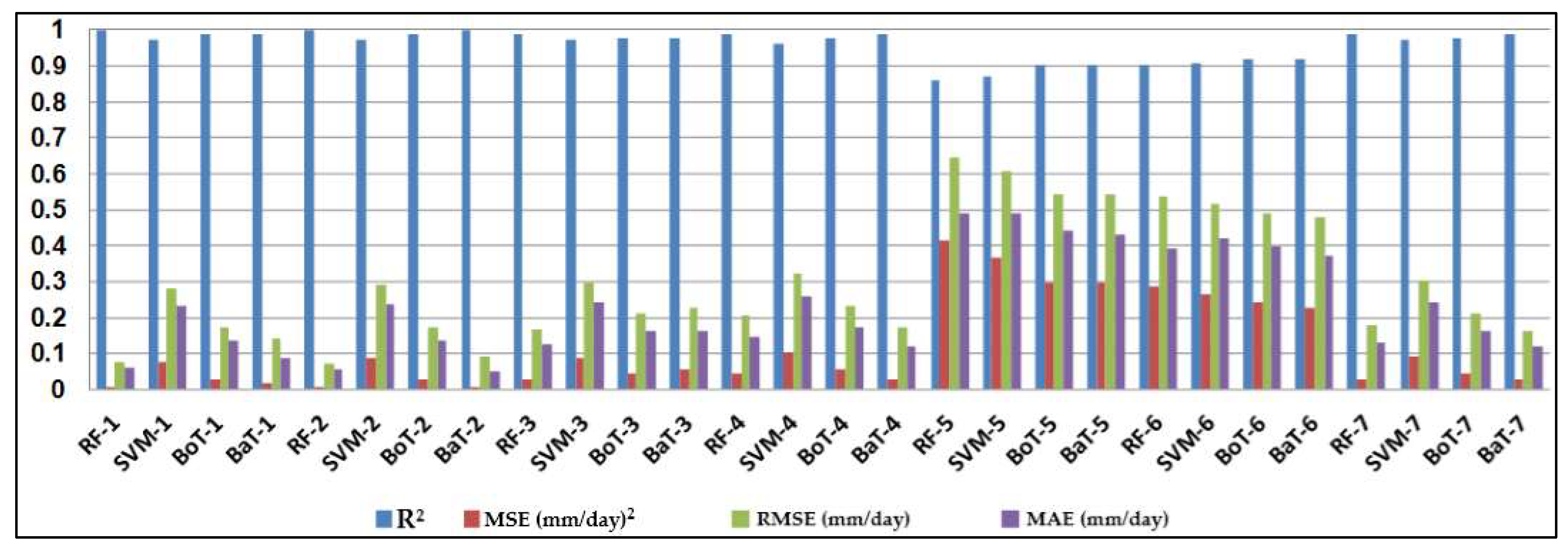
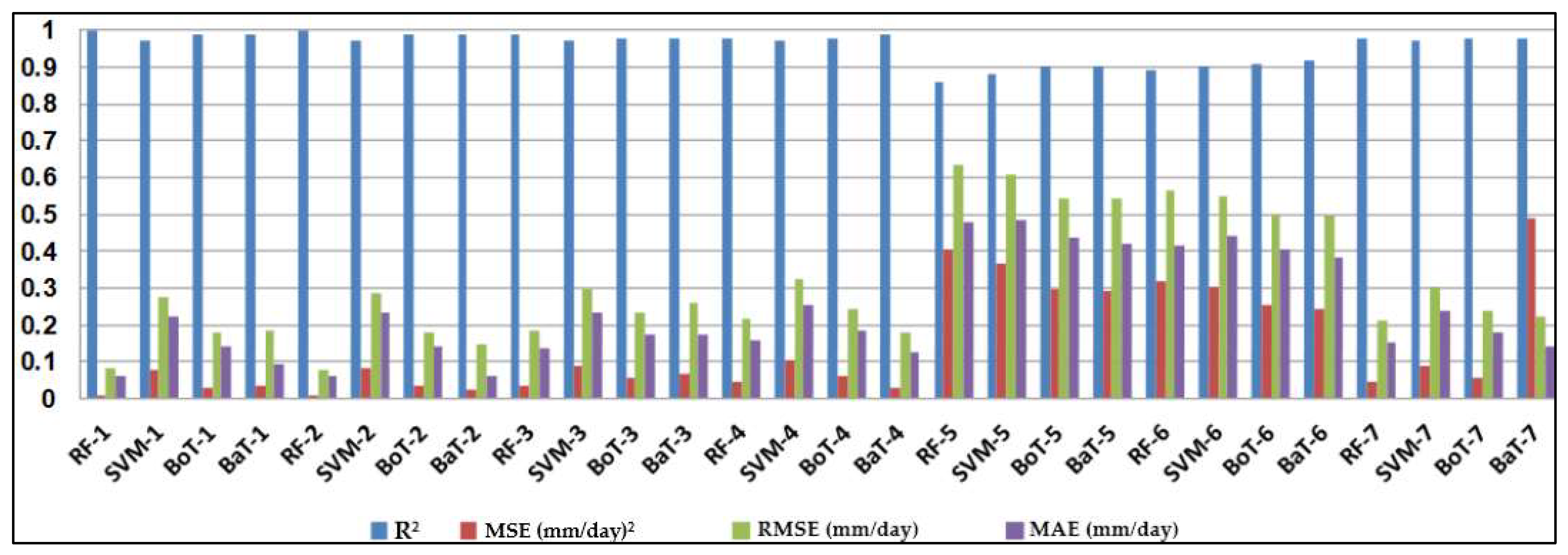
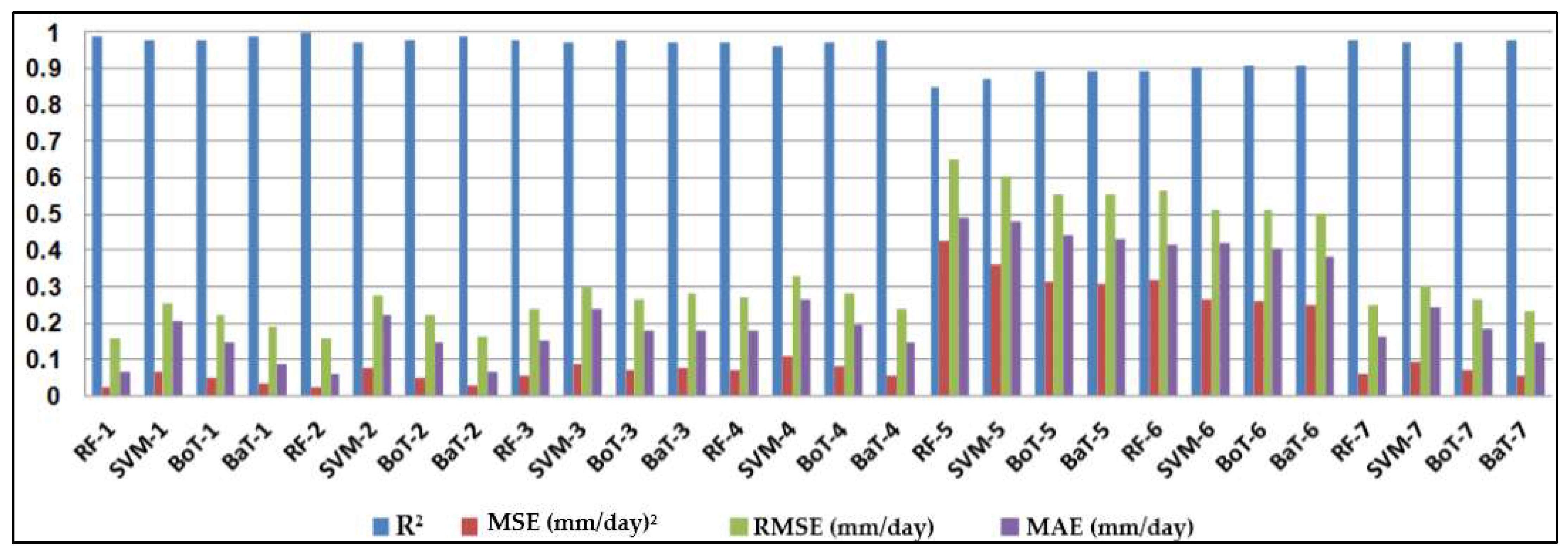
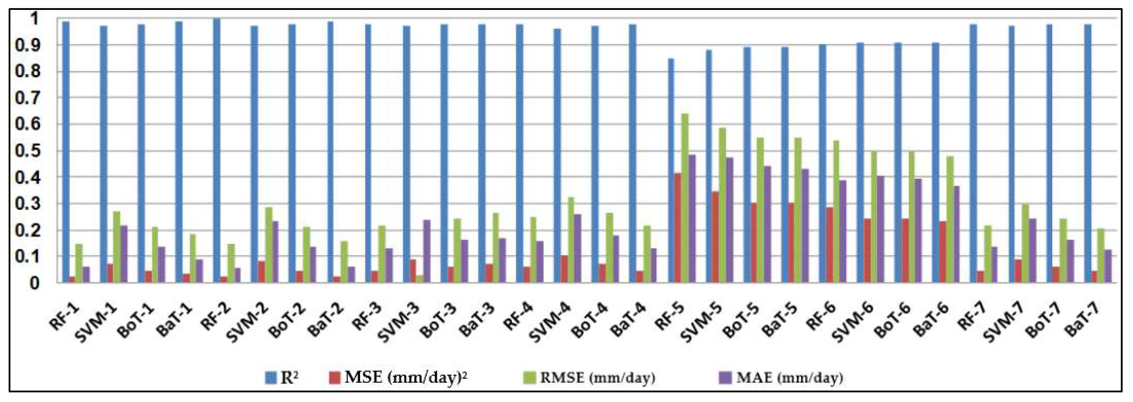
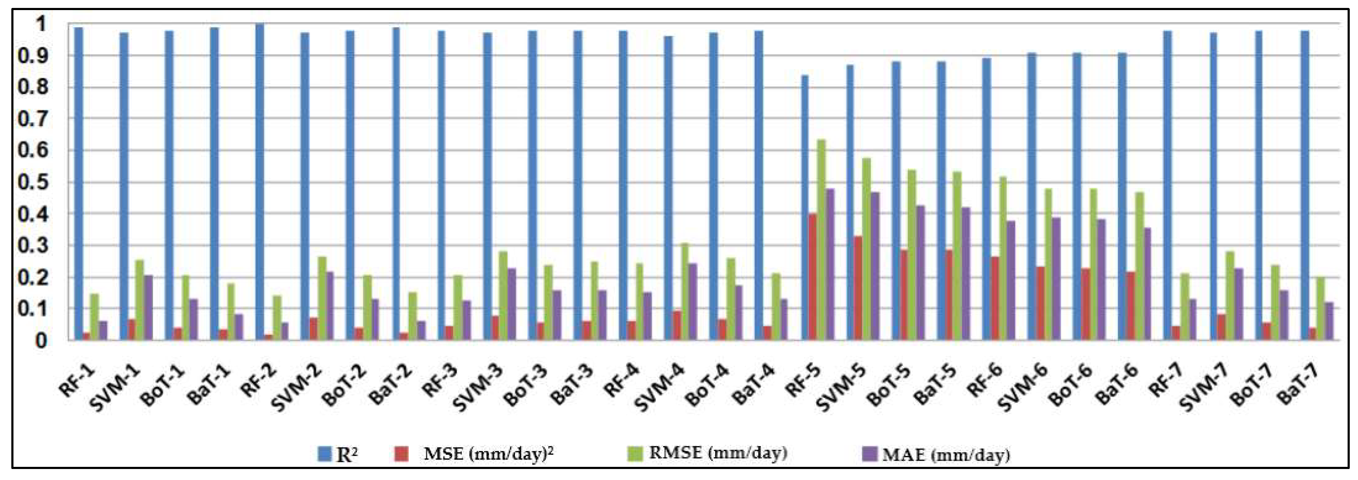
The most important step in using machine-learning models is evaluating their accuracy. Performance evaluation of the four soft computing models was conducted based on regression analysis using four statistical indices, namely mean absolute error (MAE), root mean square error (RMSE), mean square error (MSE), and coefficient of determination (R2).
3. Results
The utilized input scenarios for daily ET0 estimation are presented in Table 2. From the table, the first Scenario (M1) used full variables as inputs, while the seventh Scenario (M7) had only two variables, Tmean and SR. The performance metrics of the employed methods in estimating daily ET0 of the five stations are presented in the following sections.
Table 2.
Scenarios of input combinations used for daily ET0 estimation at study stations.
3.1. Qarah-Tapah Station
From Figure 2 and Table 3, the performance metrics of the employed methods in estimating the daily ET0 of the Qarah-Tapah station shows that the RF method had R2, MSE, RMSE, and MAE ranges from 0.86 (RF-5) to 1 (RF-1), from 0.05 (RF-2) to 0.414 (RF-5), from 0.074 (RF-2) to 0.643 (RF-5), and from 0.055 (RF-2) to 0.487 (RF-5), respectively. It is evident from the metrics’ ranges that the RF method was generally more successful in estimating the daily ET0 of the Qarah-Tapah station. Another finding is that for the RF method, there was a small difference between the first and second scenarios, and the second one produced the best accuracy. The other methods behaved differently, for example, the first and second input combinations provided the same accuracy for the BoT method. The M1 scenario had slightly better accuracy than the M2 for the SVM method, while the first scenario performed worse compared to latter for the BaT. This difference can be explained by the different working principles of the four implemented methods. The best estimates belonged to the RF method, followed by the BaT methods, while the SVM generally produced the worst ET0 estimates.
Figure 2.
The effectiveness of the applied models in daily ET0 estimation at the Qarah-Tapah station.
Table 3.
The effectiveness of the applied models in daily ET0 estimation at the Qarah-Tapah station during the testing period.
3.2. Mandali Station
The test performances of the RF, SVM, BoT, and BaT methods in estimating ET0 of the Mandali Station are reported in Figure 3 and Table 4. Here, it was also clear that the RF-2 model had the lowest MSE (0.024), RMSE (0.156), and MAE (0.059) followed by those of the RF-1 and BaT-2 models, while SVM produced the worst estimates, similar to the previous station.
Figure 3.
The effectiveness of the applied models in daily ET0 estimation at the Mandali station.
Table 4.
The effectiveness of the applied models in daily ET0 estimation at the Mandali station during the testing period.
3.3. Kalar Station
Figure 4 and Table 5 present the test performances of the implemented four methods in estimating ET0 of the Kalar Station. Similarly to Qarah-Tapah and Mandali stations, the RF-2 model provides the best performance with the lowest MSE (0.022), RMSE (0.148), and MAE (0.056) and the highest R2 (0.998), followed by those of RF-1 and BaT-2 models. In this station, the BaT and BoT ranked second and third, while the SVM was the least accurate model.
Figure 4.
The effectiveness of the applied models in daily ET0 estimation at the Kalar station.
Table 5.
The effectiveness of the applied models in daily ET0 estimation at the Kalar station during the testing period.
3.4. Iraq–Iran Station
Figure 5 and Table 6 give the performance metrics of the four methods in the test period of the Iraq–Iran Border station. In this station, RF-2 also ranked first by providing the lowest MSE (0.020), RMSE (0.143), and MAE (0.055) and the highest R2 (0.998), followed by those of the RF-1 and BaT-2 models. Here as well BoT and BaT performed superior to the SVM method. Again, the fifth scenario provided the worst results, while the first and second input scenarios had the best ET0 estimates.
Figure 5.
The effectiveness of the applied models in daily ET0 estimation at the Iraq–Iran Border station.
Table 6.
The effectiveness of the applied models in daily ET0 estimation at the Iraq–Iran Border station during the testing period.
3.5. Adhim Station
The performance measures of the RF, SVM, BoT, and BaT methods in estimation at the Adhim Station are presented in Figure 6 and Table 7. The RF-2 model had the lowest MSE (0.006), RMSE (0.078), and MAE (0.058), followed by those of the RF-1 and BaT-2 models. SVM generally produced the worst estimates, while BaT and BoT methods followed the RF in accuracy for estimating the daily ET0. Models including the first and/or scond scenarios perform the best, while models with the fifth combination had the worst results. In this station, BoT-1 had better accuracy than BoT-2 did; however, this difference was marginal.
Figure 6.
The effectiveness of the applied models in daily ET0 estimation at the Adhim station.
Table 7.
The effectiveness of the applied models in daily ET0 estimation at the Adhim station during the testing period.
Overall, the RF method, especially with the Tmax, Tmin, Tmean, and SR inputs, provided the best accuracy in estimating the daily ET0 of all stations. Its accuracy was followed by that of the BaT and BoT methods, while SVM had the worst accuracy. In most cases, the second input scenario provided the best accuracy in estimating the daily ET0. It is also worth noting that the seventh input scenario, having only Tmean and SR inputs, performed superior to the fourth, fifth, and sixth input scenarios. These results are contrary to those of [56], where a support vector machine (SVM) model was developed for ET0 estimation using limited climatic data (i.e., maximum and minimum temperature, wind speed, and solar radiation). The results in that study acknowledged that the SVM was useful for ET0 estimation with acceptable accuracy.
On the other hand, [66] used two machine-learning methods, random vector functional link (RVFL) and relevance vector machine (RVM), in modeling ET0 using limited climatic data, Tmax, Tmin, and extraterrestrial radiation with various input combinations and three data split scenarios. The study indicated that using only the temperature input (Tmin, Tmax) provided the worst ET0 estimations. Other studies also acknowledged similar results [67,68]. Another study found that temperature-based models involving temperature and Ra inputs offer promising results [61].
Figure 7 and Figure 8 illustrate the time variation and scatter plots of the best model (RF-2) estimates. It is clear from Figure 7 that the ET0 estimates by RF-2 were closely following the observed values. The models’ ranks from the best to worst are presented in Table 8. From Table 8, we can say that the first or second input scenarios, inlcuding Tmax, Tmin, Tmean, SR, WS, and RH; and Tmax, Tmin, Tmean and SR variables, respectively, generally provided the best estimates, while the fifth scenario, involving RH, WS, and Tmax, gave the worst ET0 estimates. The main reason of this might be the fact that the SR input is very effective for ET0, and not having it in this combination (fifth) and involving the WS parameter may worsen the estimation accuracy. Adding some input variables may negatively affect the variance and cause worse model accuracy in machine learning modeling. Here, adding WS might deteriorate the model’s performance, as this can be observed from the first and second input cases. From Table 8 it can also clearly be seen that for the Kalar Station, the first and second scenarios produced the best estimates, whereas the fifth scenario had the worst results. As clearly seen from Figure 8, the fit line of RF-2 overlapped the ideal line (1:1 line), and it had a high correlation for all stations. All these results highly recommend the RF method in estimating daily ET0.

Figure 7.
The temporal distribution of observed vs. estimated monthly ET0 values yielded by the best RF-2 model corresponding to M2 at (a) Qarah-Tapah, (b) Mandali, (c) Kalar, (d) Iraq–Iran Border, and (e) Adhim stations during the testing period.

Figure 8.
Scatter plots of the best RF-2 model corresponding to M2 for monthly ET0 estimation at (a) Qarah-Tapah, (b) Mandali, (c) Kalar, (d) Iraq–Iran Border, and (e) Adhim stations during the testing period.
Table 8.
Ranks of ML models based on the five stations.
4. Discussion
Evapotranspiration plays a significant role in the hydrological cycle and finds applications in water resource management, including irrigation, as well as in the assessment and surveillance of drought conditions [69,70,71,72,73,74,75,
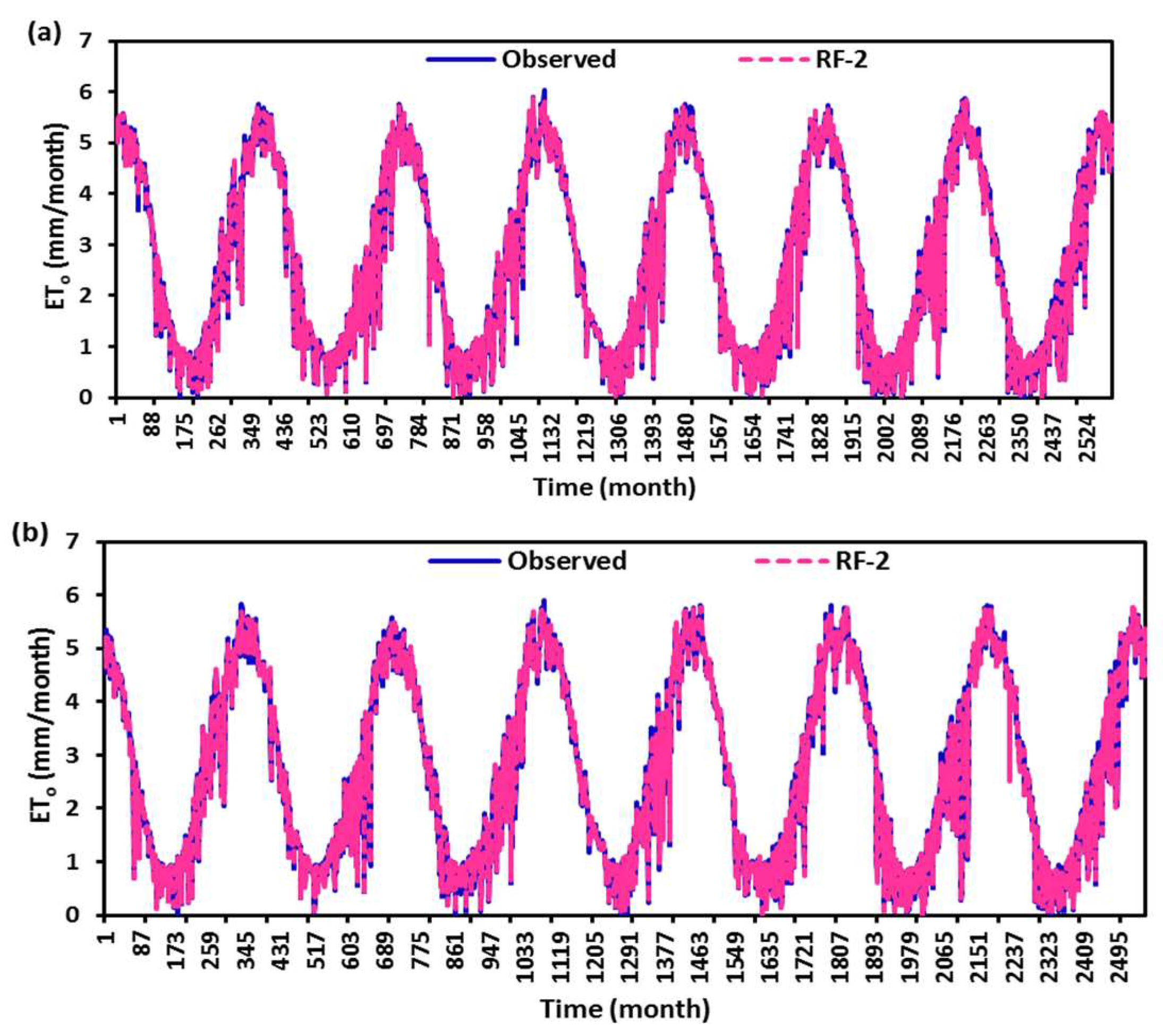
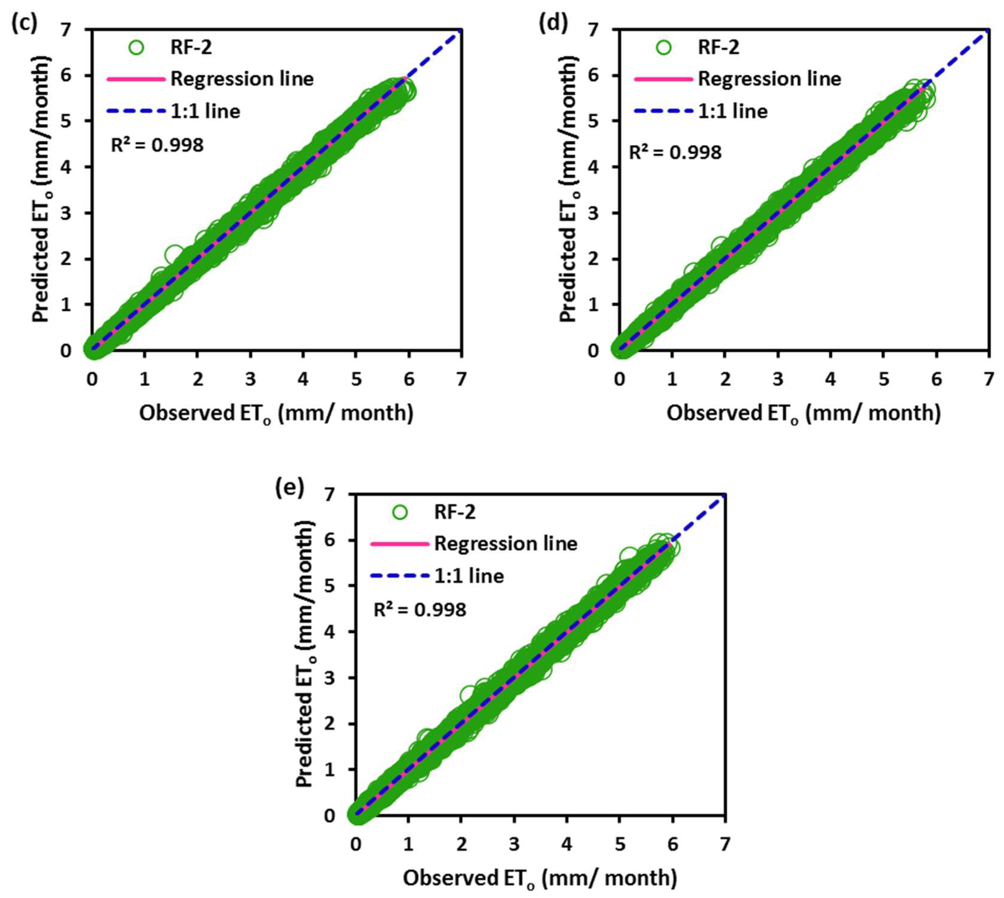
76]. Four different regression-based machine learning methods were compared for modeling daily reference evapotranspiration (ET0) for a semi-arid region (the Hemren catchment basin in Iraq). The comparison statistics indicated that the random forest method with Tmax, Tmin, Tmean, and SR inputs performed superior to the other methods in estimating the daily ET0 at all stations, while the SVM had the worst accuracy. Random forest (RF) is a popular machine-learning algorithm known for its strong predictive performance, minimal overfitting, and ease of interpretability. RF constructs multiple decision trees and combines them using a voting mechanism, resulting in robust generalization capabilities. One key feature of RF is its use of embedded methods for feature selection, which combines the strengths of filter and wrapper methods. Embedded methods are known for their high accuracy, excellent generalization, and interpretability. RF builds multiple decision trees, each using a random subset of data observations and features. This ensures that the trees are uncorrelated and less prone to overfitting. Each tree consists of a series of questions based on features, with each question dividing the data into two groups based on their similarity, ultimately determining the importance of each feature. In summary, RF is a powerful machine learning algorithm valued for its predictive abilities, robustness, and interpretability, making it a popular choice in various applications.
In [55], ET0 estimation was carried out using radial based artificial neural networks (RBNNs) and generalized regression artificial neural networks (GRNNs). The inputs for this estimation included daily mean relative humidity, sunshine duration, maximum and minimum air temperatures, mean air temperature, and wind speed. The study yielded the best R2 values of 0.868 and 0.889 for the RBNN and GRNN, respectively. Granata and Nunno [77] adopted two deep learning methods, NARX and LSTM, to model ET0. They experimented with various input combinations, including solar radiation, mean air temperature, sensible heat flux, relative humidity, and lagged ET0 values. The results showed R2 values of 0.687 and 0.837 as the best performance achieved by the LSTM and NARX models, respectively. The table data in Table 3, Table 4, Table 5, Table 6 and Table 7 clearly demonstrate that the proposed methods achieved remarkable success in modeling ET0.
5. Conclusions
In this study, the applicability of four different regression-based machine learning methods in estimating ET0 was investigated. Climatic data from five stations located in a semi-arid region of Iraq was used as inputs to the models. According to comparison statistics (R2, MSE, RMSE, and MAE) and graphical inspection, the random forest model offered the best ET0 estimates in all stations, while the SVM provided the worst accuracy. Employing various combinations of climatic inputs revealed that the models with Tmax, Tmin, Tmean, and SR inputs produced the best estimations. The best random forest model with Tmax, Tmin, Tmean, and SR improved the estimation accuracy of the SVM, BoT, and BaT models by 94%, 83%, and 38% for Qarah-Tapah, by 68%, 50%, and 8% for Mandali, by 73%, 49%, and 8% for Kalar, by 72%, 51%, and 9% for Iran–Iraq Border, and by 93%, 81%, and 73% for Adhim with respect to RMSE in the test period, respectively. The outcomes of the study recommend random forest for estimating ET0 in a semi-arid region. The study used data from one region, and more data can be used to assess the regression-based machine learning methods in future studies. The regression-based methods considered in this study may be compared with more complex machine learning methods.
Author Contributions
Conceptualization: S.S.S., A.M.S.A.-J., O.K., and A.E.; data creation: O.K. and S.S.S.; formal analysis: O.K. and S.S.S.; investigation: O.K. and A.M.S.A.-J.; methodology: S.S.S. and A.M.S.A.-J.; software: A.E. and O.K.; validation: S.S.S. and O.K.; writing—original draft: O.K., A.M.S.A.-J. and S.S.S.; writing—review and editing, S.S.S., A.M.S.A.-J., O.K., A.E and M.Z.-K. All authors have read and agreed to the published version of the manuscript.
Funding
This research received no external funding.
Data Availability Statement
It will be available on request.
Conflicts of Interest
The authors declare no conflict of interest.
References
- French, A.; Hunsaker, D.; Bounoua, L.; Karnieli, A.; Luckett, W.; Strand, R. Remote Sensing of Evapotranspiration over the Central Arizona Irrigation and Drainage District, USA. Agronomy 2018, 8, 278. [Google Scholar] [CrossRef]
- Calera, A.; Campos, I.; Osann, A.; D’Urso, G.; Menenti, M. Remote Sensing for Crop Water Management: From ET Modelling to Services for the End Users. Sensors 2017, 17, 1104. [Google Scholar] [CrossRef] [PubMed]
- Anderson, M.C.; Zolin, C.A.; Sentelhas, P.C.; Hain, C.R.; Semmens, K.; Tugrul Yilmaz, M.; Gao, F.; Otkin, J.A.; Tetrault, R. The Evaporative Stress Index as an indicator of agricultural drought in Brazil: An assessment based on crop yield impacts. Remote Sens. Environ. 2016, 174, 82–99. [Google Scholar] [CrossRef]
- Senay, G.B.; Velpuri, N.M.; Bohms, S.; Budde, M.; Young, C.; Rowland, J.; Verdin, J.P. Drought Monitoring and Assessment. In Hydro-Meteorological Hazards, Risks and Disasters; Shroder, J.F., Paron, P., Di Baldassarre, G., Eds.; Elsevier: Amsterdam, The Netherlands, 2015; pp. 233–262. [Google Scholar]
- Yusuf, B.; Al-Janabi, A.M.S.; Ghazali, A.H.; Al-Ani, I. Variations of infiltration capacity with flow hydraulic parameters in permeable stormwater channels. ISH J. Hydraul. Eng. 2022, 28, 234–242. [Google Scholar] [CrossRef]
- Khan, A.; Stöckle, C.O.; Nelson, R.L.; Peters, T.; Adam, J.C.; Lamb, B.; Chi, J.; Waldo, S. Estimating Biomass and Yield Using METRIC Evapotranspiration and Simple Growth Algorithms. Agron. J. 2019, 111, 536–544. [Google Scholar] [CrossRef]
- Doorenbos, J.; Kassam, A.H.; Bentvelsen, C.; Uittenbogaard, G. Yield Response to Water. In Irrigation and Agricultural Development; Johl, S.S., Ed.; Pergamon Press: Oxford, UK, 1980; pp. 257–280. [Google Scholar]
- Trenberth, K.E.; Smith, L.; Qian, T.; Dai, A.; Fasullo, J. Estimates of the Global Water Budget and Its Annual Cycle Using Observational and Model Data. J. Hydrometeorol. 2007, 8, 758–769. [Google Scholar] [CrossRef]
- Wang, K.; Dickinson, R.E. A review of global terrestrial evapotranspiration: Observation, modeling, climatology, and climatic variability. Rev. Geophys. 2012, 50. [Google Scholar] [CrossRef]
- Granata, F. Evapotranspiration evaluation models based on machine learning algorithms—A comparative study. Agric. Water Manag. 2019, 217, 303–315. [Google Scholar] [CrossRef]
- Jung, M.; Reichstein, M.; Ciais, P.; Seneviratne, S.I.; Sheffield, J.; Goulden, M.L.; Bonan, G.; Cescatti, A.; Chen, J.; de Jeu, R.; et al. Recent decline in the global land evapotranspiration trend due to limited moisture supply. Nature 2010, 467, 951–954. [Google Scholar] [CrossRef]
- Mueller, B.; Hirschi, M.; Jimenez, C.; Ciais, P.; Dirmeyer, P.A.; Dolman, A.J.; Fisher, J.B.; Jung, M.; Ludwig, F.; Maignan, F.; et al. Benchmark products for land evapotranspiration: LandFlux-EVAL multi-data set synthesis. Hydrol. Earth Syst. Sci. 2013, 17, 3707–3720. [Google Scholar] [CrossRef]
- Zeng, Z.; Piao, S.; Lin, X.; Yin, G.; Peng, S.; Ciais, P.; Myneni, R.B. Global evapotranspiration over the past three decades: Estimation based on the water balance equation combined with empirical models. Environ. Res. Lett. 2012, 7, 14026. [Google Scholar] [CrossRef]
- Zeng, Z.; Wang, T.; Zhou, F.; Ciais, P.; Mao, J.; Shi, X.; Piao, S. A worldwide analysis of spatiotemporal changes in water balance-based evapotranspiration from 1982 to 2009. J. Geophys. Res. Atmos. 2014, 119, 1186–1202. [Google Scholar] [CrossRef]
- Al-Janabi, A.M.S.; Halim Ghazali, A.; Yusuf, B. Modified models for better prediction of infiltration rates in trapezoidal permeable stormwater channels. Hydrol. Sci. J. 2019, 64, 1918–1931. [Google Scholar] [CrossRef]
- Fisher, J.B.; Melton, F.; Middleton, E.; Hain, C.; Anderson, M.; Allen, R.; McCabe, M.F.; Hook, S.; Baldocchi, D.; Townsend, P.A.; et al. The future of evapotranspiration: Global requirements for ecosystem functioning, carbon and climate feedbacks, agricultural management, and water resources. Water Resour. Res. 2017, 53, 2618–2626. [Google Scholar] [CrossRef]
- Petropoulos, G.P.; Ireland, G.; Lamine, S.; Griffiths, H.M.; Ghilain, N.; Anagnostopoulos, V.; North, M.R.; Srivastava, P.K.; Georgopoulou, H. Operational evapotranspiration estimates from SEVIRI in support of sustainable water management. Int. J. Appl. Earth Obs. Geoinf. 2016, 49, 175–187. [Google Scholar] [CrossRef]
- Jung, M.; Reichstein, M.; Margolis, H.A.; Cescatti, A.; Richardson, A.D.; Arain, M.A.; Arneth, A.; Bernhofer, C.; Bonal, D.; Chen, J.; et al. Global patterns of land-atmosphere fluxes of carbon dioxide, latent heat, and sensible heat derived from eddy covariance, satellite, and meteorological observations. J. Geophys. Res. 2011, 116. [Google Scholar] [CrossRef]
- Xu, T.; Guo, Z.; Liu, S.; He, X.; Meng, Y.; Xu, Z.; Xia, Y.; Xiao, J.; Zhang, Y.; Ma, Y.; et al. Evaluating Different Machine Learning Methods for Upscaling Evapotranspiration from Flux Towers to the Regional Scale. J. Geophys. Res. Atmos. 2018, 123, 8674–8690. [Google Scholar] [CrossRef]
- Cui, G.; Zhu, J. Infiltration model in sloping layered soils and guidelines for model parameter estimation. Hydrol. Sci. J. 2017, 62, 2222–2237. [Google Scholar] [CrossRef]
- Zhao, B.; Mao, K.; Cai, Y.; Shi, J.; Li, Z.; Qin, Z.; Meng, X.; Shen, X.; Guo, Z. A combined Terra and Aqua MODIS land surface temperature and meteorological station data product for China from 2003 to 2017. Earth Syst. Sci. Data 2020, 12, 2555–2577. [Google Scholar] [CrossRef]
- Ma, Y.; Liu, S.; Song, L.; Xu, Z.; Liu, Y.; Xu, T.; Zhu, Z. Estimation of daily evapotranspiration and irrigation water efficiency at a Landsat-like scale for an arid irrigation area using multi-source remote sensing data. Remote Sens. Environ. 2018, 216, 715–734. [Google Scholar] [CrossRef]
- Miralles, D.G.; Holmes, T.R.H.; De Jeu, R.A.M.; Gash, J.H.; Meesters, A.G.C.A.; Dolman, A.J. Global land-surface evaporation estimated from satellite-based observations. Hydrol. Earth Syst. Sci. 2011, 15, 453–469. [Google Scholar] [CrossRef]
- Yao, Y.; Liang, S.; Li, X.; Chen, J.; Wang, K.; Jia, K.; Cheng, J.; Jiang, B.; Fisher, J.B.; Mu, Q.; et al. A satellite-based hybrid algorithm to determine the Priestley–Taylor parameter for global terrestrial latent heat flux estimation across multiple biomes. Remote Sens. Environ. 2015, 165, 216–233. [Google Scholar] [CrossRef]
- Zhang, K.; Kimball, J.S.; Running, S.W. A review of remote sensing based actual evapotranspiration estimation. WIREs Water 2016, 3, 834–853. [Google Scholar] [CrossRef]
- Bateni, S.M.; Entekhabi, D.; Jeng, D.-S. Variational assimilation of land surface temperature and the estimation of surface energy balance components. J. Hydrol. 2013, 481, 143–156. [Google Scholar] [CrossRef]
- He, X.; Xu, T.; Xia, Y.; Bateni, S.M.; Guo, Z.; Liu, S.; Mao, K.; Zhang, Y.; Feng, H.; Zhao, J. A Bayesian Three-Cornered Hat (BTCH) Method: Improving the Terrestrial Evapotranspiration Estimation. Remote Sens. 2020, 12, 878. [Google Scholar] [CrossRef]
- Lu, Y.; Steele-Dunne, S.C.; Farhadi, L.; van de Giesen, N. Mapping Surface Heat Fluxes by Assimilating SMAP Soil Moisture and GOES Land Surface Temperature Data. Water Resour. Res. 2017, 53, 10858–10877. [Google Scholar] [CrossRef]
- Xu, T.; Bateni, S.M.; Liang, S.; Entekhabi, D.; Mao, K. Estimation of surface turbulent heat fluxes via variational assimilation of sequences of land surface temperatures from Geostationary Operational Environmental Satellites. J. Geophys. Res. Atmos. 2014, 119, 10780–10798. [Google Scholar] [CrossRef]
- Xia, Y.; Hao, Z.; Shi, C.; Li, Y.; Meng, J.; Xu, T.; Wu, X.; Zhang, B. Regional and Global Land Data Assimilation Systems: Innovations, Challenges, and Prospects. J. Meteorol. Res. 2019, 33, 159–189. [Google Scholar] [CrossRef]
- Zhang, B.; Xia, Y.; Long, B.; Hobbins, M.; Zhao, X.; Hain, C.; Li, Y.; Anderson, M.C. Evaluation and comparison of multiple evapotranspiration data models over the contiguous United States: Implications for the next phase of NLDAS (NLDAS-Testbed) development. Agric. For. Meteorol. 2020, 280, 107810. [Google Scholar] [CrossRef]
- Long, D.; Longuevergne, L.; Scanlon, B.R. Uncertainty in evapotranspiration from land surface modeling, remote sensing, and GRACE satellites. Water Resour. Res. 2014, 50, 1131–1151. [Google Scholar] [CrossRef]
- Kalma, J.D.; McVicar, T.R.; McCabe, M.F. Estimating Land Surface Evaporation: A Review of Methods Using Remotely Sensed Surface Temperature Data. Surv. Geophys. 2008, 29, 421–469. [Google Scholar] [CrossRef]
- Velpuri, N.M.; Senay, G.B.; Singh, R.K.; Bohms, S.; Verdin, J.P. A comprehensive evaluation of two MODIS evapotranspiration products over the conterminous United States: Using point and gridded FLUXNET and water balance ET. Remote Sens. Environ. 2013, 139, 35–49. [Google Scholar] [CrossRef]
- Anapalli, S.S.; Ahuja, L.R.; Gowda, P.H.; Ma, L.; Marek, G.; Evett, S.R.; Howell, T.A. Simulation of crop evapotranspiration and crop coefficients with data in weighing lysimeters. Agric. Water Manag. 2016, 177, 274–283. [Google Scholar] [CrossRef]
- Liu, X.; Xu, C.; Zhong, X.; Li, Y.; Yuan, X.; Cao, J. Comparison of 16 models for reference crop evapotranspiration against weighing lysimeter measurement. Agric. Water Manag. 2017, 184, 145–155. [Google Scholar] [CrossRef]
- Stanhill, G. Evapotranspiration. In Encyclopedia of Soils in the Environment; Hillel, D., Rosenzweig, C., Powlson, D., Scow, K., Singer, M., Sparks, D., Eds.; Academic Press: Cambridge, MA, USA, 2005; pp. 502–506. [Google Scholar]
- Chen, Z.; Shi, R.; Zhang, S. An artificial neural network approach to estimate evapotranspiration from remote sensing and AmeriFlux data. Front. Earth Sci. 2012, 7, 103–111. [Google Scholar] [CrossRef]
- Sihag, P.; Kumar, M.; Sammen, S.S. Predicting the infiltration characteristics for semi-arid regions using regression trees. Water Supply 2021, 21, 2583–2595. [Google Scholar] [CrossRef]
- Malik, A.; Tikhamarine, Y.; Sammen, S.S.; Abba, S.I.; Shahid, S. Prediction of meteorological drought by using hybrid support vector regression optimized with HHO versus PSO algorithms. Environ. Sci. Pollut. Res. 2021, 28, 39139–39158. [Google Scholar] [CrossRef]
- Sammen, S.S.; Ehteram, M.; Abba, S.I.; Abdulkadir, R.A.; Ahmed, A.N.; El-Shafie, A. A new soft computing model for daily streamflow forecasting. Stoch. Environ. Res. Risk Assess. 2021, 35, 2479–2491. [Google Scholar] [CrossRef]
- Abba, S.I.; Abdulkadir, R.A.; Sammen, S.S.; Pham, Q.B.; Lawan, A.A.; Esmaili, P.; Malik, A.; Al-Ansari, N. Integrating feature extraction approaches with hybrid emotional neural networks for water quality index modeling. Appl. Soft Comput. 2021, 114, 108036. [Google Scholar] [CrossRef]
- Ebtehaj, I.; Sammen, S.S.; Sidek, L.M.; Malik, A.; Sihag, P.; Al-Janabi, A.M.S.; Chau, K.-W.; Bonakdari, H. Prediction of daily water level using new hybridized GS-GMDH and ANFIS-FCM models. Eng. Appl. Comput. Fluid Mech. 2021, 15, 1343–1361. [Google Scholar] [CrossRef]
- Hashim, B.M.; Al Maliki, A.; Alraheem, E.A.; Al-Janabi, A.M.S.; Halder, B.; Yaseen, Z.M. Temperature and precipitation trend analysis of the Iraq Region under SRES scenarios during the twenty-first century. Theor. Appl. Climatol. 2022, 148, 881–898. [Google Scholar] [CrossRef]
- Mdegela, L.; Municio, E.; De Bock, Y.; Luhanga, E.; Leo, J.; Mannens, E. Extreme Rainfall Event Classification Using Machine Learning for Kikuletwa River Floods. Water 2023, 15, 1021. [Google Scholar] [CrossRef]
- Sihag, P.; Dursun, O.F.; Sammen, S.S.; Malik, A.; Chauhan, A. Prediction of aeration efficiency of Parshall and Modified Venturi flumes: Application of soft computing versus regression models. Water Supply 2021, 21, 4068–4085. [Google Scholar] [CrossRef]
- Alomari, N.K.; Sihag, P.; Sami Al-Janabi, A.M.; Yusuf, B. Modeling of scour depth and length of a diversion channel flow system with soft computing techniques. Water Supply 2023, 23, 1267–1283. [Google Scholar] [CrossRef]
- Sammen, S.S.; Ghorbani, M.A.; Malik, A.; Tikhamarine, Y.; AmirRahmani, M.; Al-Ansari, N.; Chau, K.-W. Enhanced Artificial Neural Network with Harris Hawks Optimization for Predicting Scour Depth Downstream of Ski-Jump Spillway. Appl. Sci. 2020, 10, 5160. [Google Scholar] [CrossRef]
- Granata, F.; Di Nunno, F.; Modoni, G. Hybrid Machine Learning Models for Soil Saturated Conductivity Prediction. Water 2022, 14, 1729. [Google Scholar] [CrossRef]
- Ehteram, M.; Sammen, S.S.; Panahi, F.; Sidek, L.M. A hybrid novel SVM model for predicting CO2 emissions using Multiobjective Seagull Optimization. Environ. Sci. Pollut. Res. 2021, 28, 66171–66192. [Google Scholar] [CrossRef]
- Abba, S.I.; Abdulkadir, R.A.; Sammen, S.S.; Usman, A.G.; Meshram, S.G.; Malik, A.; Shahid, S. Comparative implementation between neuro-emotional genetic algorithm and novel ensemble computing techniques for modelling dissolved oxygen concentration. Hydrol. Sci. J. 2021, 66, 1584–1596. [Google Scholar] [CrossRef]
- Alali, Y.; Harrou, F.; Sun, Y. Unlocking the Potential of Wastewater Treatment: Machine Learning Based Energy Consumption Prediction. Water 2023, 15, 2349. [Google Scholar] [CrossRef]
- Ni, J.; Liu, R.; Li, Y.; Tang, G.; Shi, P. An Improved Transfer Learning Model for Cyanobacterial Bloom Concentration Prediction. Water 2022, 14, 1300. [Google Scholar] [CrossRef]
- Yang, F.; White, M.A.; Michaelis, A.R.; Ichii, K.; Hashimoto, H.; Votava, P.; Zhu, A.-X.; Nemani, R.R. Prediction of Continental-Scale Evapotranspiration by Combining MODIS and AmeriFlux Data Through Support Vector Machine. IEEE Trans. Geosci. Remote Sens. 2006, 44, 3452–3461. [Google Scholar] [CrossRef]
- Ladlani, I.; Houichi, L.; Djemili, L.; Heddam, S.; Belouz, K. Modeling daily reference evapotranspiration (ET0) in the north of Algeria using generalized regression neural networks (GRNN) and radial basis function neural networks (RBFNN): A comparative study. Meteorol. Atmos. Phys. 2012, 118, 163–178. [Google Scholar] [CrossRef]
- Wen, X.; Si, J.; He, Z.; Wu, J.; Shao, H.; Yu, H. Support-Vector-Machine-Based Models for Modeling Daily Reference Evapotranspiration with Limited Climatic Data in Extreme Arid Regions. Water Resour. Manag. 2015, 29, 3195–3209. [Google Scholar] [CrossRef]
- Antonopoulos, V.Z.; Antonopoulos, A.V. Daily reference evapotranspiration estimates by artificial neural networks technique and empirical equations using limited input climate variables. Comput. Electron. Agric. 2017, 132, 86–96. [Google Scholar] [CrossRef]
- Adnan, M.; Latif, M.A.; Nazir, M. Estimating Evapotranspiration using Machine Learning Techniques. Int. J. Adv. Comput. Sci. Appl. 2017, 8, 108–113. [Google Scholar] [CrossRef]
- Carter, C.; Liang, S. Evaluation of ten machine learning methods for estimating terrestrial evapotranspiration from remote sensing. Int. J. Appl. Earth Obs. Geoinf. 2019, 78, 86–92. [Google Scholar] [CrossRef]
- Özgür, A.; Yamaç, S.S. Modelling of daily reference evapotranspiration using deep neural network in different climates. arXiv 2020, arXiv:2006.01760. [Google Scholar]
- Wu, L.; Peng, Y.; Fan, J.; Wang, Y. Machine learning models for the estimation of monthly mean daily reference evapotranspiration based on cross-station and synthetic data. Hydrol. Res. 2019, 50, 1730–1750. [Google Scholar] [CrossRef]
- Wu, T.; Zhang, W.; Jiao, X.; Guo, W.; Hamoud, Y.A. Comparison of five Boosting-based models for estimating daily reference evapotranspiration with limited meteorological variables. PLoS ONE 2020, 15, e0235324. [Google Scholar] [CrossRef]
- Shiri, J.; Zounemat-Kermani, M.; Kisi, O.; Mohsenzadeh Karimi, S. Comprehensive assessment of 12 soft computing approaches for modelling reference evapotranspiration in humid locations. Meteorol. Appl. 2020, 27, e1841. [Google Scholar] [CrossRef]
- Zounemat-Kermani, M.; Batelaan, O.; Fadaee, M.; Hinkelmann, R. Ensemble machine learning paradigms in hydrology: A review. J. Hydrol. 2021, 598, 126266. [Google Scholar] [CrossRef]
- Friedman, J.H. Stochastic gradient boosting. Comput. Stat. Data Anal. 2002, 38, 367–378. [Google Scholar] [CrossRef]
- Mostafa, R.R.; Kisi, O.; Adnan, R.M.; Sadeghifar, T.; Kuriqi, A. Modeling Potential Evapotranspiration by Improved Machine Learning Methods Using Limited Climatic Data. Water 2023, 15, 486. [Google Scholar] [CrossRef]
- Dimitriadou, S.; Nikolakopoulos, K.G. Multiple Linear Regression Models with Limited Data for the Prediction of Reference Evapotranspiration of the Peloponnese, Greece. Hydrology 2022, 9, 124. [Google Scholar] [CrossRef]
- Dimitriadou, S.; Nikolakopoulos, K.G. Artificial Neural Networks for the Prediction of the Reference Evapotranspiration of the Peloponnese Peninsula, Greece. Water 2022, 14, 2027. [Google Scholar] [CrossRef]
- Vangelis, H.; Tigkas, D.; Tsakiris, G. The effect of PET method on Reconnaissance Drought Index (RDI) calculation. J. Arid. Environ. 2013, 88, 130–140. [Google Scholar] [CrossRef]
- Tegos, A.; Stefanidis, S.; Cody, J.; Koutsoyiannis, D. On the Sensitivity of Standardized-Precipitation-Evapotranspiration and Aridity Indexes Using Alternative Potential Evapotranspiration Models. Hydrology 2023, 10, 64. [Google Scholar] [CrossRef]
- Sang, L.; Zhu, G.; Xu, Y.; Sun, Z.; Zhang, Z.; Tong, H. Effects of Agricultural Large-And Medium-Sized Reservoirs on Hydrologic Processes in the Arid Shiyang River Basin, Northwest China. Water Resour. Res. 2023, 59, 2. [Google Scholar] [CrossRef]
- Li, J.; Wang, Z.; Wu, X.; Xu, C.; Guo, S.; Chen, X. Toward Monitoring Short-Term Droughts Using a Novel Daily Scale, Standardized Antecedent Precipitation Evapotranspiration Index. J. Hydrometeorol. 2020, 21, 891–908. [Google Scholar] [CrossRef]
- Yin, L.; Wang, L.; Keim, B.D.; Konsoer, K.; Yin, Z.; Liu, M.; Zheng, W. Spatial and wavelet analysis of precipitation and river discharge during operation of the Three Gorges Dam, China. Ecol. Indic. 2023, 154, 110837. [Google Scholar] [CrossRef]
- Liu, Z.; Xu, J.; Liu, M.; Yin, Z.; Liu, X.; Yin, L.; Zheng, W. Remote sensing and geostatistics in urban water-resource monitoring: A review. Mar. Freshw. Res. 2023. [Google Scholar] [CrossRef]
- Tian, H.; Huang, N.; Niu, Z.; Qin, Y.; Pei, J.; Wang, J. Mapping Winter Crops in China with Multi-Source Satellite Imagery and Phenology-Based Algorithm. Remote Sens. 2019, 11, 820. [Google Scholar] [CrossRef]
- Wu, B.; Quan, Q.; Yang, S.; Dong, Y. A social-ecological coupling model for evaluating the human-water relationship in basins within the Budyko framework. J. Hydrol. 2023, 619, 129361. [Google Scholar] [CrossRef]
- Granata, F.; Nunno, F.D. Forecasting evapotranspiration in different climates using ensembles of recurrent neural networks. Agric. Water Manag. 2021, 255, 107040. [Google Scholar] [CrossRef]
Disclaimer/Publisher’s Note: The statements, opinions and data contained in all publications are solely those of the individual author(s) and contributor(s) and not of MDPI and/or the editor(s). MDPI and/or the editor(s) disclaim responsibility for any injury to people or property resulting from any ideas, methods, instructions or products referred to in the content. |
© 2023 by the authors. Licensee MDPI, Basel, Switzerland. This article is an open access article distributed under the terms and conditions of the Creative Commons Attribution (CC BY) license (https://creativecommons.org/licenses/by/4.0/).