

Two-Parameter Probability Distributions: Methods, Techniques and Comparative Analysis


Abstract
:1. Introduction
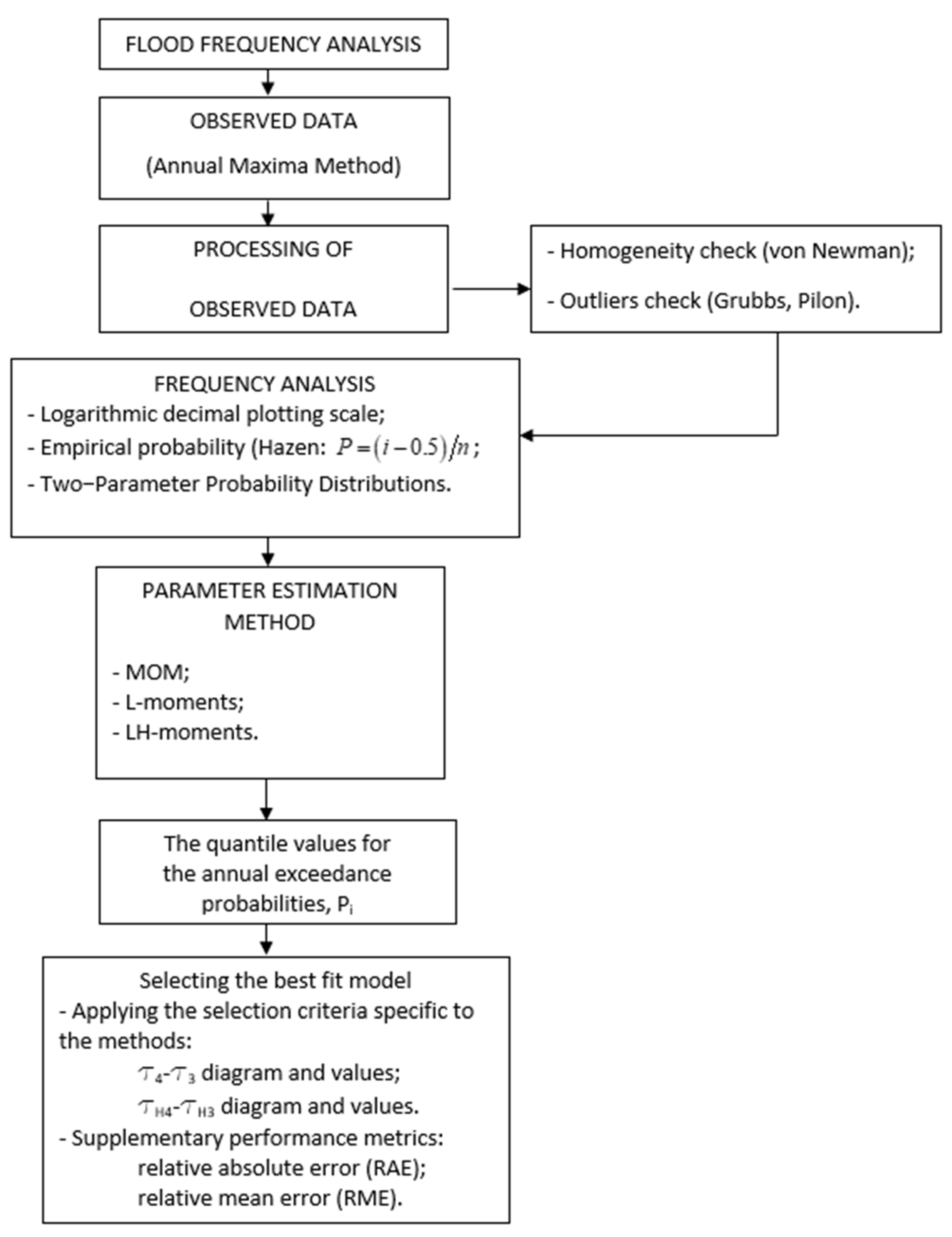
2. Methods
2.1. Density, Cumulative, and Inverse Functions
2.2. Relation between Parameters and Constraints for the Analyzed Methods
2.2.1. Pearson V Distribution (PV2)
2.2.2. Chi Distribution (CH2)
2.2.3. Inverse Chi Distribution (ICH2)
2.2.4. Gamma Distribution (Γ2)
2.2.5. Log-Normal Distribution (LN2)
2.2.6. Gumbel (G)
2.2.7. Logistic (L2)
2.2.8. Log-Logistic (LL2)
2.2.9. Exponential Shifted Distribution (E2)
2.2.10. Rayleigh Distribution (R2)
2.2.11. Weibull Distribution (W2)
2.2.12. Fréchet Distribution (F2)
2.2.13. Generalized Exponential Distribution (EG)
3. Study Area and Data
4. Results and Discussion
4.1. Verification of Independence, Stationarity, and Homogeneity
4.2. Quantile Estimation
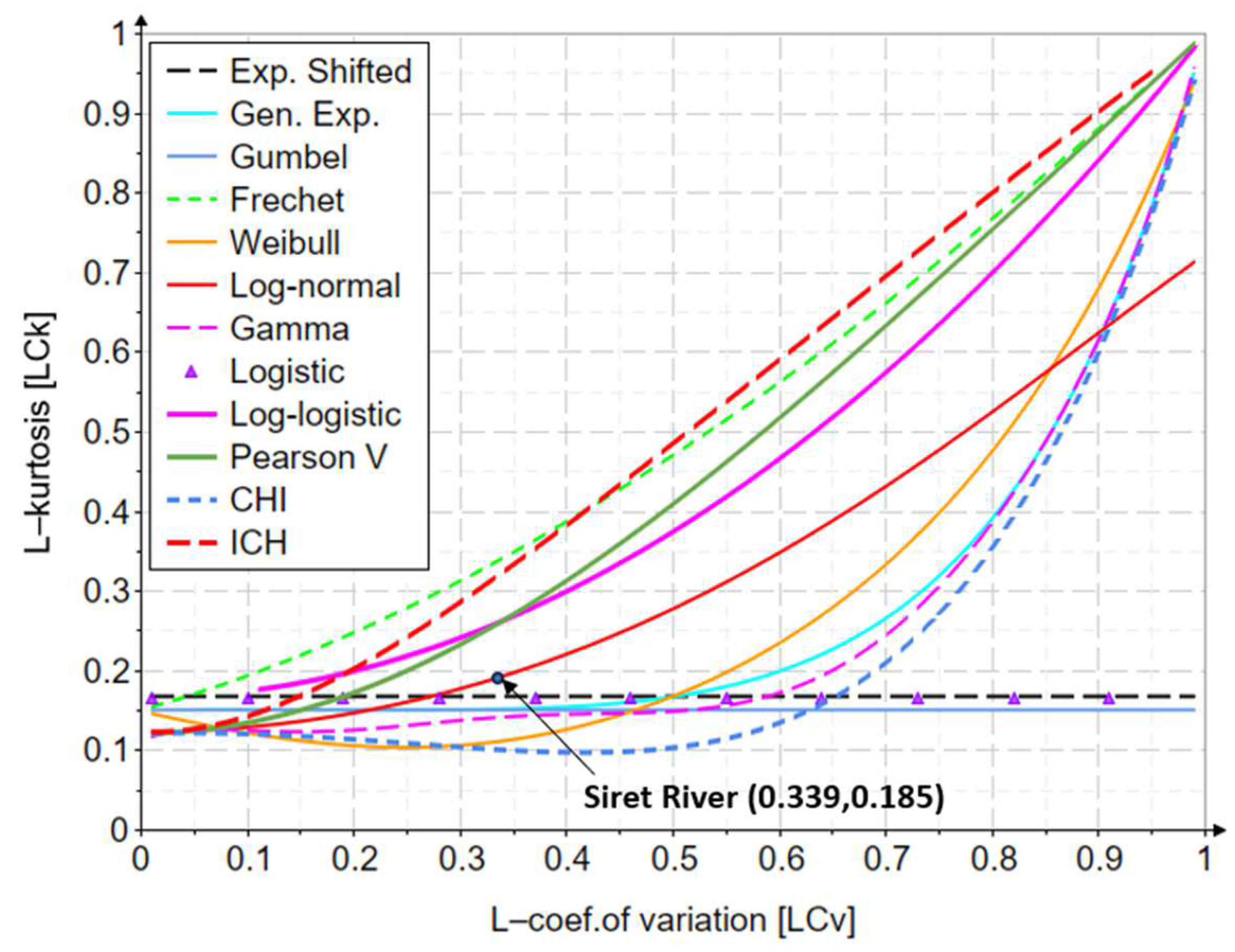
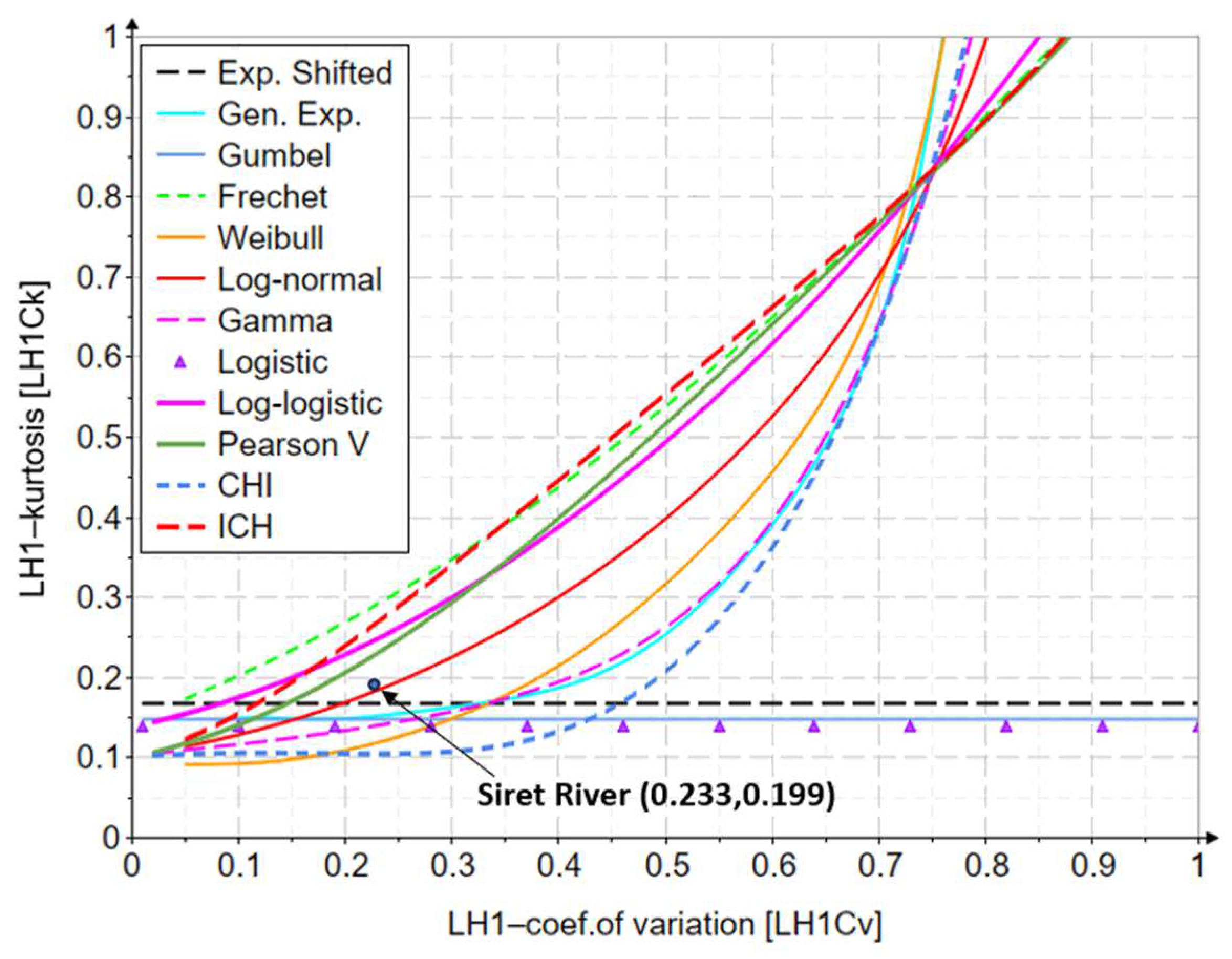
4.3. Performance Criterion
4.4. The Influence of the Variability of the Length of the Recorded Series
4.5. Confidence Interval
5. Conclusions
6. Future Directions
Author Contributions
Funding
Data Availability Statement
Conflicts of Interest
Nomenclature
| MOM | The method of ordinary moments |
| L-moments | The method of linear moments |
| LH-moments | The method of higher order linear moments |
| LH-skewness | |
| coefficient of LH variation | |
| LH-kurtosis | |
| Expected value; arithmetic mean | |
| Standard deviation | |
| Variance | |
| Coefficient of variation | |
| Coefficient of skewness; skewness | |
| Coefficient of kurtosis; kurtosis | |
| Linear moments | |
| Coefficient of variation based on the L-moments method | |
| Coefficient of skewness based on the L-moments method | |
| Coefficient of kurtosis based on the L-moments method | |
| SUH | Synthetic unit hydrograph |
| FFA | Flood frequency analysis |
| Distr. | Distributions |
| AMS | Annual maximum series |
| AES | Annual exceedance series |
| POT | Peaks over threshold |
| RME | Relative mean error |
| RAE | Relative absolute error |
| n | Observed values length |
| , returns the value of the Euler gamma function of | |
| , returns the value of the incomplete gamma function of x with parameter | |
| Returns the cumulative probability distribution for value x, for gamma distribution | |
| Returns the inverse cumulative probability distribution for probability p, for gamma distribution | |
| Returns the cumulative probability distribution for value x, for log-normal distribution | |
| Returns the inverse cumulative probability distribution for probability p, for normal distribution |
Appendix A. The Equations Needed to Estimate the Parameters of the Distributions Analyzed with the Second Level LH-Moments Method
Appendix B. The Variation of the L-Coefficient of Variation and L-Skewness Indicators


| Distri. | a | b | c | d | e | F | g | h |
|---|---|---|---|---|---|---|---|---|
| PV2 | −0.0001917 | 1.1529202 | 0.0294715 | −0.2631688 | 0.0726675 | 0.0082297 | − | − |
| CH2 | 0.0004323 | 0.2807334 | −0.0430794 | 1.8541968 | −1.7156534 | 0.6229576 | − | − |
| ICH2 | −0.0002993 | 1.4436764 | 0.1135055 | −1.9275226 | 2.1920275 | −0.8234554 | − | − |
| Γ2 | −0.0391816 | 1.4110631 | −3.7802846 | 5.5291654 | −2.1095786 | − | − | − |
| LN2 | −0.0002591 | 0.8729448 | −0.0501133 | 0.2295347 | −0.1775573 | −0.0274784 | − | − |
| G | 0.17 | − | − | − | − | − | − | − |
| L2 | 0 | − | − | − | − | − | − | − |
| LL2 | −0.0006562 | 1.0079457 | −0.0329979 | 0.0623802 | −0.055145 | 0.0185172 | − | − |
| E2 | 0.333 | − | − | − | − | − | − | − |
| W2 | −0.1703052 | 0.9398552 | 0.018723 | 0.4181828 | −0.5281551 | 0.316262 | − | − |
| F2 | 0.1699209 | 0.9282028 | −0.1346628 | 0.059188 | −0.0323458 | 0.0097365 | − | − |
| EG | 0.1718596 | −0.0186894 | −0.5142945 | 6.6116454 | −15.2797982 | 18.9061827 | −11.9625983 | 3.086354 |
Appendix C. The Variation of the L-Coefficient of Variation and L-Kurtosis Indicators
| Distri. | a | b | c | d | e | f | g | h |
|---|---|---|---|---|---|---|---|---|
| PV2 | 0.121657 | 0.0071769 | 1.2560619 | 0.0771191 | −0.7944921 | 0.3328855 | − | − |
| CH2 | 0.1213293 | 0.0404724 | −0.477597 | 0.4377973 | −0.0125957 | 0.8787673 | − | − |
| ICH2 | 0.1240545 | −0.0820187 | 3.1385337 | −4.3958185 | 3.1511425 | −0.9360638 | − | − |
| Γ2 | 0.111265 | 0.6051105 | −8.7842189 | 54.0170023 | −158.5178178 | 236.7611686 | −172.8904655 | 49.7065434 |
| LN2 | 0.1225154 | −0.0050638 | 0.645454 | −0.2319042 | 0.5976604 | −0.4065955 | − | − |
| G | 0.15 | − | − | − | − | − | − | − |
| L2 | 0.167 | − | − | − | − | − | − | − |
| LL2 | 0.1661175 | 0.0030562 | 0.8327474 | −0.0194309 | 0.0337421 | −0.0164053 | − | − |
| E2 | 0.167 | − | − | − | − | − | − | − |
| W2 | 0.1483271 | −0.2980059 | 0.0732036 | 2.1491468 | −2.7095195 | 1.6098771 | − | − |
| F2 | 0.1502186 | 0.3664572 | 0.6287946 | −0.1909754 | 0.0527471 | −0.0072194 | − | − |
| EG | 0.1497942 | 0.0160813 | −0.1661789 | 0.8261955 | −2.9101087 | 6.2913235 | −5.449721 | 2.2420203 |
Appendix D. The Variation of the LH1-Coefficient of Variation and LH1-Kurtosis Indicators
| Distri. | a | b | c | d | e | f | g | h |
|---|---|---|---|---|---|---|---|---|
| PV2 | 0.1004997 | 0.292656 | 1.0008339 | 2.0588671 | −7.7323389 | 12.1937321 | −10.6476016 | 3.9436365 |
| CH2 | 0.1010727 | 0.0922381 | −0.5050765 | 1.1759753 | −6.6011686 | 28.3506375 | −36.2598981 | 17.0000729 |
| ICH2 | 0.1022551 | 0.3034118 | 2.5332548 | −2.6261401 | −4.418888 | 14.6204376 | −14.5656434 | 5.3004996 |
| Γ2 | 0.1004253 | 0.1903975 | −0.8069067 | 6.0228661 | −18.8551149 | 31.3886981 | −21.5847741 | 6.3951538 |
| LN2 | 0.0988166 | 0.3076349 | −0.9595792 | 11.0149111 | −38.709332 | 76.4660396 | −77.9330237 | 32.6604631 |
| G | 0.147 | − | − | − | − | − | − | − |
| L2 | 0.139 | − | − | − | − | − | − | − |
| LL2 | 0.1388953 | 0.2775671 | 0.8667413 | −0.0149542 | 0.047448 | −0.0829821 | 0.0752559 | −0.0276298 |
| E2 | 1/6 | − | − | − | − | − | − | − |
| W2 | 0.0844016 | 0.3029746 | −5.5886575 | 48.1205437 | −188.6420239 | 405.4808188 | −443.9531166 | 194.2511079 |
| F2 | 0.146923 | 0.4817256 | 0.6511338 | −0.136756 | 0.096521 | −0.0887558 | 0.0489938 | −0.0119077 |
| EG | −0.0366576 | 5.3965209 | −61.4345945 | 353.7629361 | −1121.4563457 | 1985.0062856 | −1826.9074675 | 682.8051867 |
Appendix E. The Variation of the LH2-Coefficient of Variation and LH2-Kurtosis Indicators

| Distri. | a | b | c | d | e | f | g | h |
|---|---|---|---|---|---|---|---|---|
| PV2 | 0.1019966 | 0.3458635 | 1.6934638 | −2.0716386 | 3.9406792 | −7.7061967 | 7.940556 | −3.1142546 |
| CH2 | 0.1788641 | −2.4675698 | 32.9743564 | −221.3367071 | 816.6808185 | −1673.2210574 | 1809.2068515 | −799.5794934 |
| ICH2 | 0.10269 | 0.405204 | 3.1244053 | −8.8334769 | 14.4272457 | −12.2679676 | 4.1467925 | 0.1336807 |
| Γ2 | 0.0224198 | 2.655331 | −30.3474827 | 192.6112105 | −677.4308143 | 1339.6273577 | −1380.3785736 | 580.9917308 |
| LN2 | 0.1215363 | −0.5897867 | 14.258069 | −102.3363839 | 411.1762845 | −889.5213195 | 977.47264 | −425.6337204 |
| G | 0.149 | − | − | − | − | − | − | − |
| L2 | 0.137 | − | − | − | − | − | − | − |
| LL2 | 0.1375002 | 0.393745 | 0.7875544 | − 0.0002881 | 0.0007848 | − 0.0010697 | 0.0006184 | − 0.0000684 |
| E2 | 1/6 | − | − | − | − | − | − | − |
| W2 | 0.0313158 | 1.6564735 | −19.6694972 | 134.0362792 | −484.408682 | 988.4336673 | −1058.0966681 | 462.9493577 |
| F2 | 0.1493018 | 0.519344 | 0.6106182 | −0.0654596 | 0.0023034 | 0.0418728 | −0.056094 | 0.0245651 |
| EG | 0.0686757 | 2.4784372 | −29.9302087 | 184.6220035 | −626.7790598 | 1197.7383131 | −1190.6470888 | 482.7517552 |
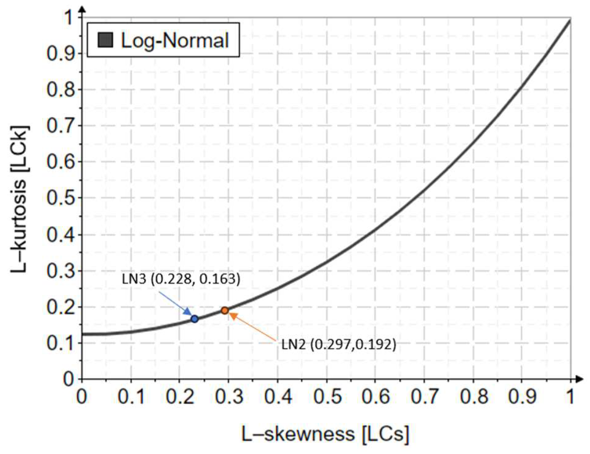
Appendix F. A Comparative Analysis of the Log-Normal Distribution
References
- Elsebaie, I. Developing rainfall intensity–duration–frequency relationship for two regions in Saudi Arabia. J. King Saud Univ.-Eng. Sci. 2012, 24, 131–140. [Google Scholar] [CrossRef]
- Ewea, H.A.; Elfeki, A.M.; Al-Amri, N.S. Al-Amri Development of intensity–duration–frequency curves for the Kingdom of Saudi Arabia. Geomat. Nat. Hazards Risk 2017, 8, 570–584. [Google Scholar] [CrossRef]
- Agarwal, S.; Kumar, S.; Singh, U.K. Intensity Duration Frequency Curve Generation using Historical and Future Downscaled Rainfall Data. Indian J. Ecol. 2021, 48, 275–280. [Google Scholar]
- Palaka, R.; Prajwala, G.; Navyasri, K.V.S.N.; Anish, I. Development of intensity duration frequency curves for narsapur mandal, telangana state, India. Int. J. Res. Eng. Technol. 2016, 5, 109–113. [Google Scholar]
- Kawara, A.Q.; Elsebaie, I.H. Development of Rainfall Intensity, Duration and Frequency Relationship on a Daily and Sub-Daily Basis (Case Study: Yalamlam Area, Saudi Arabia). Water 2022, 14, 897. [Google Scholar] [CrossRef]
- Markiewicz, I. Depth–Duration–Frequency Relationship Model of Extreme Precipitation in Flood Risk Assessment in the Upper Vistula Basin. Water 2021, 13, 3439. [Google Scholar] [CrossRef]
- Gumbel, E.J. Statistical theory of floods and droughts. J. Inst. Water Eng. 1958, 12, 157–184. [Google Scholar]
- Subah, Z.; Bala, S.K.; Ryu, J.H. Assessing Urban Flooding Extent of the Baunia Khal Watershed in Dhaka, Bangladesh. Water 2023, 15, 1183. [Google Scholar] [CrossRef]
- Vangelis, H.; Zotou, I.; Kourtis, I.M.; Bellos, V.; Tsihrintzis, V.A. Relationship of Rainfall and Flood Return Periods through Hydrologic and Hydraulic Modeling. Water 2022, 14, 3618. [Google Scholar] [CrossRef]
- Hydrology Subcommittee; Interagency Advisory Committee on Water Data; U.S. Department of the Interior; U.S. Geological Survey; Office of Water Data Coordination. Bulletin 17B Guidelines for Determining Flood Flow Frequency; Hydrology Subcommittee, Interagency Advisory Committee on Water Data, U.S. Department of the Interior, U.S. Geological Survey, Office of Water Data Coordination: Reston, VA, USA, 1981.
- U.S. Department of the Interior; U.S. Geological Survey. Bulletin 17C Guidelines for Determining Flood Flow Frequency; U.S. Department of the Interior, U.S. Geological Survey: Reston, VA, USA, 2017.
- Dhakal, S.; Bhattarai, U.; Marahatta, S.; Devkota, P. Impact of climate change on the full spectrum of future low flows of Budhigandaki River Basin in Nepal using Gumbel distribution. Int. J. Energy Water Res. 2023, 7, 191–203. [Google Scholar] [CrossRef]
- Langat, P.K.; Kumar, L.; Koech, R. Identification of the Most Suitable Probability Distribution Models for Maximum, Minimum, and Mean Streamflow. Water 2019, 11, 734. [Google Scholar] [CrossRef]
- Balacco, G.; Carbonara, A.; Gioia, A.; Iacobellis, V.; Piccinni, A.F. Evaluation of Peak Water Demand Factors in Puglia (Southern Italy). Water 2017, 9, 96. [Google Scholar] [CrossRef]
- Sun, P.; Zhang, Q.; Yao, R.; Singh, V.P.; Song, C. Low Flow Regimes of the Tarim River Basin, China: Probabilistic Behavior, Causes and Implications. Water 2018, 10, 470. [Google Scholar] [CrossRef]
- Gray, D.M. Synthetic hydrographs for small drainage areas. J. Hydraul. Div. ASCE 1961, 87 HY4, 33–54. [Google Scholar] [CrossRef]
- Haktanir, T.; Nurullah, S. Suitability of two-parameter gamma distribution and three-parameter beta distribution as synthetic hydrographs in Anatolia. Hydrol. Sci. J. 1990, 35, 167–184. [Google Scholar] [CrossRef]
- Croley, T.E. Gamma synthetic hydrographs. J. Amst. Hydrol. 1980, 47, 41–52. [Google Scholar] [CrossRef]
- Bhunya, P.K.; Berndtsson, R.; Ojha, C.S.P.; Mishra, S.K. Suitability of Gamma, Chi-square, Weibull and Beta distributions as synthetic unit hydrographs. J. Hydrol. 2007, 334, 28–38. [Google Scholar] [CrossRef]
- Bhunya, P.K.; Berndtsson, R.; Singh, P.K.; Hubert, P. Comparison between Weibull and gamma distributions to derive synthetic unit hydrograph using Horton ratios. Water Resour. 2008, 44, WR006031. [Google Scholar] [CrossRef]
- Bhunya, P. Synthetic Unit Hydrograph Methods: A Critical Review. Open Hydrol. J. 2011, 5, 1–8. [Google Scholar] [CrossRef]
- Rao, A.R.; Hamed, K.H. Flood Frequency Analysis; CRC Press LLC.: Boca Raton, FL, USA, 2000. [Google Scholar]
- Singh, V.P. Entropy-Based Parameter Estimation in Hydrology; Springer: Dordrecht, The Netherlands, 1998. [Google Scholar]
- World Meteorological Organization. (WMO-No.718) 1989 Statistical Distributions for Flood Frequency Analysis; Operational Hydrology Report no. 33; WHO: Geneva, Switzerland, 1989. [Google Scholar]
- Singh, V.P.; Guo, H. Parameter estimation for 2-parameter log-logistic distribution (LLD2) by maximum entropy. Civ. Eng. Syst. 1995, 12, 343–357. [Google Scholar] [CrossRef]
- Shoukri, M.M.; Mian, I.U.H.; Tracy, D.S. Sampling properties of estimators of the log-logistic distribution with application to Canadian precipitation data. Can. J. Stat. Rev. Can. Stat. 1988, 16, 223–236. [Google Scholar] [CrossRef]
- Fitzgerald, D.L. Analysis of extreme rainfall using the log logistic distribution. Stoch. Environ. Res. Risk Assess. 2005, 19, 249–257. [Google Scholar] [CrossRef]
- Hussain, Z. Rainfall frequency analysis using frechet and log-logistic distributions of sites of azad jammu and kashmir, pakistan. Appl. Ecol. Environ. Res. 2019, 17, 13607–13623. [Google Scholar] [CrossRef]
- Ahmad, M.I.; Sinclair, C.D.; Werritti, A. Log-logistic flood frequency analysis. J. Hydrol. 1988, 98, 205–224. [Google Scholar] [CrossRef]
- Haktanir, T. Statistical modeling of annual maximum flows in Turkish rivers. Hydrol. Sci. J. 1991, 36, 367–389. [Google Scholar] [CrossRef]
- Ahilan, S.; Bruen, M.; O’Sullivan, J.J. Influences on flood frequency distributions in Irish river catchments. Hydrol. Earth Syst. Sci. 2012, 16, 1137–1150. [Google Scholar] [CrossRef]
- Tegegne, G.; Melesse, A.M.; Asfaw, D.H.; Worqlul, A.W. Flood Frequency Analyses over Different Basin Scales in the Blue Nile River Basin, Ethiopia. Hydrology 2020, 7, 44. [Google Scholar] [CrossRef]
- Anghel, C.G.; Ilinca, C. Parameter Estimation for Some Probability Distributions Used in Hydrology. Appl. Sci. 2022, 12, 12588. [Google Scholar] [CrossRef]
- Hosking, J.R.M.; Wallis, J.R. Regional Frequency Analysis: An Approach Based on L–Moments; Cambridge University Press: Cambridge, UK, 1997. [Google Scholar]
- De Luca, D.L.; Napolitano, F. A user-friendly software for modelling extreme values: EXTRASTAR (extremes abacus for statistical regionalization). Environ. Model. Softw. 2023, 161, 105622. [Google Scholar] [CrossRef]
- Alem, A.M.; Tilahun, S.A.; Moges, M.A.; Melesse, A.M. A Regional Hourly Maximum Rainfall Extraction Method for Part of Upper Blue Nile Basin, Ethiopia; Elsevier Inc.: Amsterdam, The Netherlands, 2019. [Google Scholar] [CrossRef]
- Lin, G.F.; Chen, L.H. Identification of Homogeneous Regions for Regional Frequency Analysis Using the Self-Organizing Map. J. Hydrol. 2006, 324, 1–9. [Google Scholar] [CrossRef]
- Rao, A.R.; Srinivas, V.V. Introduction. In Regionalization of Watersheds: An Approach Based on Cluster Analysis; Rao, A.R., Srinivas, V.V., Eds.; Springer: Dordrecht, The Netherlands, 2008; pp. 1–16. [Google Scholar]
- Yin, Y.; Chen, H.; Xu, C.Y.; Xu, W.; Chen, C.; Sun, S. Spatio-Temporal Characteristics of the Extreme Precipitation by L-Moment-Based Index-Flood Method in the Yangtze River Delta Region. China Theor. Appl. Climatol. 2016, 124, 1005–1022. [Google Scholar] [CrossRef]
- Cassalho, F.; Beskow, S.; de Mello, C.R.; de Moura, M.M.; de Oliveira, L.F.; de Aguiar, M.S. Artificial intelligence for identifying hydrologically homogeneous regions: A state-of-the-art regional flood frequency analysis. Hydrol. Process. 2019, 33, 1101–1116. [Google Scholar] [CrossRef]
- Stedinger, J.R.; Tasker, G.D. Regional hydrologic analysis: 1. Ordinary, weighted, and generalized least squares compared. Water Resour. Res. 1985, 21, 1421–1432. [Google Scholar] [CrossRef]
- Griffis, V.W.; Stedinger, J.R. The use of GLS regression in regional hydrologic analyses. J. Hydrol. 2007, 344, 82–95. [Google Scholar] [CrossRef]
- Borga, M.; Vezzani, C.; Fontana, G.D. Regional Rainfall Depth–Duration–Frequency Equations for an Alpine Region. Nat. Hazards 2005, 36, 221–235. [Google Scholar] [CrossRef]
- Libertino, A.; Allamano, P.; Laio, F.; Claps, P. Regional-scale analysis of extreme precipitation from short and fragmented records. Adv. Water Resour. 2018, 112, 147–159. [Google Scholar] [CrossRef]
- Chokmani, K.; Ouarda, T.B.M.J. Physiographical space-based kriging for regional flood frequency estimation at ungauged sites. Water Resour. Res. 2004, 40, W1251. [Google Scholar] [CrossRef]
- Chebana, F.; Ouarda, T.B.M.J. Depth and homogeneity in regional flood frequency analysis. Water Resour. Res. 2008, 44, W11422. [Google Scholar] [CrossRef]
- Skoien, J.; Merz, R.; Bloschl, G. Top-kriging—Geostatistics on stream networks. Hydrol. Earth Syst. Sci. 2006, 10, 277–287. [Google Scholar] [CrossRef]
- Ministry of Regional Development and Tourism. The Regulations Regarding the Establishment of Maximum Flows and Volumes for the Calculation of Hydrotechnical Retention Constructions; Indicative NP 129–2011; Ministry of Regional Development and Tourism: Bucharest, Romania, 2012.
- Diacon, C.; Serban, P. Hydrological Syntheses and Regionalizations; Technical Publishing House: Bucharest, Romania, 1994. [Google Scholar]
- Houghton, C. Birth of a Parent: The Wakeby Distribution for Modeling Flood Flows; Working Paper no. MIT-EL77–033WP; Water Resources Research: Tucson, AZ, USA, 1978; Volume 14. [Google Scholar]
- Murshed, S.; Park, B.-J.; Jeong, B.-Y.; Park, J.-S. LH-Moments of Some Distributions Useful in Hydrology. Commun. Stat. Appl. Methods 2009, 16, 647–658. [Google Scholar] [CrossRef]
- Rameshwar, D.G.; Kundu, D. Generalized exponential distribution: Different method of estimations. J. Stat. Comput. Simul. 2001, 69, 315–337. [Google Scholar]
- Crooks, G.E. Field Guide to Continuous Probability Distributions; Berkeley Institute for Theoretical Science: Berkeley, CA, USA, 2019. [Google Scholar]
- Wang, Q.J. LH moments for statistical analysis of extreme events. Water Resour. Res. 1997, 33, 2841–2848. [Google Scholar] [CrossRef]
- Chow, V.T.; Maidment, D.R.; Mays, L.W. Applied Hydrology; McGraw-Hill, Inc.: New York, NY, USA, 1988; ISBN 007-010810-2. [Google Scholar]
- World Meteorological Organization. (WMO-No.233) Estimation of Maximum Floods; Technical Note no. 98; WHO: Geneva, Switzerland, 1969. [Google Scholar]
- Grimaldi, S.; Kao, S.-C.; Castellarin, A.; Papalexiou, S.-M.; Viglione, A.; Laio, F.; Aksoy, H.; Gedikli, A. Statistical Hydrology. In Treatise on Water Science; Elsevier: Oxford, UK, 2011; Volume 2, pp. 479–517. [Google Scholar]
- Department of the Army; U.S. Army Corps of Engineers. EM 1110–2-1415 Hydrologic Frequency Analysis, Engineering and Design; Department of the Army, U.S. Army Corps of Engineers: Washington, DC, USA, 1993.
- Ministry of the Environment. The Romanian Water Classification Atlas, Part I—Morpho-Hydrographic Data on the Surface Hydrographic Network; Ministry of the Environment: Bucharest, Romania, 1992.
- Obreja, F. The Study of Sediment Yield in the Siret River Basin. Ph.D. Thesis, Stefan the Great University, Suceava, Romania, 2013. [Google Scholar]
- Vanmaercke, M.; Obreja, F.; Poesen, J. Seismic controls on contemporary sediment export in the Siret river catchment, Romania. Geomorphology 2014, 216, 247–262. [Google Scholar] [CrossRef]
- Zavoianu, I. Hydrology; Romania de Maine Publishing House: Bucharest, Romania, 2006. [Google Scholar]
- Lang, M.; Ouarda, T.B.; Bobée, B. Towards operational guidelines for over-threshold modeling. J. Hydrol. 1999, 225, 103–117. [Google Scholar] [CrossRef]
- Anghel, C.G.; Ilinca, C. Evaluation of Various Generalized Pareto Probability Distributions for Flood Frequency Analysis. Water 2023, 15, 1557. [Google Scholar] [CrossRef]
- Machiwal, D.; Jha, M.K. Stochastic Modelling of Time Series. In Hydrologic Time Series Analysis: Theory and Practice; Machiwal, D., Jha, M.K., Eds.; Springer: Dordrecht, The Netherlands, 2012; pp. 85–95. [Google Scholar] [CrossRef]
- Strupczewski, W.G.; Kochanek, K.; Bogdanowicz, E. Flood frequency analysis supported by the largest historical flood. Nat. Hazards Earth Syst. Sci. 2014, 14, 1543–1551. [Google Scholar] [CrossRef]
- Benaini, M.; Achite, M.; Amin, M.G.M.; Singh, V.P. Frequency analysis of annual maximum daily precipitation in northeastern Algeria: Mapping and implications under climate variability. Theor. Appl. Climatol. 2023, 153, 1411–1424. [Google Scholar] [CrossRef]
- Anghel, C.G.; Ilinca, C. Predicting Flood Frequency with the LH-Moments Method: A Case Study of Prigor River, Romania. Water 2023, 15, 2077. [Google Scholar] [CrossRef]
- Ilinca, C.; Anghel, C.G. Frequency Analysis of Extreme Events Using the Univariate Beta Family Probability Distributions. Appl. Sci. 2023, 13, 4640. [Google Scholar] [CrossRef]
- Rao, G.S.; Albassam, M.; Aslam, M. Evaluation of Bootstrap Confidence Intervals Using a New Non-Normal Process Capability Index. Symmetry 2019, 11, 484. [Google Scholar] [CrossRef]
- Beaumont, J.-F.; Émond, N. A Bootstrap Variance Estimation Method for Multistage Sampling and Two-Phase Sampling When Poisson Sampling Is Used at the Second Phase. Stats 2022, 5, 339–357. [Google Scholar] [CrossRef]
- Bochniak, A.; Kluza, P.A.; Kuna-Broniowska, I.; Koszel, M. Application of Non-Parametric Bootstrap Confidence Intervals for Evaluation of the Expected Value of the Droplet Stain Diameter Following the Spraying Process. Sustainability 2019, 11, 7037. [Google Scholar] [CrossRef]
- Markiewicz, I.; Bogdanowicz, E.; Kochanek, K. On the Uncertainty and Changeability of the Estimates of Seasonal Maximum Flows. Water 2020, 12, 704. [Google Scholar] [CrossRef]
- Markiewicz, I.; Bogdanowicz, E.; Kochanek, K. Quantile Mixture and Probability Mixture Models in a Multi-Model Approach to Flood Frequency Analysis. Water 2020, 12, 2851. [Google Scholar] [CrossRef]
- Kochanek, K.; Strupczewski, W.G.; Bogdanowicz, E.; Markiewicz, I. The bias of the maximum likelihood estimates of flood quantiles based solely on the largest historical records. J. Hydrol. 2020, 584, 124740. [Google Scholar] [CrossRef]
- Drobot, R.; Draghia, A.F.; Chendes, V.; Sirbu, N.; Dinu, C. Consideratii privind viiturile sintetice pe Dunare. Hidrotehnica 2023, 68. (In Romanian) [Google Scholar]


| New Elements | Distribution |
|---|---|
| Exact relationships for estimating parameters for LH-moments | G, Γ2,LN2,L2,LL2,W2,F2, E2,EG,R2,PV2,CH2, ICH2 |
| Approximate relations for estimating parameters for LH-moments | Γ2,LN2, PV2,CH2, ICH2 |
| Approximate relations for estimating parameters for L-moments | LN2,CH2, ICH2 |
| Diagrams and relationships of | G, Γ2,LN2,L2,LL2,W2,F2, E2,EG,R2,PV2,CH2, ICH2 |
| Diagrams and relationships of | G, Γ2,LN2,L2,LL2,W2,F2, E2,EG,R2,PV2,CH2, ICH2 |
| Distr. | |||
|---|---|---|---|
| PV2 | |||
| CH2 | |||
| ICH2 | |||
| Γ2 | |||
| LN2 | |||
| G | |||
| L2 | |||
| LL2 | |||
| E2 | |||
| R2 | |||
| W2 | |||
| F2 | |||
| EG |
| Year | 1970 | 1971 | 1972 | 1973 | 1974 | 1975 | 1976 | 1977 | 1978 | 1979 | 1980 | |
| Flow | [m3/s] | 3186 | 1966 | 1842 | 1535 | 1260 | 1860 | 630 | 889 | 1320 | 1280 | 989 |
| Year | 1981 | 1982 | 1983 | 1984 | 1985 | 1986 | 1987 | 1988 | 1989 | 1990 | 1991 | |
| Flow | [m3/s] | 2040 | 901 | 1420 | 2460 | 1400 | 334 | 275 | 2620 | 1370 | 275 | 3270 |
| Year | 1992 | 1993 | 1994 | 1995 | 1996 | 1997 | 1998 | 1999 | 2000 | 2001 | 2002 | |
| Flow | [m3/s] | 2045 | 1020 | 604 | 1120 | 1612 | 1040 | 1380 | 830 | 447 | 435 | 2200 |
| Year | 2003 | 2004 | 2005 | 2006 | 2007 | 2008 | ||||||
| Flow | [m3/s] | 796 | 727 | 4650 | 1375 | 785 | 2068 | |||||
| Siret River, Lungoci Station, Romania | Central Moments and Indicators | ||||||
| MOM | |||||||
| [m3/s] | [m3/s] | [−] | [−] | [−] | |||
| 1443 | 915 | 0.634 | 1.413 | 5.872 | |||
| L-Moments | |||||||
| [m3/s] | [m3/s] | [m3/s] | [m3/s] | [−] | [−] | [−] | |
| 1443 | 490 | 112 | 90.6 | 0.339 | 0.228 | 0.185 | |
| LH-Moments (First Level) | |||||||
| [m3/s] | [m3/s] | [m3/s] | [m3/s] | [−] | [−] | [−] | |
| 1932 | 451 | 135 | 89.9 | 0.233 | 0.299 | 0.199 | |
| LH-Moments (Second Level) | |||||||
| [m3/s] | [m3/s] | [m3/s] | [m3/s] | [−] | [−] | [−] | |
| 2233 | 442 | 148 | 90.7 | 0.198 | 0.334 | 0.205 | |
| Distr. | Methods | |||||||||||||
|---|---|---|---|---|---|---|---|---|---|---|---|---|---|---|
| MOM | L-Moments | LH-Moments (First Level) | LH-Moments (Second Level) | |||||||||||
| RME | RAE | RME | RAE | RME | RAE | RME | RAE | |||||||
| PV2 | 0.047 | 0.162 | 0.034 | 0.132 | 0.385 | 0.263 | 0.047 | 0.155 | 0.382 | 0.233 | 0.054 | 0.178 | 0.384 | 0.225 |
| CH2 | 0.026 | 0.104 | 0.022 | 0.083 | 0.143 | 0.101 | 0.031 | 0.130 | 0.199 | 0.105 | 0.041 | 0.178 | 0.227 | 0.110 |
| ICH2 | 0.065 | 0.228 | 0.045 | 0.179 | 0.453 | 0.323 | 0.063 | 0.211 | 0.426 | 0.272 | 0.073 | 0.241 | 0.418 | 0.255 |
| Γ2 | 0.013 | 0.058 | 0.013 | 0.058 | 0.209 | 0.137 | 0.014 | 0.062 | 0.257 | 0.140 | 0.017 | 0.075 | 0.280 | 0.144 |
| LN2 | 0.025 | 0.085 | 0.019 | 0.077 | 0.297 | 0.192 | 0.025 | 0.085 | 0.323 | 0.185 | 0.027 | 0.093 | 0.336 | 0.185 |
| G | 0.030 | 0.079 | 0.028 | 0.074 | 0.170 | 0.150 | 0.041 | 0.114 | 0.243 | 0.147 | 0.053 | 0.162 | 0.272 | 0.149 |
| L2 | 0.108 | 0.254 | 0.100 | 0.238 | 0.000 | 0.167 | 0.178 | 0.085 | 0.148 | 0.139 | 0.229 | 0.085 | 0.208 | 0.137 |
| LL2 | 0.038 | 0.146 | 0.022 | 0.086 | 0.339 | 0.263 | 0.031 | 0.114 | 0.379 | 0.251 | 0.038 | 0.140 | 0.394 | 0.246 |
| E2 | 0.045 | 0.143 | 0.036 | 0.132 | 0.333 | 0.167 | 0.054 | 0.157 | 0.333 | 0.167 | 0.038 | 0.175 | 0.333 | 0.167 |
| R2 | 0.043 | 0.140 | 0.033 | 0.108 | 0.114 | 0.105 | 0.063 | 0.207 | 0.175 | 0.105 | 0.097 | 0.324 | 0.205 | 0.109 |
| W2 | 0.021 | 0.084 | 0.019 | 0.072 | 0.162 | 0.111 | 0.023 | 0.099 | 0.222 | 0.119 | 0.029 | 0.129 | 0.253 | 0.127 |
| F2 | 0.078 | 0.275 | 0.049 | 0.193 | 0.471 | 0.340 | 0.072 | 0.243 | 0.450 | 0.293 | 0.087 | 0.287 | 0.441 | 0.275 |
| EG | 0.013 | 0.059 | 0.013 | 0.060 | 0.231 | 0.151 | 0.013 | 0.060 | 0.275 | 0.152 | 0.013 | 0.063 | 0.295 | 0.155 |
| Relative Errors [%] | |||||||
|---|---|---|---|---|---|---|---|
| Elements | Length (n) | Length (n) | |||||
| 1000 | 80 | 50 | 25 | 80 | 50 | 25 | |
| 1 | 0.994 | 0.991 | 0.985 | 0.6 | 0.9 | 1.5 | |
| 1 | 0.933 | 0.914 | 0.878 | 6.7 | 8.6 | 12.2 | |
| 4 | 3.61 | 3.51 | 3.31 | 9.75 | 12.25 | 17.25 | |
| 41 | 32.8 | 30.81 | 27.36 | 20 | 24.85 | 33.27 | |
| 0.833 | 0.791 | 0.779 | 0.756 | 5.04 | 6.48 | 9.24 | |
| −0.347 | −0.319 | −0.313 | −0.301 | 8.78 | 10.86 | 15.28 | |
| 15.6 | 13.8 | 13.3 | 12.3 | 11.9 | 15.2 | 21.3 | |
| 9.27 | 8.38 | 8.13 | 7.65 | 9.58 | 12.3 | 12.3 | |
| 6.04 | 5.58 | 5.44 | 5.19 | 7.64 | 9.84 | 9.84 | |
| 4.91 | 4.58 | 4.48 | 4.30 | 6.69 | 8.64 | 12.4 | |
| 1 | 0.969 | 0.957 | 0.933 | 3.1 | 4.3 | 6.7 | |
| 2 | 1.602 | 1.532 | 1.417 | 19.9 | 23.4 | 58.3 | |
| 14 | 8.92 | 8.2 | 6.73 | 32.3 | 41.56 | 51.91 | |
| 947 | 287.5 | 231.4 | 140.6 | 69.64 | 75.56 | 85.15 | |
| 1.269 | 1.128 | 1.099 | 1.049 | 11.11 | 13.4 | 17.34 | |
| −0.805 | −0.667 | −0.648 | −0.62 | 20.69 | 24.23 | 29.84 | |
| 50.1 | 34.0 | 31.2 | 26.6 | 32.1 | 37.7 | 32.1 | |
| 22.6 | 16.7 | 15.6 | 13.8 | 25.8 | 30.7 | 30.7 | |
| 11.7 | 9.4 | 8.9 | 8.0 | 20.2 | 24.4 | 24.4 | |
| 8.6 | 7.1 | 6.8 | 6.2 | 17.4 | 21.1 | 27.8 | |
| Relative Errors [%] | |||||||
|---|---|---|---|---|---|---|---|
| Elements | Length (n) | Length (n) | |||||
| 1000 | 80 | 50 | 25 | 80 | 50 | 25 | |
| 1 | 0.999 | 0.999 | 0.999 | 0.1 | 0.1 | 0.1 | |
| 0.3 | 0.3 | 0.3 | 0.3 | 0 | 0 | 0 | |
| 0.2618 | 0.263 | 0.2638 | 0.2659 | 0.46 | 0.76 | 1.55 | |
| 0.1767 | 0.1775 | 0.1782 | 0.1803 | 0.45 | 0.85 | 2.04 | |
| 0.545 | 0.544 | 0.544 | 0.544 | 0.18 | 0.18 | 0.18 | |
| −0.148 | −0.149 | −0.149 | −0.150 | 0.67 | 0.67 | 1.33 | |
| 6.54 | 6.52 | 6.53 | 6.54 | 0.18 | 0.15 | 0.08 | |
| 4.64 | 4.63 | 4.64 | 4.64 | 0.17 | 0.13 | 0.02 | |
| 3.51 | 3.50 | 3.50 | 3.51 | 0.14 | 0.11 | 0 | |
| 3.06 | 3.06 | 3.06 | 3.06 | 0.13 | 0.1 | 0 | |
| 1 | 0.989 | 0.985 | 0.975 | 1.1 | 1.5 | 2.5 | |
| 0.5 | 0.495 | 0.494 | 0.493 | 1 | 1.2 | 0.7 | |
| 0.4404 | 0.4359 | 0.4349 | 0.4337 | 1.03 | 1.25 | 1.52 | |
| 0.277 | 0.274 | 0.2717 | 0.2714 | 1.08 | 1.91 | 2.02 | |
| 0.947 | 0.935 | 0.934 | 0.933 | 1.27 | 1.37 | 1.48 | |
| −0.448 | −0.448 | −0.452 | −0.460 | 0 | 0.89 | 2.68 | |
| 21.6 | 20.7 | 20.5 | 20.3 | 4.23 | 5.94 | 6.18 | |
| 11.9 | 11.5 | 11.4 | 11.3 | 3.52 | 4.18 | 5.35 | |
| 7.32 | 7.11 | 7.06 | 6.98 | 2.94 | 3.54 | 4.67 | |
| 5.78 | 5.63 | 5.59 | 5.53 | 2.66 | 3.23 | 4.36 | |
| Elements | Length (n) | Relative Errors [%] | |
|---|---|---|---|
| 1000 | 39 | ||
| (MOM) | |||
| 1442 | 1440 | 0.14 | |
| 0.634 | 0.603 | 4.89 | |
| 2.157 | 2.027 | 6.03 | |
| 12.27 | 11.1 | 9.54 | |
| 0.581 | 0.557 | 4.13 | |
| 7.105 | 7.117 | 0.17 | |
| 10,579 | 9776 | 7.59 | |
| 7340 | 6889 | 6.14 | |
| 5443 | 5173 | 4.96 | |
| 4708 | 4502 | 4.38 | |
| (L-moments) | |||
| 1442 | 1438 | 0.28 | |
| 0.339 | 0.339 | 0 | |
| 0.2964 | 0.2976 | 0.41 | |
| 0.192 | 0.1934 | 0.73 | |
| 0.62 | 0.619 | 0.16 | |
| 7.082 | 7.08 | 0.03 | |
| 11,923 | 11,859 | 0.54 | |
| 8075 | 8037 | 0.47 | |
| 5871 | 5846 | 0.43 | |
| 5030 | 5010 | 0.4 | |
Disclaimer/Publisher’s Note: The statements, opinions and data contained in all publications are solely those of the individual author(s) and contributor(s) and not of MDPI and/or the editor(s). MDPI and/or the editor(s) disclaim responsibility for any injury to people or property resulting from any ideas, methods, instructions or products referred to in the content. |
© 2023 by the authors. Licensee MDPI, Basel, Switzerland. This article is an open access article distributed under the terms and conditions of the Creative Commons Attribution (CC BY) license (https://creativecommons.org/licenses/by/4.0/).
Share and Cite
Anghel, C.G.; Stanca, S.C.; Ilinca, C. Two-Parameter Probability Distributions: Methods, Techniques and Comparative Analysis. Water 2023, 15, 3435. https://doi.org/10.3390/w15193435
Anghel CG, Stanca SC, Ilinca C. Two-Parameter Probability Distributions: Methods, Techniques and Comparative Analysis. Water. 2023; 15(19):3435. https://doi.org/10.3390/w15193435
Chicago/Turabian StyleAnghel, Cristian Gabriel, Stefan Ciprian Stanca, and Cornel Ilinca. 2023. "Two-Parameter Probability Distributions: Methods, Techniques and Comparative Analysis" Water 15, no. 19: 3435. https://doi.org/10.3390/w15193435
APA StyleAnghel, C. G., Stanca, S. C., & Ilinca, C. (2023). Two-Parameter Probability Distributions: Methods, Techniques and Comparative Analysis. Water, 15(19), 3435. https://doi.org/10.3390/w15193435