Article

Effect of Flume Width on the Hydraulic Properties of Overland Flow from Laboratory Observation

Jinshan Soil and Water Conservation Research Center, Fujian Agriculture and Forestry University, Fuzhou 350002, China
*
Author to whom correspondence should be addressed.
Water 2023, 15(19), 3416; https://doi.org/10.3390/w15193416
Submission received: 15 August 2023 / Revised: 23 September 2023 / Accepted: 24 September 2023 / Published: 28 September 2023
(This article belongs to the Section Hydraulics and Hydrodynamics)

Abstract

:
The effect of flume width (b) on overland flow dynamics was investigated in this study. Experiments were conducted with five different flow discharges and five flume widths (0.05–0.30 m, with an interval of 0.05 m). The findings revealed that a narrow flume had a noticeable impact on flow acceleration as the slope length increased. Relative average deviation (RAD) was calculated to evaluate the influence of sidewall effects on flow velocity. The coefficient of variation in the RAD ranged from 1.90% to 3.65%. The RAD has extremely significant differences between different widths when the flow is 0.02–0.08 m2/min. The significant differences in the RAD at different widths decrease as the flow rate increases. The flow regime was evaluated using the ratio of the thickness of the viscous sublayer to the water depth (δ/h), which proved to be a better indicator than the Reynolds number for studying flow regimes in different flume widths. Furthermore, it was observed that the energy variation was smaller in narrow flumes (b = 0.5–0.10 m) compared to wider flumes (b = 0.25–0.30 m). When the flume width ranged from 0.15 to 0.30 m, the specific energy change increased. These results contribute to further understanding of the hydraulic characteristics of overland flow and provide theoretical references for optimizing experimental design.

1. Introduction

Overland flow is a shallow open flow moving on the ground surface along a slope under gravity control. Overland flow is the initial stage of soil detachment and ultimately results in soil erosion. The depth of overland flow is very shallow, i.e., generally less than a few millimeters, and thus is unstable. The characteristics of overland flow dynamics are influenced by many conditions, including rainfall, slope gradient, soil properties, underlying surface characteristics, land use patterns, topographic features and anthropogenic factors. A comprehensive understanding of the influence of these conditions on the hydrodynamics of overland flow is crucial for exploring soil erosion mechanisms and hydrologic processes. Thus, numerous laboratory simulation experiments have been designed to study these factors. The scour simulation method has been widely used in laboratory simulations [1,2,3,4,5,6,7]. Laboratory-simulated experiments were conducted under different conditions to measure the effects of specific conditions on runoff, sediment yield and soil erosion processes.
The study of overland flow properties is mainly based on kinetic characteristic analysis. Currently, the kinetic analysis of overland flow includes the following aspects: research on the measurement of flow velocity and water depth (kinetic indicators), studies on the flow patterns of overland flow and the influence of different underlying surface characteristics on overland flow. The calculations of overland flow hydraulics are derived from flow velocity and water depth measurements. Flow velocity and water depth are mainly influenced by external factors such as rainfall, slope gradient, roughness and boundary conditions [8,9,10,11]. Unlike open channel flow, the changes in velocity and depth of overland flow are unstable. Dye tracing is the most commonly used method for field and laboratory measurements of overland flow velocities [12,13]. Xia et al. [14] developed an electrolyte pulse technique for measuring overland flow velocities, which is similar in principle to salt tracer methods [15]. Many researchers have started using instruments based on noncontact optoelectronic principles to measure overland flow velocities. Li [16], Wang et al. [17] and Bai et al. [18] constructed overland flow velocity measurement systems based on infrared optoelectronic sensors. Yang et al. [19] used a PIV velocimeter to investigate the flow structure of overland flow when studying its hydraulic characteristics. Common water depth measurement methods can be divided into two categories: direct measurement and indirect measurement. Direct measurement methods usually use tools such as rulers, cursor calipers and depth gauges. These tools make the measurement process relatively direct and simple. Another method is indirect measurement, which calculates average water depth using measured mean discharge and mean velocity along with hydraulic equations [20]. This method does not require direct measurement of water depth but instead derives depth values indirectly through parameters such as discharge and velocity. Zhu et al. [21] conducted detailed analysis of overland flow depth variations using laser edge detection algorithms. However, the effectiveness of certain measurement techniques may be constrained when applied outside of optimal conditions.
There is still no agreement on categorizing flow patterns of overland flow, primarily due to its high instability and sensitivity to various influencing factors. This makes the definitive classification as laminar, turbulent, transitional or mixed flow challenging. Horton [22] quantitatively studied the flow regimes of overland flow by describing soil infiltration processes and surface ponding phenomena and believed that overland flow was a completely turbulent flow interspersed with laminar flow. Emmett [15] found through experimental observations that overland flow was different from the definitions of laminar, transitional and turbulent flows in open channel flow. Overland flow had very intense disturbances and exhibited characteristics of both turbulent and laminar flows, which he termed “disturbed flow”. Sha and Jiang [23] found that overland flow patterns are highly responsive to slope changes, transitioning from subcritical to supercritical flow regimes as slope gradients increase. Additionally, Zhang et al. [24] identified that based on critical unit discharges, overland flow is rarely present in subcritical zones, instead occurring in a wavy, slow-moving mode at low discharges, while forming rolling waves under high, rapid flows.
The underlying surface condition includes the resistance, cross-sectional area and cross-sectional shape. The overland flow resistance is a significant parameter controlling the hydrodynamics. Current studies on the underlying surface conditions of overland flow have mainly concentrated on resistance. Traditional hydraulic methods for calculating friction factors have been used to study overland flow roughness in previous studies, such as Darcy–Weisbach’s, Manning’s or Chezy’s coefficients [25,26]. The total resistance to overland flow has traditionally been divided into several parts [13]. These parts contain grain, form, wave and rain resistance [27,28,29]. It is widely believed that the relationship between roughness and Reynolds number can characterize grain resistance. Ma et al. [30] indicated that grain resistance is related to water depth and Reynolds number. This may be due to the water depth of overland flow being too shallow and extremely sensitive to the change in roughness [31,32]. The resistance caused by vegetation obstructing the overland flow is form resistance. Much research has been conducted on the influencing factors of vegetation on form resistance. These factors include types, density, attributes (flexibility and rigidity) and coverage [8,10,33,34,35]. In previous studies, there was no consensus on the effect of rainfall on resistance (increasing or decreasing resistance) [36,37]. Research on wave resistance is relatively rare. Noarayanan et al. [29] indicated that the total resistance equals the sum of these four resistance items, which they accord with a sum law. The “superposition principle” of resistance is the focus of current research [7,30,38].
The flume width influences the area and shape of the cross-section as well as the hydraulic radius, which is an important indicator for calculating the hydraulic parameters of overland flow. However, there has been limited research on the effect of flume width on the hydraulic characteristics of overland flow, despite the important influence of flume width on the hydraulic radius. The discussion of the relationship between the flume width and overland flow has concentrated on the effect of the flume width on soil erosion. The flume width influences the sediment transport, runoff rate and feasibility of the soil erosion model [16,39,40]. Flume widths are usually selected based on experimental conditions when studying overland flow movement. For indoor simulated flume experiments, flume widths are often between 0.1 and 1.0 m. These studies utilize flumes of different widths as presented in Table 1, but there are no clear criteria for selecting flume width [1,4,5,37,41,42,43,44,45,46]. Whether the choice of flume width affects velocity measurements and thus influences the hydraulics of overland flow in actual experiments has not been reported. Therefore, exploring the relationship between flume width and overland flow is a very critical issue in this study.
Therefore, the objectives of this study were to judge the effect of the flume width on flow velocity measurements, investigate the flow pattern of overland flow under different flume widths, and ascertain the effect of the flume width on the specific energy and clarify the main reason for the effect. Hydraulic characteristics have a significant effect on soil erosion. This study can provide a theoretical foundation for studying the relationship between the flume width and hydraulic characteristics of overland flow in order to further understand the hydraulic characteristics of overland flow and provide theoretical references for optimizing experimental design.

2. Materials and Methods

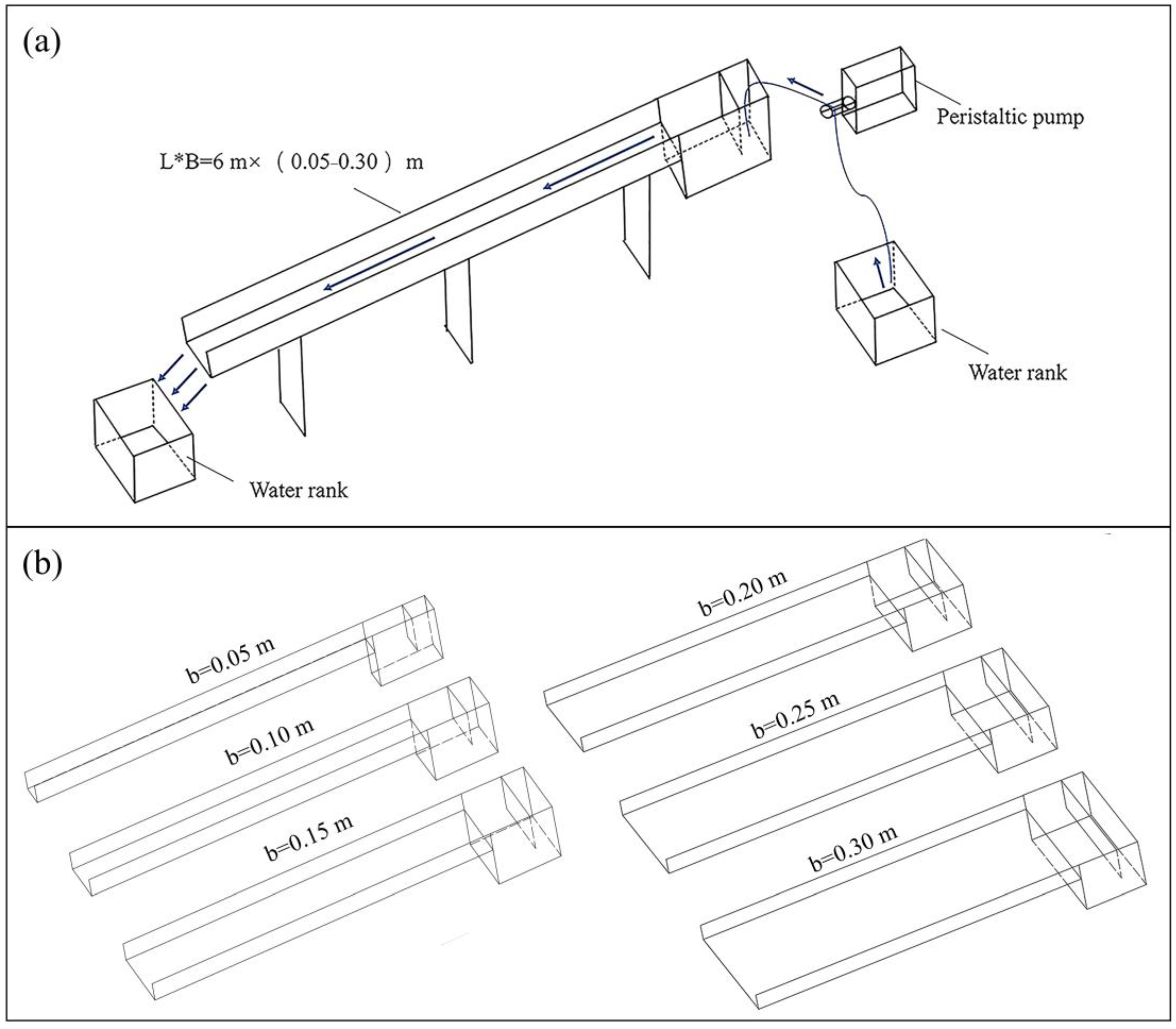
2.1. Experimental Setup

The experiment was carried out at the Science and Technology Research Center for Soil and Water Conservation Laboratory of Fujian Agriculture and Forestry University. The experimental setup mainly consisted of a hydraulic flume and a water supply system (Figure 1). Six different widths of flumes were designed. The flumes were made of galvanized steel sheets. The flume had the same length and height. The flumes were 6 m long, 0.05–0.30 m wide and 0.05 m high. The bed slope of the flume could be adjusted from 0° to 20°. Flow discharge was controlled by a peristaltic pump (model WT600-4F-C; Longer Pump Ltd., Baoding, Hebei Province, China). For each experiment, the slope gradients and flow discharges were adjusted to the designated values before the experiment. The test involved water flowing into a tank from an inlet pipe. A peristaltic pump was utilized to precisely regulate the discharge flow rate over narrow ranges during the test. Steady flow plates were installed in the flume to smooth the water flow. The hydrodynamic characteristics of overland flow on a slope were analyzed by measuring flow variables, such as discharge and velocity [3].

2.2. Experimental Design

The slope in this experiment was set according to the most common standard runoff plot slope, which was 15° [47]. There were six kinds of working conditions for the different widths of the flumes. The widths of the flume in this experiment were 0.05, 0.1, 0.15, 0.20, 0.25 and 0.30 m. The flow discharge per unit width (q) for each set of experiments was set up (0.33 × 10⁻⁴, 0.67 × 10⁻⁴, 1.00 × 10⁻⁴, 1.33 × 10⁻⁴, 1.67 × 10⁻⁴ m2 s−1). To facilitate narration and expression, the following text will adopt 0.02, 0.04, 0.06, 0.08 and 0.10 m2 min−1. The water temperature was measured using a thermometer with an accuracy of 0.1 °C. The specific experimental conditions are detailed in Table 2.
Flow velocities (surface velocity vs) were measured using KMnO4 within 2 m distances along the slope from the top test section to the bottom section [6,48,49]. The time interval for the tracer to move from the outset section to the end section was observed and measured using a digital stopwatch. From Figure 2, it can be observed that nine test sections were positioned at 0.0, 0.5, 1.0, 1.5, 2.0, 2.5, 3.0, 3.5 and 4.0 m along the experimental flume (the location 0.0 m is the point set at 10 cm from the flow inlet to further explore the effect of the width of the flume on the flow acceleration at the inlet of the flume.). To improve the accuracy of measurement, each test section is measured for water flow velocity at three measurement points, namely left, middle and right, with a distance of 1 cm between the left and right measurement points and the side wall [50,51]. The measurement points in the middle are located at the center of flume of various widths. The average flow velocity (v) is calculated by multiplying the surface flow velocity (vs) by a correction factor (α). The average flow velocity correction coefficient for laminar flow was generally 0.67, while the correction coefficients for transitional flow and turbulent flow were 0.7 and 0.8, respectively [48]. The overland flow was shallow, and it was difficult to measure its depth. Thus, the overland flow depth was calculated using flow velocities (Table 3).

2.3. Calculations of the Hydraulic Parameters

2.3.1. Flow Depth (h)

The depth of overland flow was calculated as follows [52]:
h = Q/vb
where h = the average water depth (m); Q = the discharge (L·min−1); v = the average water velocity (m·s−1) (the average water velocity refers to the average of the surface flow velocities at three points (left, middle, right) on the observed cross-section, after multiplying each velocity by a flow velocity correction factor); and b = the flume width (m).

2.3.2. Relative Average Deviation (RAD)

The relative average deviation (RAD) of velocity was calculated according to [53].
The RAD was used to judge the accuracy and representativeness of the arithmetic average.
The average deviation ( d ¯ ) is a statistical measure that computes the mean deviation from the average value of a given data collection and is calculated as follows:
d ¯ = i = 1 n x i x ¯ n
where x i = the average water velocity at each measurement point (m·s−1); x ¯ = the mean of the average water velocity at each measurement point (m·s−1); and n = sample size.
The RAD is defined as the proportion of the mean deviation and arithmetic mean. The RAD was calculated as follows:
R A D = d ¯ x ¯ × 100 %
where d ¯ is the average deviation, and x ¯ is the average value of velocity (m·s−1).

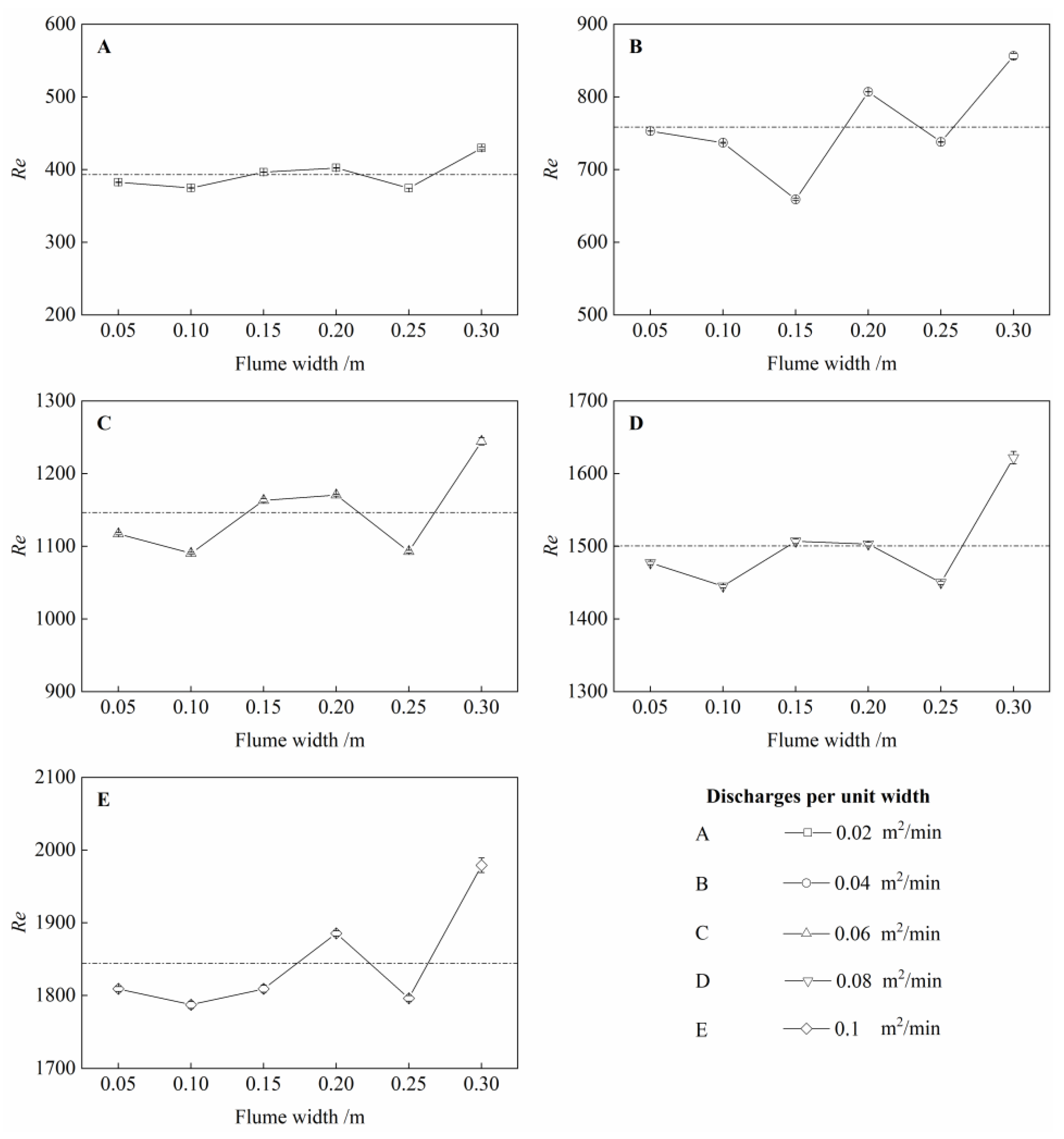
2.3.3. Reynolds Number (Re)

The Reynolds number helps to predict flow patterns in different fluid flow situations. The Reynolds number can be expressed as follows [54]:
Re = pvsR/η
where p = water density (kg/m3); vs = surface velocity (the average value of the surface flow velocity measured at each test point on all measurement cross-sections; R = the hydraulic radius (m): R = (hs b/b + 2*hs), hs = Q/vs; and η = the dynamic viscosity coefficient of overland flow (N·s/m2). The kinematic viscosity coefficient (μ = η/ρ) is very sensitive to varying temperatures, and μ can be calculated using Poiseuille’s equation as follows:
μ = 0.01775/(1 + 0.0337t + 0.000221t2)
where t = the water temperature.
The judgment criteria for Reynolds experiments were as follows: when Re < 500, the water flow is in the laminar flow regime; when 500 < Re < 5000, it falls into the transitional flow regime; and when Re > 5000, it is in the turbulent flow regime [19,55].

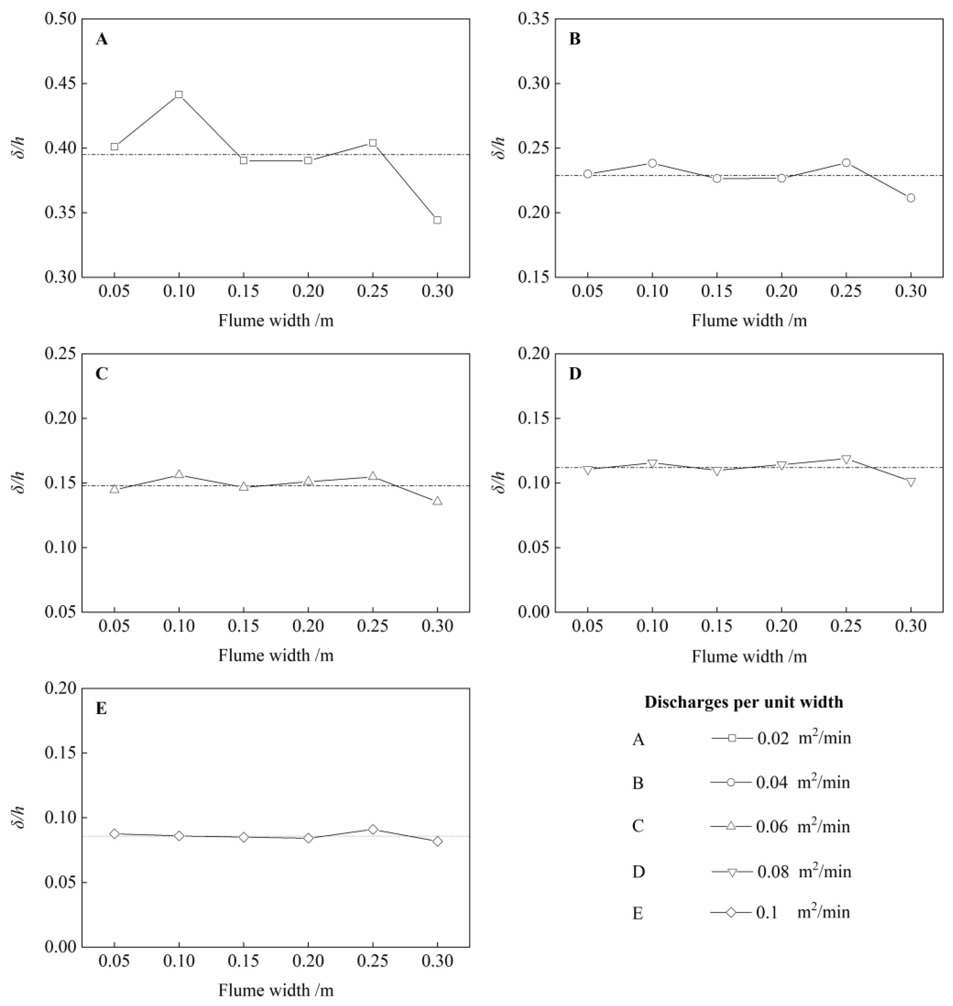
2.3.4. Flow Pattern Index (δ/h)

Zhang et al. [56] proposed a new method for defining the flow regime of overland flow by using a critical parameter δ/h, which is the ratio of the thickness of the viscous sublayer to the water depth. The viscous sublayer (δ) can be expressed as follows:
δ = 11.6v/u*
where u* = the shear velocity, which can be expressed as follows:
u* = (ghJ)0.5
where J = the hydraulic gradient approximated as sin θ, where θ is the gradient; in this study, θ = 15°, and g = acceleration due to gravity (9.80 m·s−2).
The flow pattern index (δ/h) can be expressed as follows:
ξ = δ/h = (11.6Fr)/(ReJ0.5)
The Froude number (Fr) is a dimensionless number defined as the ratio of the flow inertia to gravity. The Froude number of flow can be expressed as follows:
Fr = v/(gh)0.5

2.3.5. Specific Energy (Es)

When managing overland flow, it is convenient to reference the energy per unit weight from the channel bottom. The specific energy can be expressed as follows [57]:
E s = h + α Q 2 2 g A 2
where α = the kinetic energy correction coefficient, α = 1 [58,59,60]; and A = the cross-sectional area (cm2).
To explore the effect of the flume width on the specific energy change, the specific energy change can be expressed as follows [61]:
E S = h 2 h 1 + α Q 2 2 g A 2 2 α Q 2 2 g A 1 2
where h1 = the average water depth of the cross-section near the flume entrance (section at 0.0 m), h2 = the average water depth of the cross-section near the flume outlet (section at 4.0 m), A1 = the cross-sectional area near the flume entrance, and A2 = the cross-sectional area near the flume outlet.

3. Results

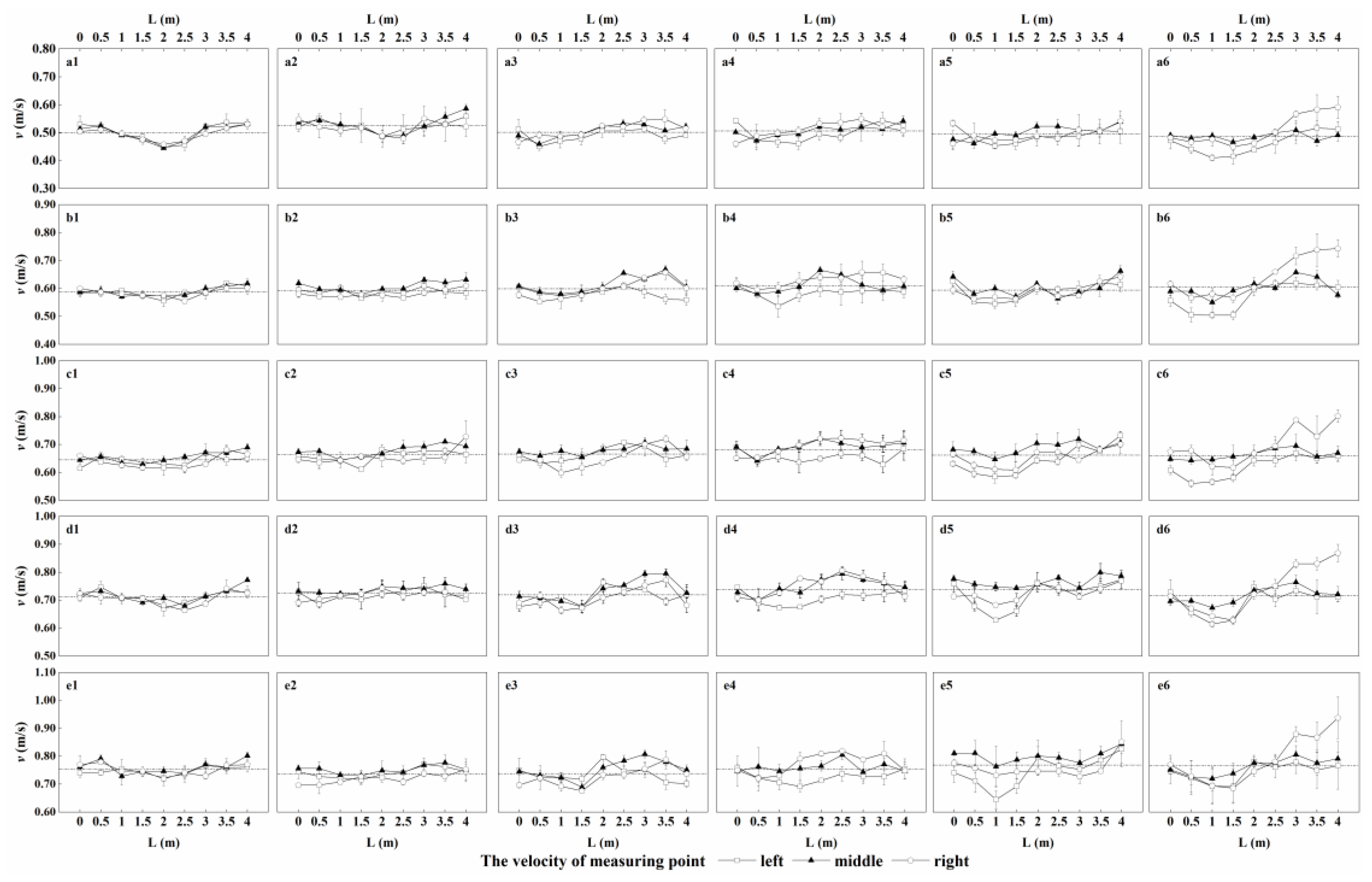
3.1. Flow Velocity Measurement under Different Widths

It is well known that the flow in the flume experiment is not unstable at first. At the beginning of the experiment, the water accelerates on the slope bed. The flow reaches a relatively stable state after a short distance. Figure 3 shows the variation in the flow velocities on the nine measurement sections in the different experiments. The flow velocity displays the tendency to decline at the beginning and rise late. At the same flow discharge per unit width, as the flume width increased, the downwards trend of flow velocities differed. The velocity decreased at the 0–2 m section when the flume width was 0.05 m. The fluctuation of velocity was not apparent with a width of 0.10 m. However, the flow velocities at the 0–1.5 m section decreased when the flume width ranged from 0.15 to 0.30 m.
As the flow discharge per unit width was increased, the difference in flow velocities at the three measurement points gradually increased. When the discharge per unit width was small, the three velocity curves in each group tended to coincide, which revealed that the difference in velocities at the three measurement points was small. As the discharge per unit width increased, the three velocity curves in each group tended to be discrete, and the velocity difference became large. As the flow flume width increased, the difference in velocity was similar to the condition of increasing discharge, but the flume width had more impact on velocity than discharge. In order to more clearly analyze the differences in flow velocity at different sections of the left, middle and right measuring points, a variance analysis was performed on the flow, width and flow velocity at each measuring point. The results are shown in Table 4. From the variance analysis, it can be seen that width, measuring point position and flow all have an extremely significant influence on flow velocity. From the results of the pairwise comparisons, when the width is 0.05–0.15 m, the flow velocities measured at different measuring points have relatively small significant differences. When the slot width is 0.20–0.30 m, the opposite is true. Under large flow conditions, the flow velocities measured at different measuring points differ more than those measured under small flow conditions.
Figure 4 shows the average flow velocity data measured at the left, middle and right measuring points at each section. For different widths, the difference between different widths at the 0–1.5 m sections show a trend of first decreasing and then increasing as the discharge increases. Under small discharge, the difference between different widths increases through the 2–3 m section and then gradually stabilizes. As the discharge increases, the difference between different widths increases to large values in the 2–3.5 m section, then it becomes smaller after 3.5 m.
To express the effect of flume width on velocity, the RAD of velocity was calculated (Figure 5). Under the different discharges, the values of RAD gradually increased as the flume width increased. The RAD of a narrow flume (the flume width was 0.05–0.1 m) was smaller than that of the others. When the flume width was 0.3 m, the highest RAD occurred. Through the variance analysis of the RAD under different widths at different flows, it can be seen that the RAD has extremely significant differences between different widths when the flow is 0.02–0.08 m2/min. However, there is no significant difference in the RAD under different widths when the flow is 0.10 m2/min. In addition, it can be seen from pairwise comparisons that the difference in the RAD of the 0.30 m slot width compared to other widths gradually decreases as the flow increases. When the flow is 0.02–0.04 m2/min, the RAD of the 0.30 m slot width has significant differences from other widths. When the flow reaches 0.10 m2/min, the 0.30 m slot width only has a significant difference with the 0.05 m slot width. Under all flow conditions, the RAD between widths of 0.10 to 0.25 m has no significant difference.

3.2. The Flow Pattern under Different Widths

Figure 6 indicates how the distribution of the Reynolds number varied with flume width and discharge change. Except for case (a), the Reynolds number of all cases varied from 650 to 2000. According to the judgment criteria of Reynolds experiments, the flow pattern of the water flow in this study belonged to the laminar and transitional flow range. The effect of the increasing flume width on the Reynolds number was not apparent for case (a). The Reynolds number showed a downwards trend when the flume width ranged from 0.05 to 0.10 m and from 0.20 to 0.25 m in all cases. Furthermore, the Reynolds number showed an upwards trend when the flume width ranged from 0.25 to 0.30 m. Table 1 shows that the common flume widths for laboratory simulations are 0.1, 0.2 and 0.3 m (these points are called particular points in our experiment). Table 5 shown the variation law of the Reynolds number of the flume width at specific points under different discharge conditions. The Reynolds number increased with increasing flume width under the different discharge conditions when the flume width was 0.10 m, 0.20 m and 0.30 m. Moreover, as the discharge increased, the effect of the flume width on the Reynolds number became more apparent.
However, while Re can demonstrate the alterations in flow patterns due to multiple factors such as roughness and slope, it has limitations in elucidating the phenomena of escalating resistance, sediment exchange and the instability of overland flow [3,62]. On the other hand, δ/h provides an intuitive representation of the movements of overland flow, the rolling waves indeed exist in this study in the experiment. Therefore, apart from employing the Reynolds number, the δ/h was also utilized to assess the flow pattern in this study in the course of this research. Zhang et al. [56] proposed that the critical value of δ/h can show the type of flow pattern. When δ/h ≥ 0.12, the flow regime exists in a laminar instability zone or rolling-wave flow zone. Otherwise, it exists in the turbulent flow zone. Figure 7 shows that the flume width affected δ/h. According to the judgment criteria of δ/h, when the discharge was 0.02–0.04 m2/min, roll waves would be generated in the water flow, and when the discharge was 0.08–0.10 m2/min, the flow regime of the water flow was turbulent flow. However, the water flow under different flume widths can be defined as a mixed-flow zone consisting of laminar instability and turbulent flow zones in case (c) [3]. The rolling-wave flow disappeared when the flume width was 0.30 m. However, the other widths of the flow patterns were still in the rolling-wave flow zone.

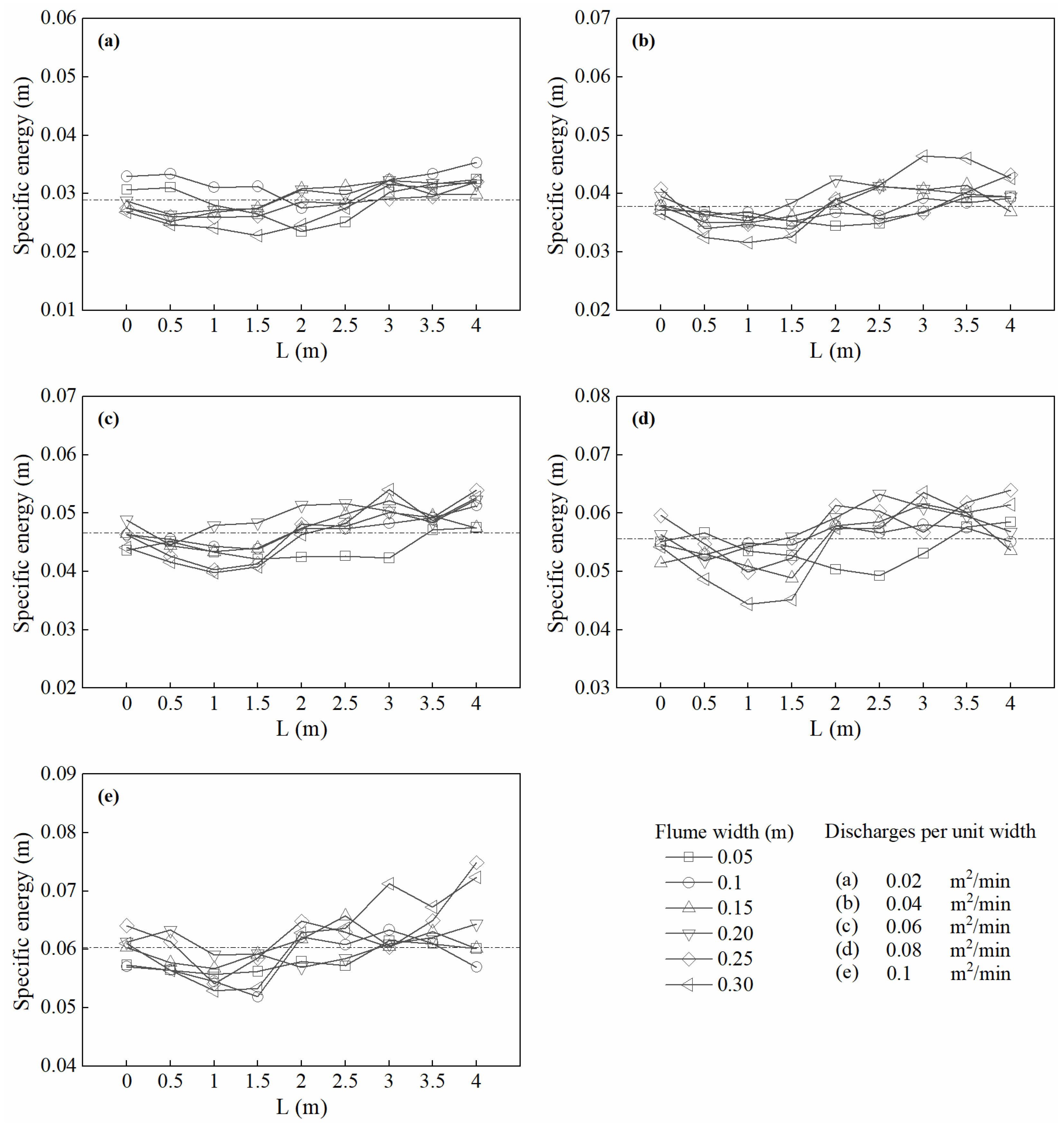
3.3. The Specific Energy under Different Widths

The data in Figure 8 show that the flume width affected the specific energy under different flow discharges. As the flow discharge per unit width increased, the difference in the specific energy for the flume widths gradually increased. As the discharge increased, a characteristic phenomenon was that the fluctuating range of the specific energy curve was not the same under different flume widths. The data can be divided into three sections according to the changing trend of the curve. In case (a), the discharge per unit width was small, and the difference in the specific energy on the different flume widths was also slight. When the discharge per unit width increased, the difference became larger in case (b) and case (c). The difference in the specific energy on the different flume widths reached the maximum in case (d) and case (e).
The variance was calculated by the specific energy at measurement points under different flume width conditions to express the fluctuating range of the specific energy curve under different flume width conditions. Figure 9 shows the cumulative percentage variance in the specific energy of different discharges. There were fewer fluctuations in the specific energy when the flume width ranged from 0.05 to 0.10 m under all discharge per unit width conditions except for 0.02 m2 min−1. However, there were violent fluctuations in the specific energy when the flume width ranged from 0.25 to 0.30 m. When the flume width was 0.20 m, the fluctuations in the specific energy were smaller than 0.25–0.3 m under all discharge per unit width conditions.
The data in Figure 10 show that the flume width affected the specific energy change (∆Es) under different flow discharges. The data can be divided into three sections according to the change trend of the curve. In case (a), the discharge per unit width was small, as were the fluctuations in ∆Es of the different flume widths. As the width increased, the effect of the flume width on ∆Es was not apparent for case (a). When the discharge per unit width increased, the difference became larger. The specific energy change of the different flume widths exhibited the same degree of fluctuation from case (b) to case (d). However, violent fluctuations in the specific energy of the different flume widths appeared in case (e). There were fluctuations in ∆Es when the flume width ranged from 0.05 to 0.15 m under all discharge per unit width conditions except for 0.02 m2 min−1. The ∆Es had an overall downwards trend with increasing width. In most cases, the specific energy change increased as the flume width increased when the flume width ranged from 0.15 to 0.30 m. Under the discharge per unit width condition, except for 0.02 m2 min−1, the fluctuations in ∆Es reached the minimum when the flume width was 0.15 m or 0.20 m.

4. Discussion

4.1. Flume Width and Velocity Measurement

In this work, the velocity of each flume width reached a relatively stable state at a long distance. This result is consistent with the experimental results obtained by Wang et al., Mujtaba and Yang et al. [63,64,65]. However, in our experiments, we find that velocity decelerated at the beginning of the experiment. The narrow flume had a specific restrictive effect on the acceleration of flow. This phenomenon may have been caused by the resistance of the narrow flume affecting the flow’s energy distribution. The flow acceleration was due to the mutual conversion between potential and kinetic energy. The sidewalls of the narrow flume generated more significant resistance and consumed power.
In our experiments, it was found that the width led to certain differences in the flow velocity measured at different measuring positions. The fundamental reason for this phenomenon is the result of the interaction between the width and the flow rate, as well as the interaction between the width and the measuring point position. The reason for the gradual increase in the differences between the measuring points when the width was 0.20–0.30 m may be due to the influence of the wall effect. When the water trough width is narrow, the distance between the measuring points is relatively close, and the difference between the wall area and the center area of the trough is relatively small. As the width of the water trough increases, the center area of the trough expands, while the area affected by the wall effect is still near the trough wall. In addition, the flow velocity change in the wall area of the tank is greater, while that in the center area is smaller [66]. Therefore, the difference in flow velocity measured at different flow velocity measuring points increases significantly. This is similar to the research results of Han et al. and Wang et al. [67,68]. The difference is that the research objects are different. The scholars above studied open channel flow, while the research object of this study is overland flow, so there are certain differences in the change in flow velocity with width.
From the changes in the average values, we can observe that within the range of measurement points from 1 m to 4 m along the flume, the water flow velocity exhibits an increasing trend across various widths. This result is consistent with the findings of Wang et al. [64], indicating that the flow velocities observed in this study conform to the fundamental principles of overland flow movement. In addition, our research also found that different widths have certain variation laws on the average value of each section. The differences in the width of the flume are mainly concentrated in the 2–3.5 m section. Within this range, the flow velocity of the high width gradually exceeds the flow velocity of the low width (0.30 m > 0.05 m). This result is the same as that obtained by Li [69]. This also indicates that the influence of width on flow velocity is not constant but rather exhibits variations that change with the length of the flume. At the inlet section, the flow is primarily influenced by spillage, resulting in acceleration. Different widths exhibit varying abilities to restrict water acceleration, and this capacity is significantly influenced by the flow rate. The reasons for the along-channel variations in the impact of different widths on flow velocity may be related to the occurrence and development of roll waves. The measurement range in this study is similar to the development and mature zones of rolling waves [49]. Wang et al. [64] proposed that rolling waves can cause significant fluctuations in flow velocity and water depth. However, the impact of flume width on rolling waves remains unexplored and should be further investigated in future studies.
The multipoint average algorithm has been widely used in overland flow experiments [2,4,70]. The RAD is a percentage of how much, on average, each measurement differs from the arithmetic average. The larger the value of RAD is, the more significant the difference between the values and the arithmetic average. In our study, RAD essentially represents the degree of influence of the sidewall effect on the flow velocity. As we described in the previous section, the sidewall effect is the most fundamental cause of the differences between measurement points at different locations. The greater these differences, the greater the value of RAD. Statistical analysis shows that this effect decreases gradually with increasing flow. This indicates that the sidewall effect has a greater impact on water flow measurement under low flow conditions. In addition, we note that the RAD values between 0.10 and 0.25 m are basically similar under different flows, and their RAD values are moderate, indicating that the impact of the sidewall effect they receive is relatively analogous. Therefore, when conducting flow velocity measurement experiments, flumes with widths between 0.10 and 0.25 m should be preferred in order to reduce the impact of sidewall effects on the flow velocity measurement results.

4.2. Flume Width and Roll-Wave Development

This study explored flow patterns at different widths based on Re and δ/h. Overland flows are divided into three categories by the Reynolds number: laminar flow, transition flow and turbulent flow. The results of this study indicate that, based on the Reynolds experiment as a criterion, the water flow in this study falls within the laminar and transitional regions. The results show that when using the traditional discriminant principles (Re), the flow patterns at different widths have no difference. However, there is no uniform standard for the classification of flow patterns in previous studies. Abrahams et al. [12] referred to the criterion of flow patterns (2000 < Re < 8000). Zhang et al. [24]. proposed that the criterion of Re is 580–6500. Notably, although Re can show how flow patterns vary with numerical factors, it is limited because it cannot explain the increasing-resistance phenomenon and instability phenomenon of overland flow [3].
In his research, Zhang [62] compared criteria for different flow patterns and introduced the viscous depth ratio as a criterion for determining the occurrence of roll waves in overland flow. Wang et al. [3] found that the critical parameter δ/h is better than the Reynolds number to study flow regimes. δ/h depicts the rolling waves of overland flow intuitively. The equation better reflects the ratio of three forces (viscous forces, inertial forces and gravity). When the discharge was small, the experimental flow could be defined as the rolling-wave flow. The flow would likely exist in the turbulent zone as the discharge increased. The rolling wave phenomenon weakened or disappeared, which is consistent with the results of Zhang et al. [56]. The results of this study reveal that, under specific flow conditions, the width influences the occurrence of roll waves. Possible reasons are as follows. When the discharge continued to increase, the experimental flows gradually approached the turbulent region. According to Figure 6 and Figure 9, this experiment demonstrated that the flume width of 0.3 m had the highest degree of mixing (the Re and fluctuations in the specific energy were more extensive than other widths). The large discharge affects the resistance laws, transforming the proportional relation between resistance and discharges into a square relation [49]. The body of water tends to balance, and the rolling wave phenomenon disappears. These inherent mechanisms are consistent with the experimental results obtained by Meng et al. [71].

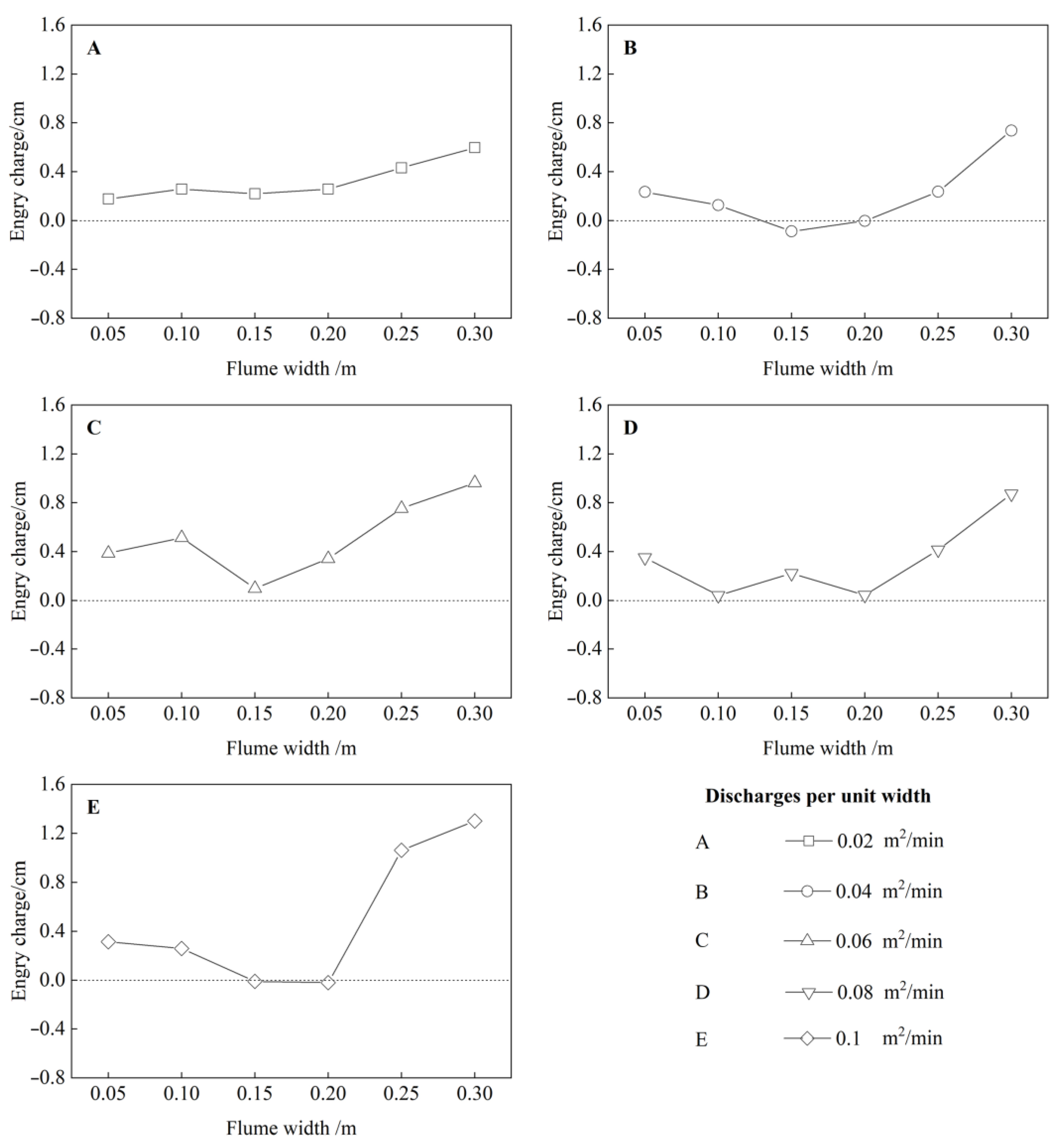
4.3. The Relationship between Width and ∆Es

The energy variation of a narrow flume was more minor than that of a wide flume. The violent fluctuations in the specific energy indicated that the force condition of the fluid element was complicated along with the downslope distance in the flow direction. According to the first law of thermodynamics, the rate of change in the energy inside the fluid element is composed of the net flux of heat and the work done on the element by the body forces and surface forces [72]. This study showed no apparent change in the water temperature. The net flux of heat into the element was ignored. Thus, when the flume becomes wide, it could increase the effect of the body and surface forces on flow. The wide-to-depth ratio conditions for various widths in this experiment are shown in the Table 6. Many principles of calculation in overland flow are derived from open channel hydraulics. Currently, there is a knowledge gap in the research on how different widths affect the energy distribution in overland flow. Indeed, in the field of open channel hydraulics, there have been numerous studies exploring the relationship between sidewall effects and changes in energy as well as shear force distribution. Therefore, this section attempts to explore the influence of width on energy and shear stress in open channel flow, in order to further elucidate the impact of width on overland flow.
The relationship between changes in energy in open channel flow and the sidewall effects is as follows: Chien [73] proposed the flow energy conversion process. Most of the water flow energy comes from potential energy. The flow energy is transferred through the viscous effect. The direction of energy transfer is from the free surface to the bottom of the flume and from the flume’s central area to the flume’s sidewall. Bakhmeteff and Allan [74] inferred that the flow energy is transferred to the near-wall region due to the shear force. In the near-wall flow region, the energy is transformed into kinetic energy and partially dissipated as heat energy during the transformation. The cross-sectional shape primarily governs the boundary shear stress distribution [75,76]. The boundary shear stress of flows can be separated into bed shear stress and sidewall shear stress [77]. The distribution of the boundary shear stress at several width–depth ratios has been explored in several studies. Knight et al. [78] indicated a reduction in the mean wall shear stress with increasing b/h. In other words, the sidewall effect decreases with increasing b/h. The proportions of any water body’s energy transmitted to the sidewall and bed are different [79]. The fluid motion satisfies the minimum energy dissipation rate principle [80]. The flow energy will approach the near-wall region area with the shortest distance to achieve the minimum energy dissipation.
Due to the shallower water depth in overland flow, the wide-to-depth ratio in overland flow is significantly larger compared to open channels. Therefore, the energy transfer discussed above is more readily achievable in overland flow. The b/h increased rapidly with increasing width. The sidewall effect was smaller than the bed-surface effect when the flume width ranged from 0.20 to 0.30 m. The flow energy was mainly transferred to the bottom of the flume. This is also the reason why the change in energy ∆Es in a wide flume tends to increase.

5. Conclusions

The effect of the flume width on the hydraulic characteristics of overland flow has often been ignored in previous studies. This study systematically depicted the experimental phenomenon and investigated the velocity measurement, flow pattern and flow energy under different flume widths. The results of this study are described as follows:
With the increase in flume width, the flow velocity in the wider flume gradually becomes greater than that in the narrower flume Under the influence of the sidewall effect, increasing the channel width results in an increase in the differences in flow measurements at different measurement points.
The width has an impact on the flow patterns of water, and the magnitude of width affects the generation and evolution of roll waves. Using δ/h as a parameter proved more effective than Re in characterizing flow regimes across various flume widths, as it accurately depicted flow regimes in both the rolling-wave and turbulent flow regions.
Width affects the distribution of energy within the flume. Wider flumes led to energy fluctuations and elevated specific energy levels, with flumes of higher wide-to-depth ratios having energy distribution closer to the channel bottom rather than the channel walls.
In practical applications, especially when selecting a flume for overland flow experiments, it is advisable to evenly distribute the measurement points along the cross-section, particularly when using a wide flume for testing. This contributes to comprehensive measurement of water flow velocity.
These integrated results emphasize that the effect of the flume width on hydraulic characteristics cannot be ignored and can contribute to the theoretical foundation for studying the relationship between the flume width and the hydraulic characteristics of overland flow in order to further understand the hydraulic characteristics of overland flow and provide theoretical references for optimizing experimental design.

Author Contributions

Conceptualization, Y.T. and J.L.; data curation, Y.T., Y.X. and M.Y.; methodology, Y.T. and J.L.; supervision, J.L.; visualization, Y.T., Y.X. and M.Y.; writing—original draft preparation, Y.T.; writing—review and editing, Y.T., F.J., Y.Z., Y.H. and J.L. All authors have read and agreed to the published version of the manuscript.

Funding

This research was supported financially by the Disciplinary Innovation Team Support Program of Forestry (118/72202200205), the National Natural Science Foundation of China (41977071) and Demonstration of Rapid Dam Construction and Sediment Control Technology at the Mouth of Active Benggang (KKY22002XA).

Data Availability Statement

The data presented in this study are available within the article.

Conflicts of Interest

The authors declare no conflict of interest.

References

  1. Giménez, R.; Govers, G. Flow Detachment by Concentrated Flow on Smooth and Irregular Beds. Soil Sci. Soc. Am. J. 2002, 66, 1475–1483. [Google Scholar] [CrossRef]
  2. Liu, Y.M.; Zhang, G.H.; Li, L.J.; Han, Y.F. Quantitative effects of hydrodynamic parameters on soil detachment capacity of overland flow. Trans. Chin. Soc. Agric. Eng. 2009, 25, 96–99. [Google Scholar]
  3. Wang, J.W.; Lv, X.R.; Zhang, K.D.; Li, P.; Meng, H. Unsteady-State Hydraulic Characteristics of Overland Flow. J. Hydrol. Eng. 2019, 24, 04019046. [Google Scholar] [CrossRef]
  4. Zhan, Z.Z.; Jiang, F.S.; Chen, P.S.; Gao, P.Y.; Lin, J.S.; Ge, H.L.; Wang, M.K.; Huang, Y.H. Effect of gravel content on the sediment transport capacity of overland flow. Catena 2020, 188, 104447. [Google Scholar] [CrossRef]
  5. Zhang, G.H.; Liu, B.Y.; Liu, G.B.; He, X.W.; Nearing, M.A. Detachment of undisturbed soil by shallow flow. Soil Sci. Soc. Am. J. 2003, 67, 713–719. [Google Scholar] [CrossRef]
  6. Zhang, G.H.; Luo, R.T.; Cao, Y.; Shen, R.C.; Zhang, X.C. Correction factor to dye-measured flow velocity under varying water and sediment discharges. J. Hydrol. 2010, 389, 205–213. [Google Scholar] [CrossRef]
  7. Zhao, C.H.; Gao, J.E.; Huang, Y.F.; Wang, G.Q.; Zhang, M.J. Effects of Vegetation Stems on Hydraulics of Overland Flow under Varying Water Discharges. J. Irrig. Drain. Eng. 2016, 27, 748–757. [Google Scholar] [CrossRef]
  8. Chen, H.; Zhang, X.P.; Abla, M.; Lu, D.; Yan, R.; Ren, Q.F.; Ren, Z.Y.; Yang, Y.H.; Zhao, W.H.; Lin, P.F.; et al. Effects of vegetation and rainfall types on surface runoff and soil erosion on steep slopes on the Loess Plateau, China. Catena 2018, 170, 141–149. [Google Scholar] [CrossRef]
  9. Cai, W.L.; Huang, H.; Chen, P.N.; Huang, X.L.; Gaurav, S.; Pan, Z.; Lin, P. Effects of biochar from invasive weed on soil erosion under varying compaction and slope conditions: Comprehensive study using flume experiments. Biomass Convers. Biorefin. 2020. [Google Scholar] [CrossRef]
  10. Cheng, N.S.; Hui, C.L.; Wang, X.K.; Tan, S.K. Laboratory Study of Porosity Effect on Drag Induced by Circular Vegetative Patch. J. Eng. Mech. 2019, 145, 04019046. [Google Scholar] [CrossRef]
  11. Wang, J. Shallow Flow Hydraulics on a Hillslope and Evolution of Roll Waves under Artificial Rainfall Conditions. Master’s Thesis, Northwest A&F University, Xianyang, China, 2016. [Google Scholar]
  12. Abrahams, A.D.; Li, G. Effect of saltating sediment on flow resistance and bed roughness in overland flow. Earth Surf. Process. Landf. 1998, 23, 953–960. [Google Scholar] [CrossRef]
  13. Abrahams, A.D.; Parsons, A.J.; Wainwright, J. Resistance to overland flow on semiarid grassland and shrubland hillslopes, Walnut Gulch, Southern Arizona. J. Hydrol. 1994, 156, 431–446. [Google Scholar] [CrossRef]
  14. Xia, W.S.; Lei, T.W.; Zhang, Q.W.; Zhao, J. Electrolyte Pulse Migration Model in Shallow Surface Flow on Slopes. J. Hydraul. Eng. 2003, 11, 90–95. [Google Scholar]
  15. Emmett, W.W. The Hydraulics of Overland Flow on Hillslopes; US Government Printing Office: Washington, DC, USA, 1970; Volume 662.
  16. Li, X.; Huang, Y.; Lin, J. Effects of different width of scouring flumes on runoff and sediment yield of colluvial deposits of collapsing hill. Trans. Chin. Soc. Agric. Eng. 2016, 32, 136–141. [Google Scholar]
  17. Wang, W.; Li, X.Y.; Zhang, J.; Liu, Q.; Lei, T.W. Experimental Study of Runoff Velocity Measurement System Based on Conductivity Sensor. Trans. Chin. Soc. Agric. Eng. 2007, 2, 1–5. [Google Scholar]
  18. Bai, K.Q.; Zhu, Y.; Tian, Y.; Ye, D.P. Construction and Experimental Study of a Shallow Water Flow Velocity Measurement System Based on Photoelectric Sensing Technology. J. Soil Water Conserv. 2021, 35, 34–40. [Google Scholar] [CrossRef]
  19. Yang, P.P.; Zhang, H.L.; Wang, Y.Q.; Li, R. Particle Image Velocimetry-based Hydrodynamic Characteristics of Surface Flow on Slopes. Trans. Chin. Soc. Agric. Eng. 2020, 36, 115–124. [Google Scholar]
  20. Wu, S.F.; Wu, P.T.; Yuan, L.F. Experimental Study on Hydraulic Characteristics of Surface Runoff Control and Shallow Water Flow on Slopes. Trans. Chin. Soc. Agric. Eng. 2010, 26, 14–19. [Google Scholar]
  21. Zhu, Y.; Luo, Q.; Tian, Y. Development of the depth measurement system for shallow flow on slopes using an edge-detection algorithm. Trans. Chin. Soc. Agric. Eng. 2022, 38, 157–165. [Google Scholar]
  22. Horton, R.E. Erosional development of streams and their drainage basins; hydrophysical approach to quantitative morphology. Geol. Soc. Am. Bull. 1945, 56, 275–370. [Google Scholar] [CrossRef]
  23. Shang, J.D.; Jiang, X.J. On the Fundamental Dynamic Characteristics of Shallow Water Flow on Erosive Slopes in Initial Ecological Conditions. J. Soil Water Conserv. 1995, 09, 29–35. [Google Scholar]
  24. Zhang, K.D.; Wang, G.Q.; Sun, X.M.; Yang, F.; Lv, H.X. Experimental Study on Hydraulic Characteristics of Shallow Surface Flow on Slopes. Trans. Chin. Soc. Agric. Eng. 2014, 30, 182–189. [Google Scholar]
  25. Grayson, R.B.; Moore, I.D. Effect of land-surface configuration on catchment hydrology. In Overland-Flow: Hydraulics and Erosion Mechanics; CRC Press: Boca Raton, FL, USA, 1992; p. 393407. [Google Scholar] [CrossRef]
  26. Scoging, H.; Parsons, A.J.; Abrahams, A.D. Application of a dynamic overland-flow hydraulic model to a semi-arid hillslope, Walnut Gulch, Arizona. In Overland Flow: Hydraulics and Erosion Mechanics; CRC Press: Boca Raton, FL, USA, 1992; pp. 105–145. [Google Scholar] [CrossRef]
  27. Abrahams, A.D.; Parsons, A.J.; Hirsch, P.J. Field and laboratory studies of resistance to interrill overland flow on semi-arid hillslopes, southern Arizona. In Overland Flow: Hydraulics and Erosion Mechanics; CRC Press: Boca Raton, FL, USA, 1992; pp. 1–23. [Google Scholar] [CrossRef]
  28. Hu, S.X.; Abrahams, A.D. Resistance to overland flow due to bed-load transport on plane mobile beds. Earth Surf. Process. Landf. 2004, 29, 1691–1701. [Google Scholar] [CrossRef]
  29. Noarayanan, L.; Murali, K.; Sundar, V. Manning’s ‘n’ co-efficient for flexible emergent vegetation in tandem configuration. J. Hydro-Environ. Res. 2012, 6, 51–62. [Google Scholar] [CrossRef]
  30. Ma, L.; Pan, C.Z.; Liu, J.J. Overland flow resistance and its components for slope surfaces covered with gravel and grass. Int. Soil Water Conserv. Res. 2022, 10, 273–283. [Google Scholar] [CrossRef]
  31. Darboux, F.; Davy, P.; Gascuel-Odoux, C.; Huang, C. Evolution of soil surface roughness and flowpath connectivity in overland flow experiments. Catena 2002, 46, 125–139. [Google Scholar] [CrossRef]
  32. Hu, S.X.; Abrahams, A.D. The effect of bed mobility on resistance to overland flow. Earth Surf. Process. Landf. 2005, 30, 1461–1470. [Google Scholar] [CrossRef]
  33. Bond, S.; Kirkby, M.J.; Johnston, J.; Crowle, A.; Holden, J. Seasonal vegetation and management influence overland flow velocity and roughness in upland grasslands. Hydrol. Process. 2020, 34, 3777–3791. [Google Scholar] [CrossRef]
  34. Fu, S.; Mu, H.; Liu, B.; Yu, X.; Liu, Y. Effect of plant basal cover on velocity of shallow overland flow. J. Hydrol. 2019, 577, 123947. [Google Scholar] [CrossRef]
  35. Zhao, L.Y.; Zhang, K.D.; Wu, S.F.; Feng, D.Q.; Shang, H.X.; Wang, J.W. Comparative study on different sediment transport capacity based on dimensionless flow intensity index. J. Soils Sediments 2020, 20, 2289–2305. [Google Scholar] [CrossRef]
  36. Shen, H.W.; Li, R.-M. Rainfall Effect on Sheet Flow over Smooth Surface. J. Hydraul. Div. 1973, 99, 771–792. [Google Scholar] [CrossRef]
  37. Wang, J.W.; Zhang, K.D.; Gong, J.G.; Yang, F.; Ma, X. Influence of rainfall and slope gradient on resistance law of overland flow. J. Irrig. Drain. 2016, 35, 43–49. [Google Scholar] [CrossRef]
  38. Yang, P.; Wang, Y.Q.; Zhang, H.L.; Wang, Y.J. Characteristics of overland flow resistance under interaction of rainfall intensity and unit discharge and surface roughness. Trans. Chin. Soc. Agric. Eng. 2018, 34, 145–151. [Google Scholar]
  39. Jomaa, S.; Barry, D.A.; Brovelli, A.; Sander, G.C.; Parlange, J.Y.; Heng, B.C.P.; Tromp-van Meerveld, H.J. Effect of raindrop splash and transversal width on soil erosion: Laboratory flume experiments and analysis with the Hairsine–Rose model. J. Hydrol. 2010, 395, 117–132. [Google Scholar] [CrossRef]
  40. Williams, G.P. Flume Width and Water Depth Effects in Sediment-Transport Experiments; US Government Printing Office: Washington, DC, USA, 1970.
  41. Ciampalini, R.; Torri, D. Detachment of soil particles by shallow flow: Sampling methodology and observations. Catena 1998, 32, 37–53. [Google Scholar] [CrossRef]
  42. Ma, R.M.; Cai, C.F.; Wang, J.G.; Wang, T.W.; Li, Z.X.; Xiao, T.Q.; Peng, G.Y. Partial least squares regression for linking aggregate pore characteristics to the detachment of undisturbed soil by simulating concentrated flow in Ultisols (subtropical China). J. Hydrol. 2015, 524, 44–52. [Google Scholar] [CrossRef]
  43. Nearing, M.A.; Bradford, J.M.; Parker, S.C. Soil Detachment by Shallow Flow at Low Slopes. Soil Sci. Soc. Am. J. 1991, 55, 339–344. [Google Scholar] [CrossRef]
  44. Poesen, J.; De Luna, E.; Franca, A.; Nachtergaele, J.; Govers, G. Concentrated flow erosion rates as affected by rock fragment cover and initial soil moisture content. Catena 1999, 36, 315–329. [Google Scholar] [CrossRef]
  45. Sun, B.Y.; Xiao, J.B.; Li, Z.B.; Ma, B.; Zhang, L.T.; Huang, Y.L.; Bai, L.F. An analysis of soil detachment capacity under freeze-thaw conditions using the Taguchi method. Catena 2018, 162, 100–107. [Google Scholar] [CrossRef]
  46. Wang, D.; Wang, Z.; Shen, N.; Chen, H. Modeling soil detachment capacity by rill flow using hydraulic parameters. J. Hydrol. 2016, 535, 473–479. [Google Scholar] [CrossRef]
  47. Zhang, K.L.; Liu, B.Y.; Cai, Y.M. The standard of unit plot in soil loss prediction of China. Geogr. Res. 2000, 19, 297–302. [Google Scholar]
  48. Abrahams, A.D.; Parsons, A.J.; Luk, S.-H. Field measurement of the velocity of overland flow using dye tracing. Earth Surf. Process. Landf. 1986, 11, 653–657. [Google Scholar] [CrossRef]
  49. Wang, J.W.; Zhang, K.D.; Li, P.; Meng, Y.; Zhao, L.Y. Hydrodynamic characteristics and evolution law of roll waves in overland flow. Catena 2021, 198, 105068. [Google Scholar] [CrossRef]
  50. Jing, X.F. Study on Hydraulic Properties of Shallow Flow on Slope Surface. Master’s Thesis, Northwest A&F University, Xianyang, China, 2007. [Google Scholar]
  51. Shi, M.X. Influence of Surface Roughness on Hydraulic Characteristics of Overland Flow. Master’s Thesis, Northwest A&F University, Xianyang, China, 2015. [Google Scholar]
  52. Jiang, F.S.; He, K.W.; Huang, M.Y.; Zhang, L.T.; Lin, G.G.; Zhan, Z.Z.; Li, H.; Lin, J.S.; Ge, H.L.; Huang, Y.H. Impacts of near soil surface factors on soil detachment process in benggang alluvial fans. J. Hydrol. 2020, 590, 125274. [Google Scholar] [CrossRef]
  53. Hu, Q.; Chen, J. Analytical Chemistry, 2nd ed.; Huazhong University of Science and Technology Press Co., Ltd.: Wuhan, China, 2020; p. 242. [Google Scholar]
  54. Reynolds, O. XXIX. An Experimental Investigation of the Circumstances Which Determine Whether the Motion of Water Shall be Direct or Sinuous, and of the Law of Resistance in Parallel Channels; The Royal Society London: London, UK, 1997; pp. 935–982. [Google Scholar]
  55. Zhang, K.D.; Wang, G.Q.; Sun, X.M.; Wang, J.J. Hydraulic characteristic of overland flow under different vegetation coverage. Adv. Water Sci. 2014, 25, 825–834. [Google Scholar] [CrossRef]
  56. Zhang, K.D.; Wang, G.Q.; Lv, H.X.; Wang, Z.L. Discussion on flow pattern determination method of shallow flow on the slope surface. J. Exp. Fluid Mech. 2011, 25, 67–73. [Google Scholar]
  57. Bakhmeteff, B. O Neravnomernom Dwijenii Jidkosti v Otkrytom Rusle; KUBUCH: Saint Petersburg, Russia, 1912. [Google Scholar]
  58. Liu, J.E.; Wang, Z.L.; Gao, S.J.; Zhang, K.D. Experimental study on hydro-dynamic mechanism of sheet erosion processes on loess hillslope. Trans. Chin. Soc. Agric. Eng. 2012, 28, 144–149. [Google Scholar]
  59. Zhang, Q.; Zheng, S.Q.; Tian, F.X.; Ma, Y.C. Runoff and sediment yield characteristics of earth road under artificial rainfalland simulated overland flow tests conditions in Loess Plateau. Trans. Chin. Soc. Agric. Eng. 2010, 26, 83–87. [Google Scholar]
  60. Zhang, L.T.; Gao, Z.L.; Tian, H.W. Hydrodynamic process of soil erosion in steep slope of engineering accumulation. Trans. Chin. Soc. Agric. Eng. 2013, 29, 94–102. [Google Scholar]
  61. Belanger, J.B. Essai sur la Solution Numerique de Quelques Problemes Relatifs au Mouvement Permanent des Eaux Courantes; Chez Carilian-Goeury, Libraire: Paris, France, 1828. [Google Scholar]
  62. Zhang, K.D. Research on Hydrodynamic Characteristics of Slope Surface Flow and Sediment Transport Mechanisms; Northwest A&F University: Xianyang, China, 2011. [Google Scholar]
  63. Mujtaba, B.; de Lima, J.L.M.P. Laboratory testing of a new thermal tracer for infrared-based PTV technique for shallow overland flows. Catena 2018, 169, 69–79. [Google Scholar] [CrossRef]
  64. Wang, X.K.; Yan, X.F.; Zhou, S.F.; Huang, E.; Liu, X.N. Longitudinal variations of hydraulic characteristics of overland flow with different roughness. J. Hydrodyn. 2014, 26, 66–74. [Google Scholar] [CrossRef]
  65. Yang, D.M.; Gao, P.L.; Zhao, Y.D.; Zhang, Y.H.; Liu, X.Y.; Zhang, Q.W. Modeling sediment concentration of rill flow. J. Hydrol. 2018, 561, 286–294. [Google Scholar] [CrossRef]
  66. Yan, J.; Wang, E.P.; Sun, D.P.; Dong, Z.H. Experimental Study on Velocity Distribution Characteristics in Rectangular Cross-Section Open Channel. J. Wuhan Univ. (Eng. Ed.) 2005, 38, 59–64. [Google Scholar]
  67. Han, J.X.; Huang, F.G.; Xia, P.L.; Wu, Y.L.; Chen, W.W. Parabolic Law for Lateral Distribution of Flow Velocity in Open Channels and Its Applications. People’s Yellow River 2013, 35, 83–85. [Google Scholar]
  68. Wang, E.P.; Jin, H.; Wang, W.J.; Zhang, Y.Y.; Cao, B. Rectangular Open Channel Velocity Distribution Law and Automated Flow Measurement Methods. People’s Yellow River 2008, 30, 31–32. [Google Scholar]
  69. Li, X.Z. The Influence of Scour Trenches with Different Widths on the Erosion of Colluvial Deposits in Debris Flow Gullies. Master’s Thesis, Fujian Agriculture and Forestry University, Fuzhou, China, 2016. [Google Scholar]
  70. Zhang, G.H. Study on hydraulic properties of shallow flow. Adv. Water Sci. 2002, 13, 159–165. [Google Scholar]
  71. Meng, H.; Zhang, K.D.; Wang, J.W. Influence factors of hydraulic parameters of roll waves in overland flow. Adv. Water Sci. 2020, 31, 102–111. [Google Scholar] [CrossRef]
  72. Anderson, J.D.; Wendt, J. Computational Fluid Dynamics; McGraw-Hill: New York, NY, USA, 1995. [Google Scholar]
  73. Chien, N.; Wan, Z. Mechanics of Sediment Transport; American Society of Civil Engineers: New York, NY, USA, 1999; p. 1999. [Google Scholar]
  74. Bakhmeteff, B.A.; Allan, W. The mechanism of energy loss in fluid friction. Trans. Am. Soc. Civ. Eng. 1946, 111, 1043–1080. [Google Scholar] [CrossRef]
  75. Ghosh, N.S.; Roy, N. Boundary shear distribution in open channel flow. J. Hydraul. Div. 1970, 96, 967–994. [Google Scholar] [CrossRef]
  76. Knight, D.W.; Hamed, M.E. Boundary Shear in Symmetrical Compound Channels. J. Hydraul. Eng. 1984, 110, 1412–1430. [Google Scholar] [CrossRef]
  77. Einstein, H.A. Formulas for the Transportation of Bed Load. Trans. Am. Soc. Civ. Eng. 1942, 107, 561–577. [Google Scholar] [CrossRef]
  78. Knight, D.W.; Macdonald, J.A. Open Channel Flow with Varying Bed Roughness. J. Hydraul. Div. 1979, 105, 1167–1183. [Google Scholar] [CrossRef]
  79. Shen, H.B.; Zhang, X.F.; Qiao, W. Partition curve of hydraulic radius and average sidewall and bed shear stresses in open-channel flows. J. Hydrol. Eng. 2011, 30, 44–48. [Google Scholar]
  80. Xu, G.; Yang, C.T.; Zhao, L. Minimum Energy Dissipation Rate Theory and Its Applications for Water Resources Engineering. Adv. Water Resour. Eng. 2015, 14, 183–245. [Google Scholar] [CrossRef]
Figure 1. The experimental equipment of overland flow: (a) experimental setup used to measure velocity of overland flow; (b) experimental setup of different flume widths.
Water 15 03416 g001
Figure 2. The water velocity measurement location.
Water 15 03416 g002
Figure 3. The flow velocity for each flume width under different discharges per unit width. The letters (ae) in different figures represent various discharges per unit width from 0.02 to 0.1 m2/min with increments of 0.02 m2/min. The numbers 1–6 represent the tank width from 0.05 to 0.30 m with a step of 0.05 m. The velocities at measuring points are shown as squares, triangles and rhombuses. The dotted line represents a mean value within the group. Left y-axis shows the velocity of flow; x-axis shows nine test sections along the flume.
Water 15 03416 g003
Figure 4. The average flow velocity at the measurement section for each flume width under different discharges per unit width. The letters (AE) in different figures represent various discharges per unit width from 0.02 to 0.1 m2/min with increments of 0.02 m2/min. Each line segment in the figure represents a different width. Left y-axis shows the velocity of flow; x-axis shows nine test sections along the flume.
Water 15 03416 g004
Figure 5. Variation in relative mean deviation of velocity with different flume widths. The letters (AE) in different figures represent various discharges per unit width from 0.02 to 0.1 m2/min with increments of 0.02 m2/min. In the figure, the letters a–c represents the results of pairwise comparisons, and groups marked with the same letter indicate that they do not have significant differences.
Water 15 03416 g005
Figure 6. The Reynolds number varied with flume width. The dotted line represents a mean value within the group.
Water 15 03416 g006
Figure 7. Variation in flow pattern indices depending on the flume width. The dotted line represents a mean value within the group. Left y-axis shows the ratio of the thickness of the viscous sublayer to the water depth; x-axis shows different flume widths.
Water 15 03416 g007
Figure 8. The specific energy distributed under different flume widths. The letters (ae) in different figures represent various discharges per unit width from 0.02 to 0.1 m2/min with increments of 0.02 m2/min. The dotted line represents a mean value within the group. The solid lines show the specific energy of different flume widths. Left y-axis shows the specific energy; x-axis shows nine test sections located along the flume.
Water 15 03416 g008
Figure 9. The percent stacked bar chart for fluctuations in specific energy under various flume widths. This paper calculated the variance in specific energy of different flume widths under the same flow condition (Figure 8). The percent stacked bar chart was used to display variance data. The boxes of different colors in the same column represent the percentage of the variance for different flume widths. Left y-axis shows percentage of the variance in the specific energy; x-axis shows various discharges per unit width.
Water 15 03416 g009
Figure 10. The effect of flume width on specific energy change. The dotted line represents the value of zero. Left y-axis shows specific energy change; x-axis shows different flume widths.
Water 15 03416 g010
Table 1. Different designs of the flume width in previous studies.
ReferencesMaterialFlume Length (m)Flume Width (m)
Nearing et al., 1991 [43]/9.001.00
Ciampalini and Torri, 1998 [41]Plexiglass1.500.20
Poesen et al., 1999 [44]Plexiglass2.000.098
Govers, 2002 [1]Mixed4.300.40
Zhang et al., 2003 [5]/4.000.35
Ma et al., 2015 [42]Zincified sheet iron plate3.800.20
Wang et al., 2016 [46]/4.000.10
Sun et al., 2018 [45]Plexiglass1.000.04
Zhan et al., 2020 [4]Zincified sheet iron plate4.000.12
Table 2. The experimental conditions.
Slope (°)Flume Width (m)Discharge
per Unit Width
(×10−4 m2 s−1)
Water
Temperature
(°C)
Dynamic
Viscosity
(×10−4 N·s/m2)
150.05–0.300.33, 0.67, 1.00, 1.33, 1.67 25.1–32.57.62–8.8
Table 3. The overland flow depth (mm).
Discharge
per Unit Width
(×10−4 m2 s−1)
Flume Width (m)
0.050.10.150.20.250.3
0.330.449 0.427 0.446 0.442 0.453 0.463
0.670.795 0.788 0.781 0.768 0.787 0.779
1.001.091 1.054 1.053 1.029 1.062 1.067
1.331.312 1.291 1.302 1.271 1.269 1.311
1.671.550 1.583 1.584 1.550 1.524 1.534
Table 4. Pairwise comparisons of flow velocity at measuring points.
Flume Width (m)Discharges
per Unit Width
(m2/min)
Flow Velocity at
Measuring Points
LMR
0.050.02
0.04
0.06
0.08
0.1
0.10.02
0.04
0.06
0.08
0.1aabb
0.150.02
0.04aabb
0.06
0.08
0.1
0.20.02
0.04aab
0.06aab
0.08aab
0.1aab
0.250.02
0.04
0.06abb
0.08abb
0.1abb
0.30.02aabb
0.04abc
0.06abc
0.08aabc
0.1aabb
Note(s): The letters a–c represents the results of pairwise comparisons, and groups marked with the same letter indicate that they do not have significant differences.
Table 5. Variation in Reynolds number with flume width at specific point.
Flume Width (m)Discharge per Unit Width (m2·min−1)
0.020.040.060.080.1
0.10374.89736.961090.561445.291787.14
0.20402.42807.191170.601503.171885.47
0.30429.53856.391244.621621.951979.24
Standard Deviation22.3149.0162.9173.5378.43
Table 6. The wide-to-depth ratio of overland flow.
Discharge per Unit Width (m2/min)Flume Width (m)
0.050.10.150.20.250.3
0.02111.4234.2336.3452.5551.9647.9
0.0462.9126.9192.1260.4317.7385.1
0.0645.894.9142.5194.4235.4281.2
0.0838.177.5115.2157.4197.0228.8
0.132.363.294.7129.0164.0195.6
Disclaimer/Publisher’s Note: The statements, opinions and data contained in all publications are solely those of the individual author(s) and contributor(s) and not of MDPI and/or the editor(s). MDPI and/or the editor(s) disclaim responsibility for any injury to people or property resulting from any ideas, methods, instructions or products referred to in the content.

