Article

Evaluation of Seasonal Climate Predictability Considering the Duration of Climate Indices

Department of Hydro Science and Engineering Research, Korea Institute of Civil Engineering and Building Technology, 283, Goyang-daero, Goyang-si 10223, Republic of Korea
*
Author to whom correspondence should be addressed.
Water 2023, 15(18), 3291; https://doi.org/10.3390/w15183291
Submission received: 26 June 2023 / Revised: 26 July 2023 / Accepted: 15 September 2023 / Published: 18 September 2023
(This article belongs to the Section Hydrology)

Abstract

:
This study examines the long-term climate predictability in the Seomjin River basin using statistical methods, and explores the effects of incorporating the duration of climate indices as predictors. A multiple linear regression model is employed, utilizing 44 climate indices as predictors, including global climate patterns and local meteorological factors specific to the area. The analysis focuses on teleconnections between the target variables and climate indices, considering the value of each index, not only for the corresponding month, but also for an average value over a duration of 2 and 3 months. The correlation analysis reveals that considering the duration of climate indices allows for the inclusion of predictors with higher correlation, leading to improved forecasting accuracy. The goodness of fit analysis, which compares predicted mean values with observed values on a monthly basis, indicates that neither precipitation nor temperature is significantly affected by the duration. However, the tercile hit rate analysis, comparing the results with historical data, shows a 34.7% hit rate for precipitation, both before and after, reflecting the duration of indices. Notably, for long lead times (10–12 months), the hit rate improves after incorporating the duration. In contrast, for temperature, the tercile hit rate is higher before considering the duration. Nonetheless, both precipitation and temperature exhibit hit rates higher than the baseline probability of 33.3%, affirming the reliability of long-term forecasts in the Seomjin River basin. Incorporating the duration of climate indices enhances the selection of predictors with higher correlation, resulting in a notable impact on long-lead precipitation forecasting. However, since temperature demonstrates little irregularity and displays a consistent pattern according to the month and season, the effect of considering the duration is relatively insignificant compared to precipitation. Future research will explore the decrease in hit rate due to reflecting the duration in temperature by extending the analysis to other regions.

1. Introduction

Long-term forecasts, also referred to as seasonal forecasts, play a crucial role in predicting monthly or seasonal averages of meteorological elements. These forecasts provide valuable information for decision-making in various sectors such as agriculture, food security, water resource management, natural disaster response, energy, health and disease management, and the economy [1].
There are two main categories of long-term climate predictions: statistical methods and dynamical methods [2,3,4,5,6,7]. Dynamical methods, predominantly conducted at the national level in countries like South Korea, Australia, the United States, the United Kingdom, and Japan, involve the use of numerical models based on the coupled atmosphere-ocean-land-sea ice system. These models simulate complex climate phenomena by representing physical interactions. While short-term predictions, typically within a few days, exhibit high accuracy, there is a concern that accuracy significantly decreases as the prediction period becomes longer due to the strong dependence on initial and boundary conditions [5,8]. On the other hand, statistical methods, such as regression analysis, correlation analysis, and time series analysis, rely on statistical relationships derived from historical data. Compared to dynamical methods, statistical methods are relatively easier to implement and are less influenced by the prediction period. However, they solely rely on statistical characteristics between the target variable and predictors, lacking the representation of complex physical processes. This limitation arises when sufficient historical data is unavailable or when future climate characteristics deviate from the past. Therefore, hybrid methods that combine both statistical and dynamical approaches are also widely employed [3,4,9,10].
Long-term forecasting in the fields of weather and water resources primarily focuses on predicting monthly or seasonal rainfall and streamflow, with the main objective of effective hydrological management. In South Korea, statistical regression equations based on observational data and ensemble streamflow prediction methods were commonly used until the mid-2000s. However, with the advancement of seasonal prediction techniques, there has been an increasing emphasis on incorporating long-term forecast information in water resource research [5]. Several studies have been conducted to develop prediction models and techniques in this field. For example, Kim et al. [11] and Kim [12] developed a super ensemble model based on empirical orthogonal function analysis and multiple regression analysis to predict seasonal rainfall three months in advance. Kim et al. [13] constructed a monthly temperature and rainfall prediction model using a multiple regression approach with global climate indices as predictors. Hwang and Ahn [14] and Lee and Kwon [10] performed summer rainfall predictions by incorporating the results of dynamic models as predictors in statistical models. Kwon and Lee [15] utilized canonical correlation analysis to predict summer rainfall in Northeast Asia, while Jo and Ahn [16] proposed a multiple regression model for predicting rainfall in April to May. Park et al. [17] employed Bayesian Markov chain Monte Carlo (MCMC) and artificial neural network techniques to forecast summer rainfall in South Korea. Kim et al. [4] developed a statistical model for predicting inter-annual variations in summer temperatures, utilizing multiple ensemble results from dynamic models with a lead time of 3 to 6 months. Han et al. [18] developed a statistical prediction model for winter temperatures incorporating predictors such as snow cover extent, Arctic sea ice concentration, El-Niño Southern Oscillation (ENSO), and Quasi-biennial Oscillation (QBO). Yoo et al. [19] constructed a winter temperature prediction model for East Asia. Kim et al. [5] performed monthly rainfall prediction for the Han River basin using a multiple regression model based on teleconnections with global climate indices. Similarly, Kim et al. [6] conducted monthly temperature prediction for the same region using the same method. Kim et al. [7] compared rainfall prediction results for the Geum River basin using multiple regression models and artificial neural network models. Jung and Kim [20] derived a lead time (1 to 6 months) weather prediction model for the flood season (June to September) in the Geum River basin by analyzing the teleconnections with El Niño/La Niña phenomena. And Lee et al. [21] improved the prediction performance of winter temperatures in East Asia by constructing a statistical model using several simulated climate patterns from the Global Seasonal Forecasting System (GloSea5) as predictors.
Global climate indices serve as predictors in statistical techniques and provide insights into large-scale climate phenomena that have a substantial impact on weather patterns and long-term climate variations across different regions. These indices play a crucial role in predicting precipitation and temperature patterns. Several climate indices, including El Niño-Southern Oscillation (ENSO), Pacific Decadal Oscillation (PDO), North Atlantic Oscillation (NAO), Arctic Oscillation (AO), and Indian Ocean Dipole (IOD), are known to influence precipitation and temperature in various regions. Significant correlations between these indices and precipitation and temperature in South Korea have been extensively studied [7]. Kim et al. [7] reviewed previous research that explored the correlation between South Korean precipitation and climate indices. In addition to ENSO, PDO, NAO, AO, and IOD, other climate indices such as Antarctic Oscillation (AAO), East Asian Winter Monsoon Index (EAWMI), Equatorial Eastern Pacific Sea Level Pressure (ESL), Equatorial SOI (ESO), Multivariate ENSO Index (MEI), Northeast Asian Summer Rainfall Anomaly (NEASRA), NINO1+2 (Extreme eastern tropical Pacific SST (0–10S, 90W–80W)), NINO3 (Eastern tropical Pacific SST (5N–5S, 150W–90W)), NINO3.4 (East tropical Pacific SST (5N–5S, 170, 120W)), Oceanic Niño Index (ONI), Scandinavia Pattern (SCAND), North Pacific Pattern (NP), Southern Oscillation Index (SOI), and Western Pacific (WP) exhibit significant correlations with monthly or seasonal precipitation in South Korea. Moreover, in terms of temperature, notable correlations with ENSO, IOD, AO, and other climate indices have been observed [6].
However, existing studies have primarily focused on analyzing the relationship between climate indices and specific seasons or periods of weather characteristics in South Korea, and there are still limitations regarding the uncertainty and reliability of forecast information. While research is steadily progressing on developing prediction models using climate indices that exhibit significant correlations with the target variables (precipitation or temperature), it remains challenging to derive accurate predictive information necessary for practical water resources management and operations. South Korea’s geographical location, influenced by both the continent and the ocean, makes it highly susceptible to weather and climate variations between tropical/subtropical and mid-latitudes, leading to increased prediction uncertainty [22].
Statistical models, relying on historical data, cannot guarantee the reliability of prediction results when data is insufficient, past characteristics are unstable, or statistical correlations are inadequate [8]. Reproducing severe events such as droughts, floods, heatwaves, or cold spells that have not occurred in the past using statistical models can be particularly challenging. These issues can be partially addressed by utilizing sufficient data to derive statistical relationships and incorporating predictors that exhibit significant correlations with the target variable in forecasting. As noted by Kim et al. [7], most existing studies on teleconnections with climate indices or statistical-based long-term prediction models are based on the analysis of specific periods, which can result in inaccurate predictions when new variables or situations, such as climate change, emerge [3]. To address this, Kim et al. [5,6,7] developed models by utilizing predictors derived from correlation analysis with corresponding past data at each prediction time point, allowing for a flexible response to changes in the statistical relationship between the target variable and predictors due to medium- to long-term climate changes.
In this study, we aim to analyze the impact of the duration of climate indices used as predictors during the process of constructing statistical models. We compared how the prediction results are influenced when the average values of climate indices for durations of 1 to 3 months are used as predictors for the monthly prediction. The selection of predictors through teleconnection analysis and the process of constructing statistical models followed the methodology applied in previous studies [6,7]. We evaluated the predictive performance of monthly precipitation and temperature in the Seomjin River basin based on the incorporation of climate index durations.

2. Materials and Methods

2.1. Study Area

This study focuses on the Seomjin River basin, situated in the southern region of South Korea, covering an approximate area of 8298 square kilometers (Figure 1). This region exhibits distinct seasonal variations, with notable differences between spring/summer and autumn/winter. During July to September, a humid coastal climate prevails, characterized by high temperatures and humidity. In contrast, winter brings a continental climate, resulting in cold and dry conditions. The downstream region, adjacent to the southern coast, experiences higher temperatures and receives more precipitation compared to the upstream region. The average temperature from 1981 to 2020 is approximately 13 °C, and the annual precipitation is 1470 mm. Around 65% of the annual rainfall occurs between June and September.
For the analysis, this study utilizes data from 18 ASOS (Automated Synoptic Observation System) stations of the Korea Meteorological Administration (KMA) indicated in Figure 1. These stations serve as observation points to calculate the areal average meteorological data for the entire target area. To derive monthly values for the target variables (precipitation, temperature), a time-variable Thiessen network is constructed. This network takes into account the changing availability of data points over time and facilitates the calculation of areal average values for the entire target area. The latitude, longitude, and elevation of each station are provided in Table 1.

2.2. Forecasting Model Setup

As predictors of the statistical model, 36 global climate indices provided by the National Oceanic and Atmospheric Administration (NOAA) of the United States, and 8 meteorological factors in the Seomjin River basin were used (Table 2). Among the 8 types of meteorological data, relative humidity, mean sea-level pressure, sunshine duration, average wind speed, average cloud cover, and small pan evaporation are also based on the data provided by the KMA’s ASOS stations. A variable Thiessen network was constructed based on available data for each month, and these variables were averaged on a monthly basis for the study area. In order to predict future precipitation and temperature, past values of precipitation and temperature were also used as predictor variables. And the 36 global climate indices were selected from among 39 types that were utilized in previous studies [6,7], and only those that were continuously updated.
To select predictors for the forecasting model, a teleconnection analysis was performed using monthly data from the past 40 years of the target variable (precipitation or temperature) and the 1–18 lead months’ data of 44 climate indices. The analysis aimed to identify the climatic indices that have the highest correlation with the target variable. From the teleconnection analysis, the top 10 climate indices with the highest correlations were chosen as candidate predictors. This approach allows for the selection of predictor variables based on the correlation analysis of past data for each target month. As described by Kim et al. [5], this method offers the advantage of constructing optimal predictor variables and forecasting models even when teleconnections vary from the past due to long-term climate variations.
There were two approaches considered: One where only the data of the respective month for each climatic index were examined (without considering the duration), and another where the correlation with the averaged values over a duration of 1 to 3 months was calculated. For example, when predicting the precipitation in January 2000, considering a 2-month duration for each climate index based on the preceding 1-month data, we performed correlation analysis on the average climate index values for the 2-month period from November to December, which corresponds to the preceding month of December from 1959 to 1998, based on the precipitation in January for the past 40 years (1960–1999). A 3-month duration refers to the average values from October to December.
By performing these correlation analyses with various durations of preceding climate indices, this study aimed to identify the most relevant and influential predictor variables for accurate forecasting. This comprehensive approach helped to account for different lead times and improve the prediction models’ flexibility and accuracy, considering potential variations in long-term climate patterns. The duration of 1 month corresponds to the approach used in previous studies by Kim et al. [5,6,7], and by incorporating average values for 2 and 3 months, a wider range of potential predictive factors was considered.
The forecast model employed in this study follows the same form as the models used in previous studies by Kim et al. [6,7]. It utilizes a multiple linear regression model, which can be expressed as follows:
Y = β 0 + β 1 X 1 + β 2 X 2 + + β 9 X 9 + β 10 X 10 + ϵ ,
where Y is the target variable (precipitation or temperature); X 1 ,   X 2 , X 9 , X 10 are the selected 10 climate indices with high correlation; β 0 ,   β 1 ,   β 2 , β 9 ,   β 10 are the regression coefficients associated with each predictor; ϵ is residual term.
Depending on the prediction time point (issuance month), the top 10 climatic indices with high correlations were utilized as predictive factors for each target month. The historical data of the past 40 years, based on the prediction time, were randomly divided into two groups for calibration and validation. In each calibration step, a stepwise regression analysis method was used to derive one regression model, which was then evaluated using the validation data. The criteria for model fitness were set as follows: The percent bias (PBIAS) within +/−100%, the ratio of RMSE to the standard deviation of the observations (RSR) below 0.7, and the Nash-Sutcliffe efficiency (NSE) and the coefficient of determination (r2) above 0.6. Moreover, the multicollinearity between variables in the model was checked with a variance inflation factor (VIF) threshold of 10. This process was repeated randomly to select 1000 models that meet the fitness criteria.
In order to evaluate the long-term predictive performance, forecast models for monthly precipitation and temperature were constructed and tested for the period from 1991 to 2022. The fitness of the prediction results was evaluated using various evaluation indices, including PBIAS, RSR, NSE, and the Pearson correlation coefficient (r). This evaluation was based on the mean of 1000 predicted values for each month and the corresponding observed values. Additionally, the tercile hit rate, which is used as a measure to assess the accuracy of seasonal predictions, was employed to analyze the prediction results. It quantifies the percentage of correct forecasts in terms of the observed outcome falling within the predicted tercile category. The observed values for the same month over the past 30 years are divided into three intervals based on magnitude, and the probability of the observed value for the corresponding month falling within each interval is calculated. If the tercile hit rate exceeds the expected probability of 33.3%, it indicates that the predictions have meaningful predictive skill.

3. Results

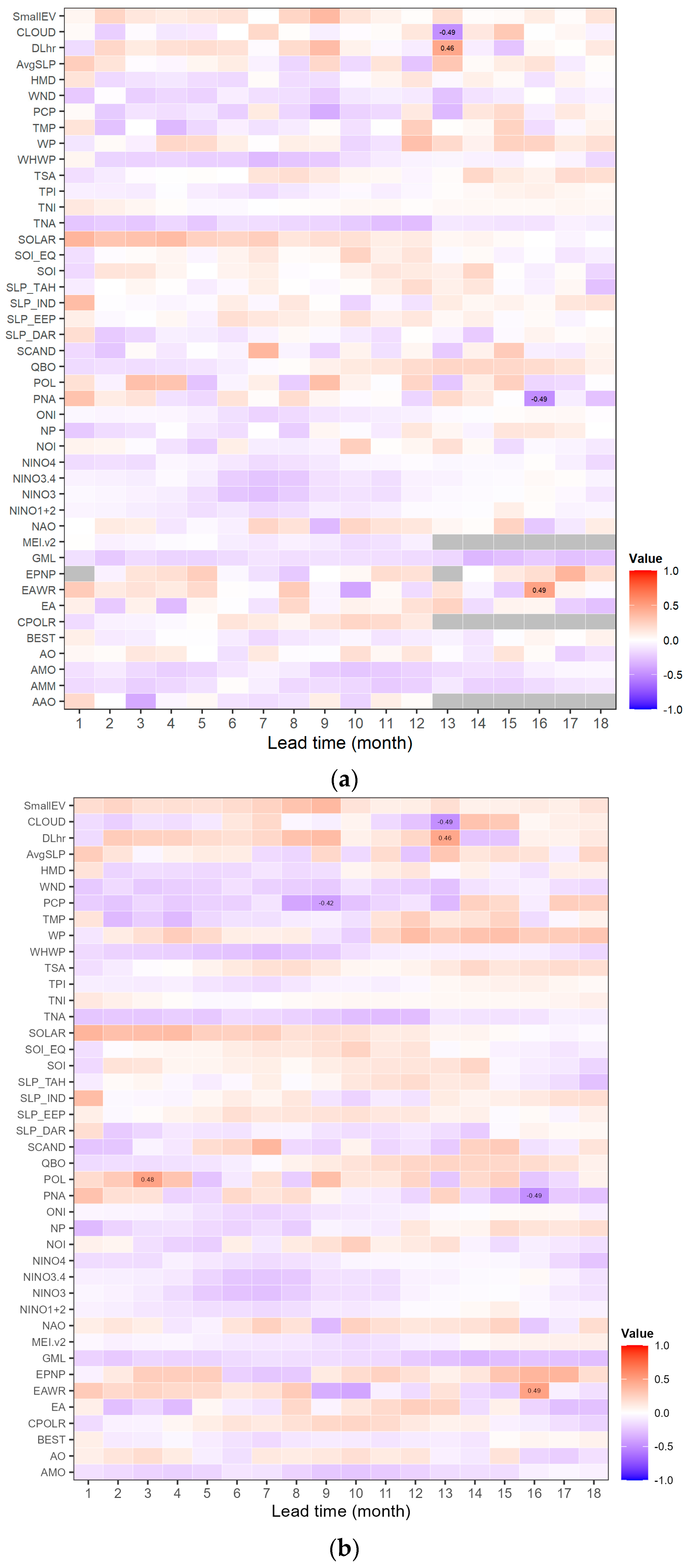
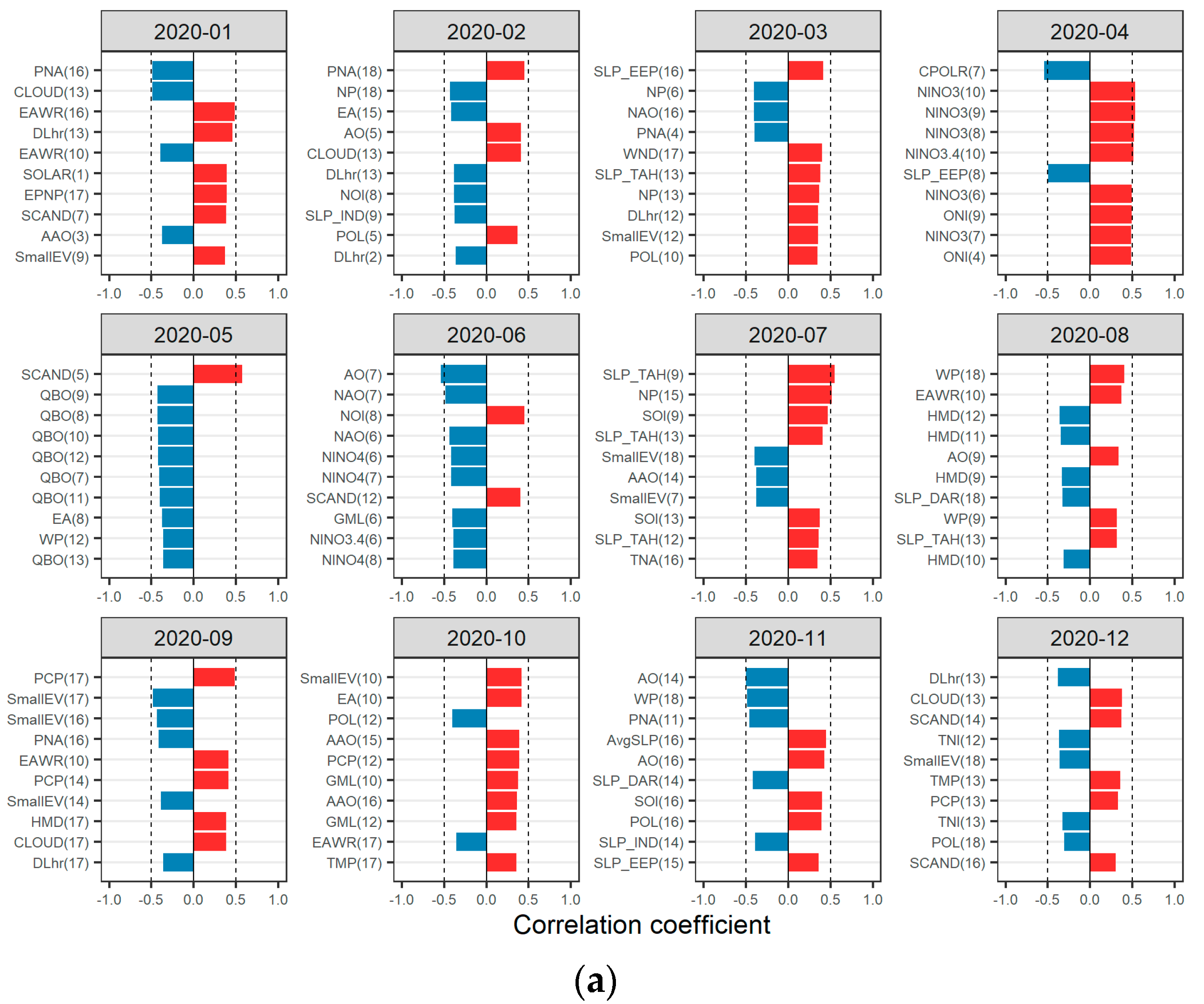
3.1. Teleconnection Analysis

Figure 2 illustrates an example of the teleconnection results with and without considering the duration. The analysis was based on January 2020, where the correlation between January precipitation over the past 40 years (1980–2019) and climate index data for each preceding period (1–18 months) were examined. For instance, the 1-month preceding data for the AAO (Antarctic Oscillation) index corresponds to December data from 1979 to 2018, while the data for an 18-month lead time refers to July data from 1978 to 2017. In Figure 2a, only the month data corresponding to each lead time were analyzed, while Figure 2b shows the correlation results when considering the average values of climate indices for different durations (1, 2, 3 months). Red color indicates positive correlation, blue color indicates negative correlation, and gray color indicates insufficient data for correlation analysis during that period.
For correlations with an absolute value of 0.4 or higher, the results are presented as numerical values. As observed in Figure 2, incorporating the average values of climate indices for up to a maximum of 3 months (Case 2) generally results in higher correlation values. For example, when considering the POL (Polar/Eurasia pattern) index, the correlation with a 3-month lead data is below 0.4 when only the data for the respective month is considered (Case 1), whereas it increases to 0.48 (result for a 2-month duration) when the average values of the climate index for 1 to 3 months are taken into account (Case 2). Incorporating the duration for all analysis periods leads to higher correlation results, even in the case of temperature.
Figure 3 represents the status of climate indices utilized in constructing the prediction models for each month of 2020, with the prediction time point set as December 2019. It displays the top 10 climate indices in terms of correlation coefficient (absolute value) for each month. Figure 3a shows the list of climate indices based on the data for the respective month without considering the duration (Case 1), while Figure 3b presents the list of climate indices with high correlation coefficients obtained by considering the duration of indices (Case 2). In Figure 3a, PNA(16) refers to the 16-month lead data for the PNA index, while in Figure 3b, PNA(16-1) represents the combination of a 16-month lead period and a 1-month duration. In other words, PNA(16) and PNA(16-1) refer to the same data.
In Figure 3, January 2020 corresponds to a 1-month lead, while December 2020 corresponds to a 12-month lead. For the 1-month lead prediction, the range of correlation coefficients for the selected candidate climate indices is −0.491 (maximum) to 0.368 (minimum) based on its values when the duration of the indices is not considered. When the duration is taken into account, the range becomes −0.491 (maximum) to 0.390 (minimum). For the 12-month lead prediction, without considering the duration, the range is −0.384 (maximum) to 0.302 (minimum). However, when the duration is considered, the range is 0.429 (maximum) to 0.348 (minimum). This means that the correlations presented in Figure 3b are higher than those in Figure 3a, and by incorporating the duration of the climate indices, we can utilize indices as predictors that have a higher correlation with the target variable compared to the conventional approach not considering the duration.
During the construction of the forecast model, there are constraints on the available climate indices based on the lead time. However, incorporating the duration expands the range of available predictors with high correlation coefficients. This effect becomes particularly significant as the lead time increases. Therefore, by considering the duration of climate indices, it is possible to identify predictors that exhibit higher correlation with the prediction target (such as precipitation or temperature) not only in the analyzed period but also in other periods.

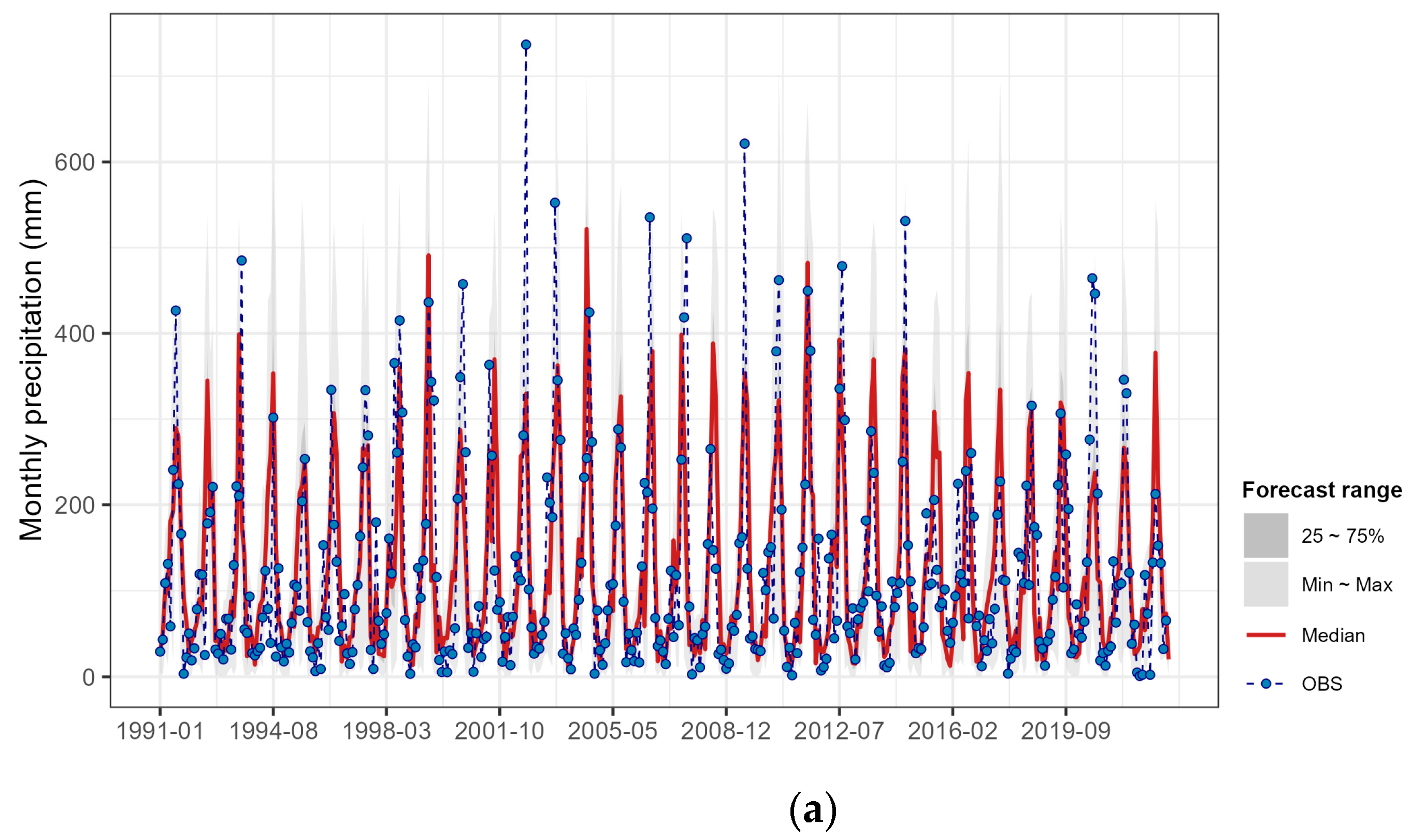
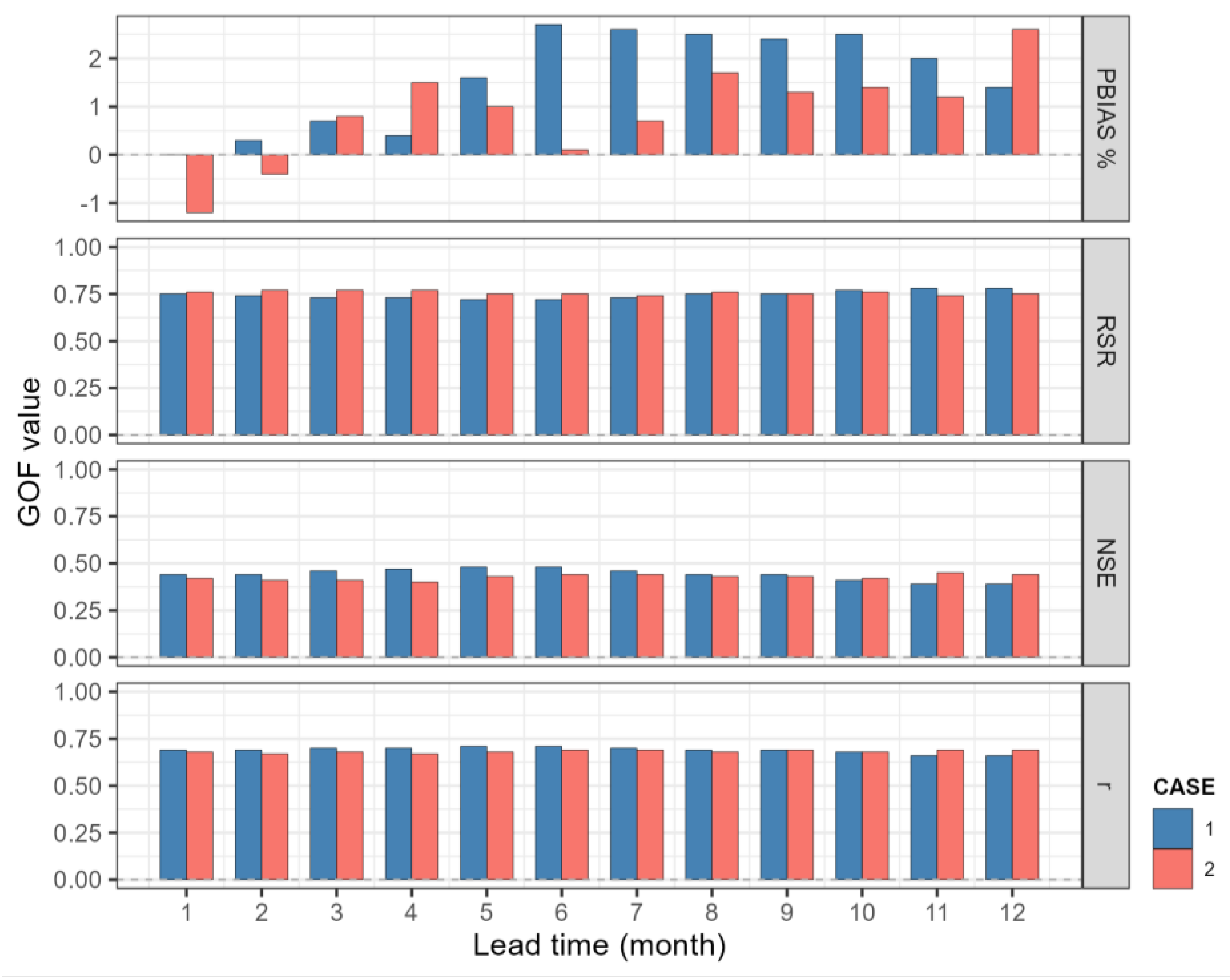
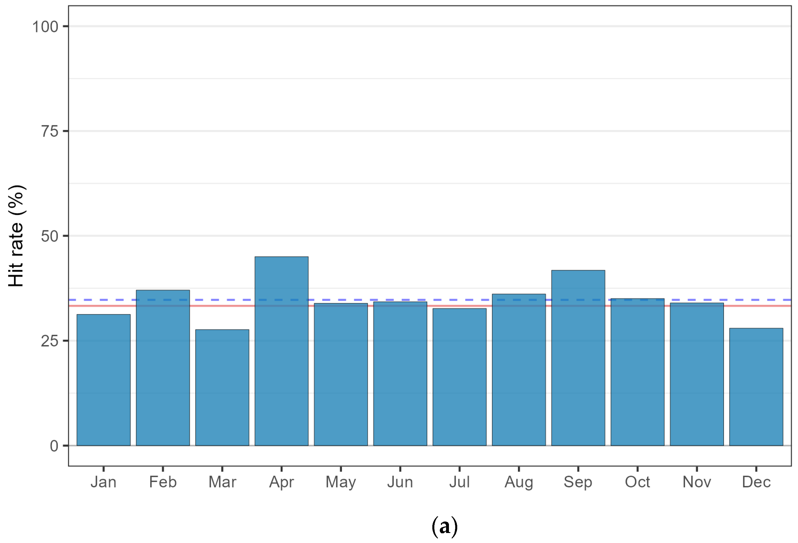
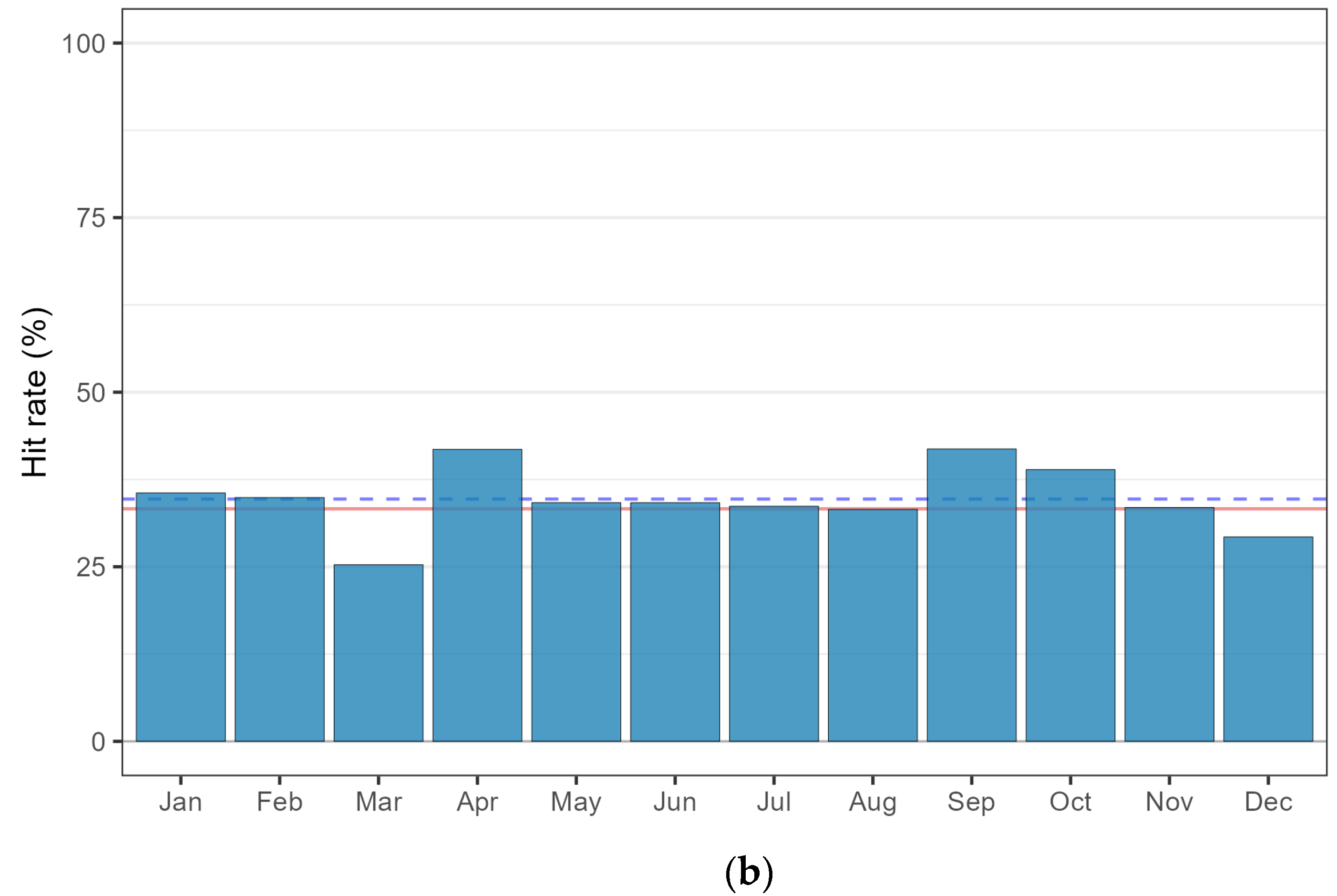
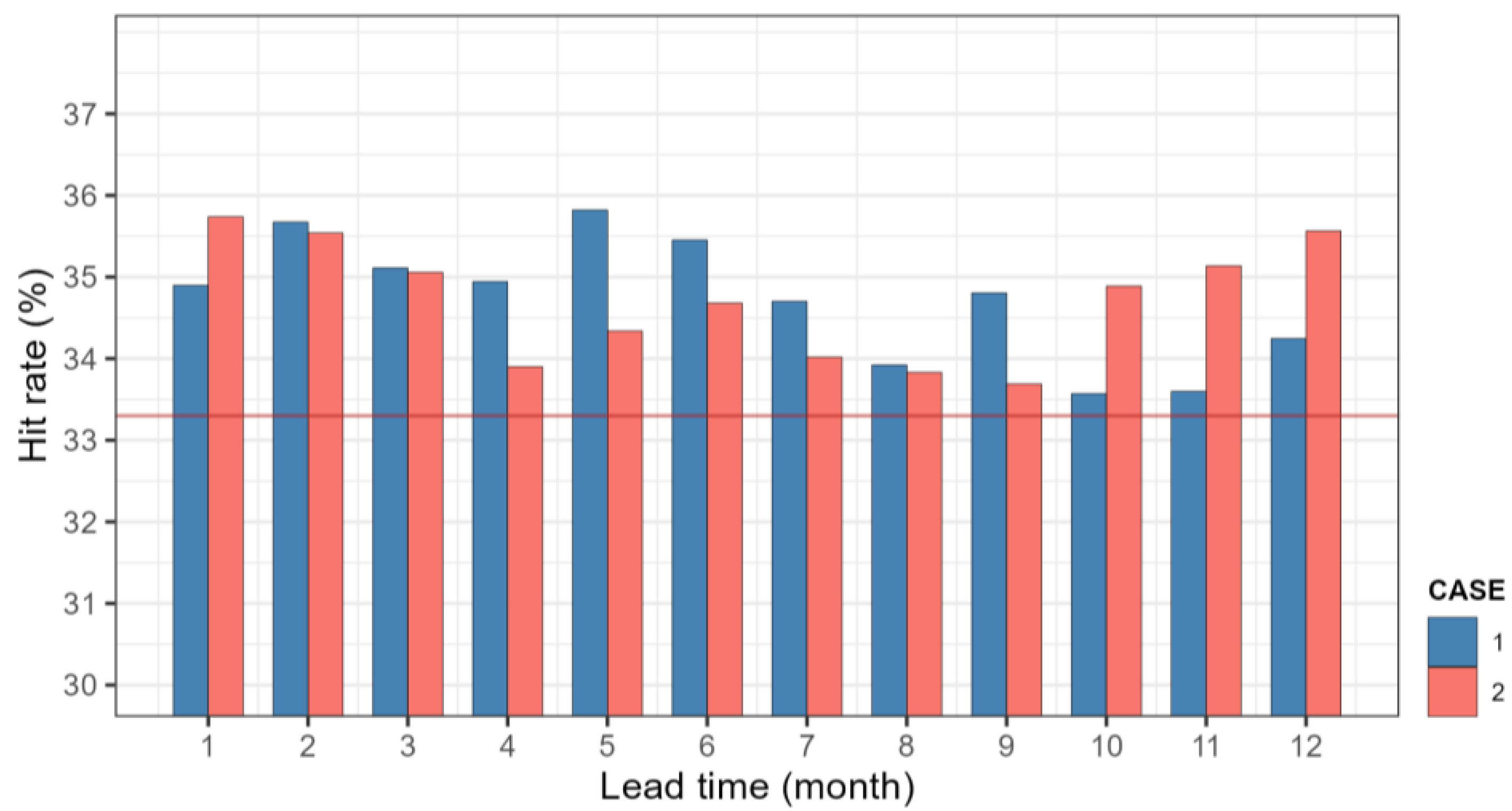
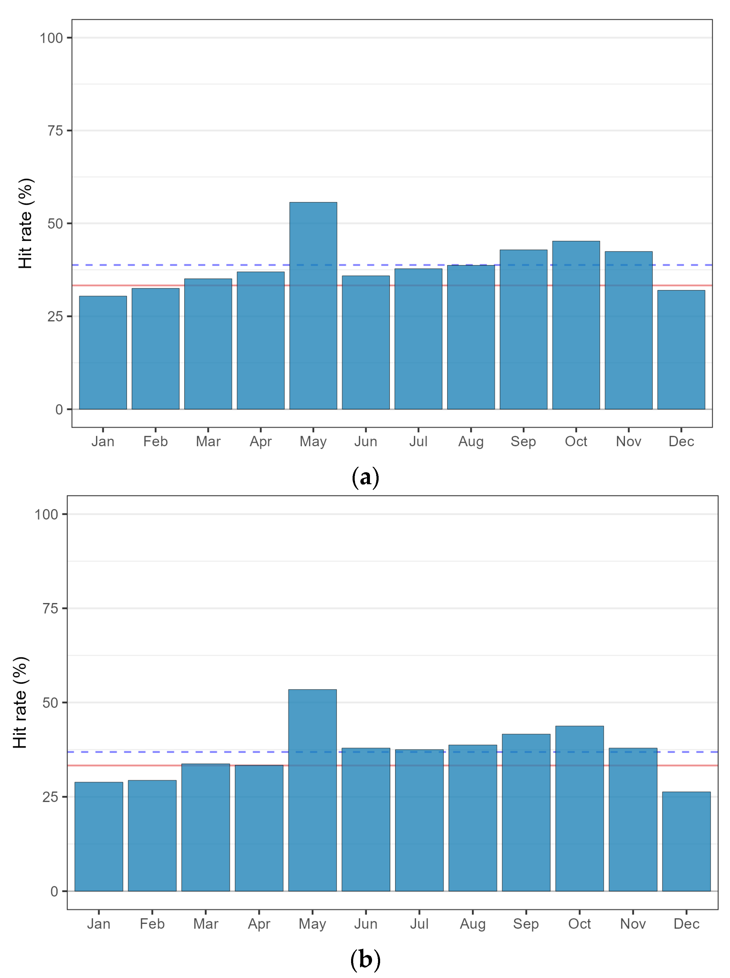
3.2. Precipitation Forecasts

Figure 4 displays a comparison between the predicted monthly rainfall values and the corresponding observed values from January 1991 to December 2022, illustrating the range and median of the predictions. The gray shading represents the prediction range, the red solid line represents the median predicted value, and the blue line represents the observed value. While there may be instances where significant differences between observed and predicted values occur in certain periods, both Figure 4a (without considering the duration of climate indices) and Figure 4b (considering the duration) exhibit similar patterns to the observed values, indicating a seasonal influence.
Figure 5 presents the analysis of the goodness of fit between the average predicted values and observed values for monthly precipitation, considering different prediction lead times ranging from 1 to 12 months. It includes fit indices such as PBIAS, RSR, NSE, and r. Case 1 refers to the scenario where the duration of climate indices is not considered, while Case 2 represents the scenario where the duration is taken into account.
Table 3 provides the range of values for each fit index as presented in Figure 5. Although there may be some variations depending on the lead time, the differences in the values of the fit indices between considering or not considering the duration of climate indices are not substantial. According to the evaluation criteria by Moriasi et al. [23], the PBIAS can be classified as “very good,” while the RSR and NSE are at an “unsatisfactory” level.
As observed in Figure 5, regardless of whether the duration of the predictor is considered or not, PBIAS generally increases with longer lead time. However, when analyzing the values of RSR, NSE, and r, it is observed that for prediction lead times from 1 month to 9 months, the goodness of fit in Case 1 is relatively better. On the other hand, for prediction lead times of 10 months and beyond, the goodness of fit in Case 2 is relatively higher. This suggests that considering the duration of climate indices as a predictor shows potential for enhancing the accuracy of predictions, particularly for longer lead times of 10 months or more.
Figure 6 depicts the analysis of the tercile hit rate for precipitation forecasts. The red color in Figure 6 represents the baseline probability of 33.3%, and the blue dashed line represents the average value for all periods. If the average value is higher than the baseline probability (33.3%), it indicates predictive skill.
As shown in Figure 6, when the duration of the predictive factor is not considered (Case 1), the range of probabilities for each month is 27.6% to 45.0% (average 34.7%). However, when the duration is taken into account (Case 2), the range becomes 25.3% to 41.9% (average 34.7%). Although there may be some monthly differences, the overall results are similar.
Figure 7 displays a bar plot presenting the range of tercile hit rates for each month based on the prediction lead time (1 to 12 months). The red line represents the baseline probability of 33.3%, and values exceeding this threshold indicate meaningful predictive skill. When the duration is not considered, similar to the results in Figure 5, the hit rates decrease after a lead time of 10 months. However, when the duration is taken into account, it is observed that the hit rates for lead times of 10 to 12 months do not drop significantly. The range of hit rate values for lead times of 10 to 12 months is higher when the duration is considered (34.9% to 35.6%) compared to when it is not considered (33.6% to 34.2%). This suggests that incorporating the duration of climate indices as predictors can help maintain higher hit rates for longer lead times, enhancing the accuracy of the tercile-based precipitation forecasts.

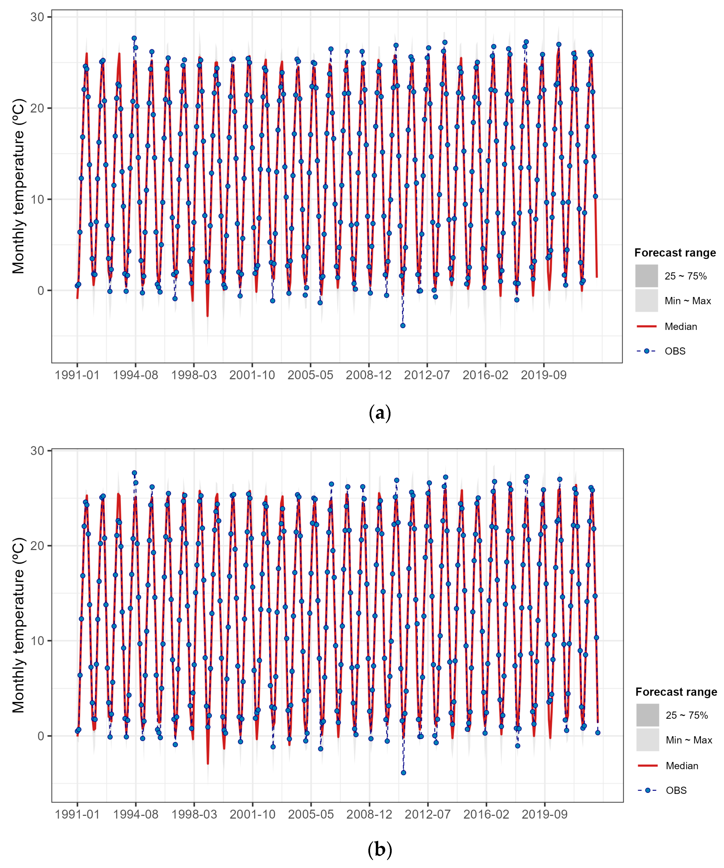
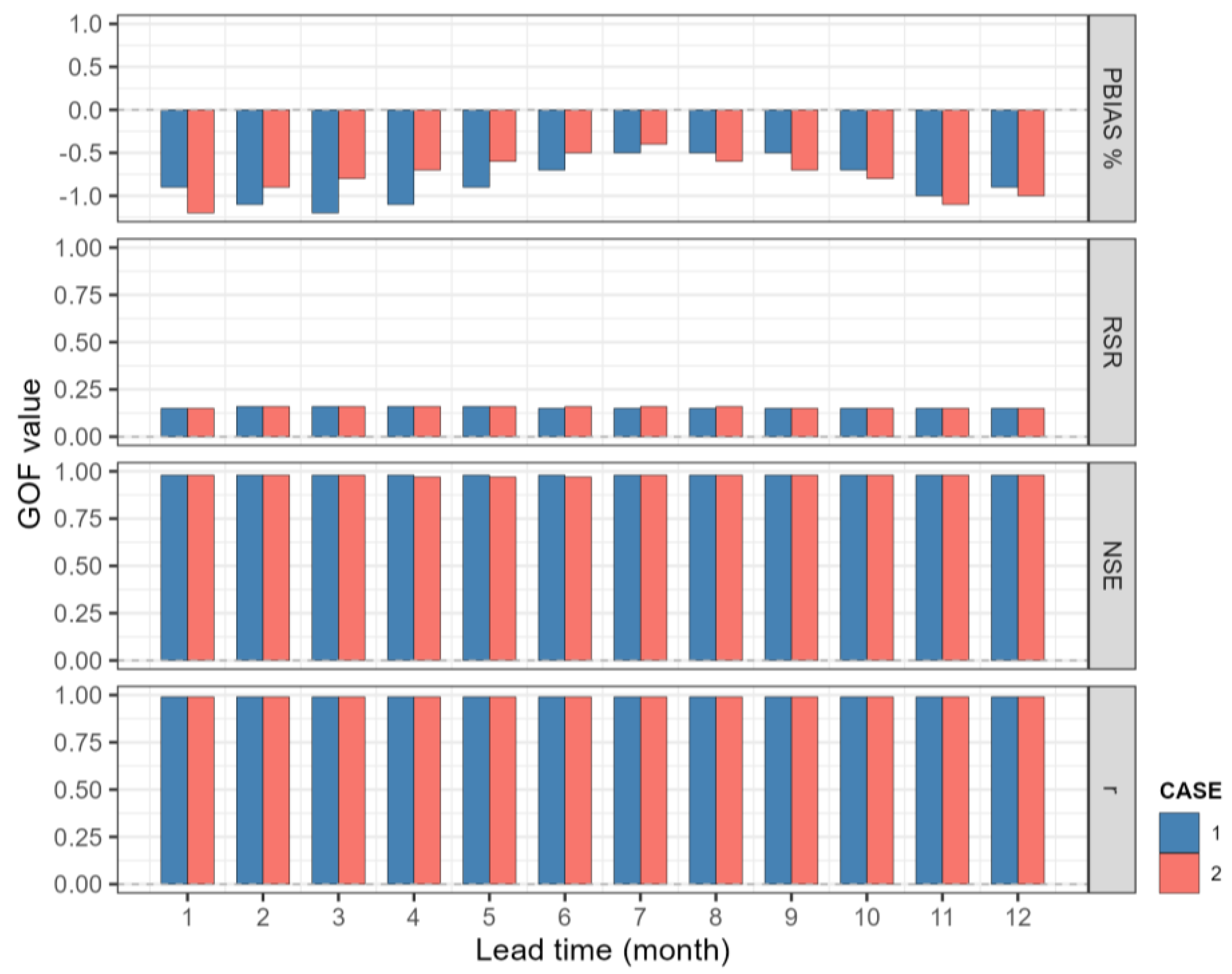
3.3. Temperature Forecasts

Figure 8 illustrates the predicted results for monthly temperatures from 1991 to 2022. Unlike the precipitation forecasts shown in Figure 4, which exhibit some variations depending on the consideration of duration, the temperature predictions show consistent results throughout the entire analysis period. This consistency is further supported by the analysis of goodness of fit presented in Figure 9 and Table 4, where the differences resulting from the consideration of duration are not significant.
Compared to precipitation, the goodness of fit between the predicted results and the actual observed values for temperature is very high, as indicated by the values of PBIAS, RSR, NSE, and r. According to the evaluation criteria by Moriasi et al. [23], PBIAS, RSR, and NSE are considered to be at a very good level. This suggests that the temperature forecasts exhibit a high level of accuracy, regardless of whether the duration of climate indices is considered or not.
Figure 10 presents a comparison of the tercile hit rates for the temperature forecasts on a monthly basis. The case without considering duration yields higher hit rates (ranging from 30.4% to 55.7%, with an average of 38.8%) compared to the case considering duration (ranging from 26.3% to 53.4%, with an average of 36.9%). It was consistently observed that May had the highest hit rate, and the period from May to November generally exhibited relatively higher hit rates. Overall, the average hit rates were higher than the baseline probability of 33.3%, indicating the reliability of the statistically derived temperature forecasts in this study.
Figure 11 illustrates the tercile hit rates for the temperature forecasts across different lead times. It was observed that irrespective of the lead time, the hit rates were higher when the duration of climate indices was not considered. Furthermore, similar to precipitation forecasts, it was noted that for lead times of 10 months or more, the hit rates decrease when duration is not considered, while considering duration improves the hit rates. However, as evident in Figure 8, Figure 9, Figure 10 and Figure 11 and Table 4, there is minimal difference in temperature prediction performance when considering the duration of climatic indices.

4. Discussion

The results obtained from the analysis of precipitation and temperature forecasts provide valuable insights into the predictive performance of the statistical models used in this study.
Regarding precipitation forecasts, Figure 4 demonstrates that both the range and median of the predicted rainfall values exhibit patterns similar to the observed values, indicating a seasonal influence. This suggests that the models capture the general variability of precipitation on a monthly basis. However, it is important to note that there are instances where significant differences between observed and predicted values occur, indicating potential areas for improvement in the models.
The goodness of fit analysis presented in Figure 5 further evaluates the performance of the precipitation forecasts. The fit indices, including PBIAS, RSR, NSE, and r, provide quantitative measures of the agreement between the predicted and observed precipitation values. It is observed that the models generally exhibit a “very good” level of performance according to the evaluation criteria by Moriasi et al. [23] based on PBIAS. However, there is room for improvement as the models show an “unsatisfactory” level of performance based on NSE and RSR. These findings indicate that while the models capture the overall precipitation patterns well, there is room for refinement to enhance the accuracy of predictions. The tercile hit rate analysis presented in Figure 6 and Figure 7 provides insights into the accuracy of tercile-based precipitation forecasts. The results show that considering the duration of climate indices as predictors does not significantly impact the overall tercile hit rates. The average hit rates are relatively consistent between the cases with and without considering duration. However, it is worth noting that the hit rates for lead times of 10 months and beyond are higher when the duration is considered, suggesting that incorporating the duration of climate indices may enhance the accuracy of longer-term precipitation predictions.
Turning to temperature forecasts, Figure 8 demonstrates that the predicted monthly temperature values align well with the observed values throughout the analysis period. This consistency indicates that the models effectively capture the general temperature variations on a monthly basis. The high goodness of fit indicated by PBIAS, RSR, NSE, and r (Figure 9 and Table 4) further supports the notion that the models perform exceptionally well in predicting monthly temperature. The tercile hit rate analysis for temperature forecasts, as shown in Figure 10 and Figure 11, reveals interesting patterns. While the hit rates are generally higher when the duration of climate indices is not considered, the difference is minimal compared to precipitation forecasts. This suggests that the consideration of duration has a limited impact on the accuracy of temperature predictions.
In summary, the results indicate that the statistical models used in this study show promising performance in predicting monthly precipitation and temperature. The models capture the overall patterns and variability of these climatic variables, and the goodness of fit measures demonstrate a high level of agreement between the predicted and observed values. Incorporating the duration of climate indices as predictors shows potential for improving the accuracy of longer-term precipitation forecasts. However, for temperature forecasts, the consideration of duration has a minimal effect on the predictive performance. These findings contribute to the understanding of the predictive capabilities of the statistical models in capturing and forecasting climatic variables, providing valuable information for climate-related decision-making and planning.

5. Conclusions

In this study, long-term weather forecasting using statistical methods was conducted on the Seomjin River basin, and the effects of incorporating the duration of climate indices used as predictive factors were evaluated. The statistical technique utilized in this study was the multiple linear regression model applied in previous studies by Kim et al. [5,6,7]. A total of 44 climate indices, including global climate patterns and local weather factors in the target area, were used as predictive factors. For each target month, the teleconnection analysis of each climate index was performed for different lead times (1–18 months), and the top 10 climate indices with high correlation were selected as candidate predictors. In order to incorporate the duration of climate indices, the correlation analysis was conducted not only for the values of each climate index for the corresponding month, but also for the average values for 2-month and 3-month durations.
The results of the correlation analysis showed that incorporating the duration of climate indices allowed for the selection of climate indices with higher correlation compared to considering only the values for the corresponding month. Particularly, as the forecast lead time increased, the difference in correlation became more pronounced. This indicates that the inclusion of duration in the prediction model expands the range of available climate indices with high correlation, which is important in the process of constructing models where the choice of available predictors is constrained by the forecast lead time.
When comparing the prediction results with and without incorporating the duration, significant differences were observed in precipitation rather than temperature. In precipitation forecasts, incorporating duration maintained a stable tercile hit rate (34.9–35.6%) for lead times of 10–12 months, while excluding duration resulted in a decreased hit rate beyond 10 months (33.6–34.2%). For temperature, hit rates were higher without considering duration. Both precipitation and temperature forecasts had average tercile hit rates above the baseline probability (33.3%) regardless of duration incorporation.
In conclusion, the inclusion of the duration of climate indices as predictive factors in our forecasting models showed the potential to utilize climate indices with higher correlations. This notably improved the predictive skill for precipitation forecasts with lead times of 10–12 months. However, for the overall forecast period, the difference in predictive skill was relatively marginal. As for temperature forecasts, the impact of incorporating the duration on the goodness of fit analysis results was negligible. The influence of incorporating the duration on temperature hit rates will undergo further investigation in future research, encompassing additional applications to different regions.
Furthermore, this study focused solely on the statistical correlation without considering the dynamic relationships between each climate index or between the climate indices and the prediction target. The emphasis was placed on constructing flexible models based on statistical relationships depending on the prediction time. Therefore, due to the limitations of statistical models, predictions may be somewhat compromised for extreme events that differ significantly from historical patterns. However, we anticipate that this issue can be mitigated to some extent by the utilization of new predictive factors and the incorporation of diverse statistical characteristics into the models in the future.

Author Contributions

All authors substantially contributed to the conceiving and designing of the research and realizing this manuscript. Conceptualization and research design, data analysis, C.-G.K.; methodology and validation of results, J.L.; formal analysis and data curation, J.E.L.; funding acquisition and supervision, H.K. All authors have read and agreed to the published version of the manuscript.

Funding

This work was supported by the Korea Environment Industry & Technology Institute (KEITI) through the Water Management Program for Drought Project, funded by the Korea Ministry of Environment (MOE) (2022003610002).

Data Availability Statement

Data is available on request from the authors.

Conflicts of Interest

The authors declare no conflict of interest.

References

  1. White, C.J.; Carlsen, H.; Robertson, A.W.; Klein, R.J.T.; Lazo, J.K.; Kumar, A.; Vitart, F.; Coughlan de Perez, E.; Ray, A.J.; Murray, V.; et al. Potential applications of subseasonal-to-seasonal (S2S) predictions. Meteorol. Appl. 2017, 24, 315–325. [Google Scholar] [CrossRef]
  2. Doblas-Reyes, F.J.; Garcia-Serrano, J.; Lienert, F.; Biescas, A.P.; Rodrigues, L.R.L. Seasonal climate predictability and forecasting: Status and prospects. Wiley Interdiscip. Rev. Clim. Chang. 2013, 4, 245–268. [Google Scholar] [CrossRef]
  3. Schepen, A.; Wang, Q.J.; Robertson, D.E. Combining the strengths of statistical and dynamical modeling approaches for forecasting Australian seasonal rainfall. J. Geophys. Res. 2012, 117, D20107. [Google Scholar] [CrossRef]
  4. Kim, H.-J.; Oh, S.M.; Chung, I.-U. An empirical model approach for seasonal prediction of summer temperature in South Korea. J. Clim. Res. 2018, 13, 17–35. [Google Scholar] [CrossRef]
  5. Kim, C.-G.; Lee, J.; Lee, J.E.; Kim, N.W.; Kim, H. Monthly precipitation forecasting in the Han River basin, South Korea, using large-scale teleconnections and multiple regression models. Water 2020, 12, 1590. [Google Scholar] [CrossRef]
  6. Kim, C.-G.; Lee, J.; Lee, J.E.; Kim, N.W.; Kim, H. Monthly temperature forecasting using large-scale climate teleconnections and multiple regression models. J. Korea Water Resour. Assoc. 2021, 54, 731–745. [Google Scholar]
  7. Kim, C.-G.; Lee, J.; Lee, J.E.; Kim, H. Application of multiple linear regression and artificial neural network models to forecast long-term precipitation in the Geum River basin. J. Korea Water Resour. Assoc. 2022, 55, 723–736. [Google Scholar]
  8. Feng, P.; Wang, B.; Liu, D.L.; Ji, F.; Niu, X.; Ruan, H.; Shi, L.; Yu, Q. Machine learning-based integration of large-scale climate drivers can improve the forecast of seasonal rainfall probability in Australia. Environ. Res. Lett. 2020, 15, 084051. [Google Scholar] [CrossRef]
  9. Kang, B.; Lee, B. Application of artificial neural network to improve quantitative precipitation forecasts of meso-scale numerical weather prediction. J. Korea Water Resour. Assoc. 2011, 44, 97–107. [Google Scholar] [CrossRef]
  10. Lee, K.-J.; Kwon, M. A prediction of precipitation over East Asia for June using simultaneous and lagged teleconnection. Atmosphere 2016, 26, 711–716. [Google Scholar] [CrossRef]
  11. Kim, M.-K.; Kim, H.-S.; Kwak, C.-H.; So, S.-S.; Suh, M.-S.; Park, C.-K. Long-term forecast of seasonal precipitation in Korea using the large-scale predictors. J. Korean Earth Sci. Soc. 2002, 23, 587–596. [Google Scholar]
  12. Kim, H.-S. Seasonal precipitation forecast in the Korean Peninsula using delay-correlated large-scale predictors. Atmosphere 2002, 12, 133–136. [Google Scholar]
  13. Kim, M.-K.; Kim, Y.-H.; Lee, W.-S. Seasonal prediction of Korean regional climate from preceding large-scale climate indices. Int. J. Climatol. 2007, 27, 925–934. [Google Scholar] [CrossRef]
  14. Hwang, Y.-J.; Ahn, J.-B. A correlation of East Asian summer precipitation simulated by PNU/CME CGCM using multiple linear regression. J. Korean Earth Sci. Soc. 2007, 28, 214–226. [Google Scholar] [CrossRef]
  15. Kwon, M.; Lee, K.-J. A prediction of Northeast Asian summer precipitation using the NCEP climate forecast system and canonical correlation analysis. J. Korean Earth Sci. Soc. 2014, 35, 88–94. [Google Scholar] [CrossRef]
  16. Jo, S.; Ahn, J.-B. Statistical forecast of early spring precipitation over South Korea using multiple linear regression. J. Clim. Res. 2017, 12, 53–71. [Google Scholar] [CrossRef]
  17. Park, M.-G.; Kang, S.-U.; Lee, J.-J.; Lee, H.-H.; Kim, H.-J. Seasonal precipitation forecast using big data. Mag. Korea Water Resour. Assoc. 2018, 51, 6–12. [Google Scholar]
  18. Han, B.-R.; Lim, Y.; Kim, H.-J.; Son, S.-Y. Development and evaluation of statistical prediction model of monthly-mean winter surface air temperature in Korea. Atmosphere 2018, 28, 153–162. [Google Scholar]
  19. Yoo, C.; Johnson, N.C.; Chang, C.-H.; Feldstein, S.B.; Kim, Y.-H. Subseasonal prediction of wintertime East Asia temperature based on atmospheric teleconnections. J. Clim. 2018, 31, 9351–9366. [Google Scholar] [CrossRef]
  20. Jung, J.; Kim, H.S. Predicting temperature and precipitation during the flood season based on teleconnection. Geosci. Lett. 2022, 9, 4. [Google Scholar] [CrossRef]
  21. Lee, Y.; Kim, H.-R.; Noh, N.; Kim, K.-Y.; Kim, B.-M. Enhancing forecast skill of winter temperature of East Asia using teleconnection patterns simulated by GloSea5 seasonal forecast model. Atmosphere 2023, 14, 438. [Google Scholar] [CrossRef]
  22. Kwon, M. Development of Seasonal Prediction Models for East Asian Summer Monsoon/Changma; Korea Institute of Ocean Science & Technology: Busan, Republic of Korea, 2015; CATER 2012-3070. [Google Scholar]
  23. Moriasi, D.N.; Arnold, J.G.; Liew, M.W.; Bingner, R.L.; Harmel, R.D.; Veith, T.L. Model evaluation guidelines for systematic quantification of accuracy in watershed simulations. Trans. ASABE 2007, 50, 885–900. [Google Scholar] [CrossRef]
Figure 1. Study area.
Water 15 03291 g001
Figure 2. Results of teleconnection analysis between historical precipitation data and each climate index data by lead time based on January 2020: (a) Case 1. Not considering the duration of climate indices; (b) Case 2. Considering the duration of climate indices.
Water 15 03291 g002
Figure 3. Status of climate indices utilized in the models forecasting monthly precipitation for the year of 2020: (a) Case 1. Not considering the duration of climate indices; (b) Case 2. Considering the duration of climate indices. The numbers in parentheses in Case 1 (a) indicate the lead time (months) from the target month, and in Case 2 (b), the first number represents the lead time, and the second number represents the duration of the climate indices. The blue bars indicate negative correlation values, while the red bars signify positive correlation values.
Water 15 03291 g003aWater 15 03291 g003b
Figure 4. Results of precipitation forecasts from 1991 to 2022: (a) Case 1. Not considering the duration of climate indices; (b) Case 2. Considering the duration of climate indices.
Water 15 03291 g004aWater 15 03291 g004b
Figure 5. Goodness of fit analysis of monthly precipitation forecasts according to the lead time.
Water 15 03291 g005
Figure 6. Tercile hit rate for monthly precipitation forecasts: (a) Case 1. Not considering the duration of climate indices; (b) Case 2. Considering the duration of climate indices. The red solid line represents the baseline probability of 33.3%, and the blue dashed line represents the average value for all months.
Water 15 03291 g006aWater 15 03291 g006b
Figure 7. Tercile hit rate for precipitation forecasts according to the lead time. The red line represents the baseline probability of 33.3%.
Water 15 03291 g007
Figure 8. Results of temperature forecasts from 1991 to 2022: (a) Case 1. Not considering the duration of climate indices; (b) Case 2. Considering the duration of climate indices.
Water 15 03291 g008
Figure 9. Goodness of fit analysis of monthly temperature forecasts according to the lead time.
Water 15 03291 g009
Figure 10. Tercile hit rate for monthly temperature forecasts: (a) Case 1. Not considering the duration of climate indices; (b) Case 2. Considering the duration of climate indices. The red solid line represents the baseline probability of 33.3%, and the blue dashed line represents the average value for all months.
Water 15 03291 g010
Figure 11. Tercile hit rate for temperature forecasts according to the lead time. The red line represents the baseline probability of 33.3%.
Water 15 03291 g011
Table 1. ASOS stations used in this study.
IDStation NameLatitude (°N)Longitude (°E)Elevation (m a.s.l)
146Jeonju35.84127.1261.40
156Gwangju35.17126.8972.38
168Yeosu34.74127.7464.64
170Wando34.40126.7035.24
174Suncheon35.02127.37165.00
244Imsil35.61127.29247.04
245Jeongeup35.56126.8469.84
247Namwon35.42127.40132.50
248Jangsu35.66127.52406.49
254Sunchanggun35.37127.13127.00
256Juam35.08127.2474.63
258Boseonggun34.76127.212.80
259Gangjingun34.63126.7712.50
260Jangheung34.69126.9245.02
261Haenam34.55126.5716.36
262Goheung34.62127.2851.91
266Gwangyangsi34.94127.6986.70
289Sancheong35.41127.88138.07
Table 2. Predictors used in this study [5,6,7].
PredictorDescriptionProvider
Global climate indexAAOAntarctic oscillationNOAA
AMMAtlantic meridional modeNOAA
AMOAtlantic multidecadal oscillationNOAA
AOArctic oscillationNOAA
BESTBivariate ENSO timeseriesNOAA
CPOLRMonthly central Pacific outgoing long wave radiation index (170E–140W, 5S–5N)NOAA
EAEast Atlantic patternNOAA
EAWREast Atlantic/Western Russia patternNOAA
EPNPEast Pacific/North Pacific oscillationNOAA
GMLGlobal mean land-ocean temperature indexNOAA
MEI.v2Multivariate ENSO index version 2NOAA
NAONorth Atlantic oscillationNOAA
NINO1+2Extreme eastern tropical Pacific SST (0–10S, 90W–80W)NOAA
NINO3Eastern tropical Pacific SST (5N–5S, 150W–90W)NOAA
NINO3.4East central tropical Pacific SST (5N–5S, 170–120W)NOAA
NINO4Central tropical Pacific SST (5N–5S, 160E–150W)NOAA
NOINorthern oscillation indexNOAA
NPNorth Pacific patternNOAA
ONIOceanic Niño indexNOAA
PNAPacific American indexNOAA
POLPolar/Eurasia patternNOAA
QBOQuasi-biennial oscillationNOAA
SCANDScandinavia patternNOAA
SLP_DARDarwin sea level pressNOAA
SLP_EEPEquatorial eastern Pacific sea level pressNOAA
SLP_INDIndonesia sea level pressNOAA
SLP_TAHTahiti sea level pressNOAA
SOISouthern oscillation indexNOAA
SOI_EQEquatorial SOINOAA
SOLARSolar flux (10.7 cm)NOAA
TNATropical northern Atlantic indexNOAA
TNITrans-Niño indexNOAA
TPITripole index for the interdecadal Pacific oscillationNOAA
TSATropical southern Atlantic indexNOAA
WHWPWestern hemisphere warm poolNOAA
WPWestern Pacific indexNOAA
Local climate indexPCPMonthly precipitationKMA
TMPMonthly average temperatureKMA
HMDMonthly average relative humidityKMA
AvgSLPMonthly average sea level pressureKMA
DLhrMonthly sum of daylight hoursKMA
WNDMonthly average wind speedKMA
CLOUDMonthly average cloud coverKMA
SmallEVMonthly sum of small pan evaporationKMA
Table 3. Goodness of fit analysis results for precipitation forecasts.
PBIASRSRNSEr
Case 10~+2.7%0.72~0.780.39~0.480.66~0.71
Case 2−1.2~+2.6%0.74~0.770.40~0.450.67~0.69
Table 4. Goodness of fit analysis results for temperature forecasts.
PBIASRSRNSEr
Case 1−1.2~−0.5%0.15~0.160.980.99
Case 2−1.2~−0.4%0.15~0.160.97~0.980.99
Disclaimer/Publisher’s Note: The statements, opinions and data contained in all publications are solely those of the individual author(s) and contributor(s) and not of MDPI and/or the editor(s). MDPI and/or the editor(s) disclaim responsibility for any injury to people or property resulting from any ideas, methods, instructions or products referred to in the content.

