Article

A Novel Intelligent Model for Monthly Streamflow Prediction Using Similarity-Derived Method

1
School of Civil and Hydraulic Engineering, Huazhong University of Science and Technology, 1037 Luoyu Road, Wuhan 430074, China
2
Institute of Product Quality Standards in Ministry of Water Resources, 19 Zhuantang Science and Technology Economic Park, Xihu District, Hangzhou 310030, China
3
School of Engineering and Built Environment, Griffith University, Gold Coast Campus, Southport, QLD 4222, Australia
4
Institute of Water Resources and Hydropower, Huazhong University of Science and Technology, 1037 Luoyu Road, Wuhan 430074, China
*
Author to whom correspondence should be addressed.
Water 2023, 15(18), 3270; https://doi.org/10.3390/w15183270
Submission received: 15 August 2023 / Revised: 4 September 2023 / Accepted: 13 September 2023 / Published: 15 September 2023

Abstract

:
Accurate monthly streamflow prediction is crucial for effective flood mitigation and water resource management. The present study proposes an innovative similarity-derived model (SDM), developed based on the observation that similar monthly streamflow patterns recur across different years under comparable hydrological and climate conditions. The model is applied to the Lancang River Basin in China. The model performance is compared with the commonly used support vector machine (SVM) and Mean methods. Evaluation measures such as RMSE, MAPE, and NSE confirm that SDM6 with a reference period of six months achieves the best performance, improving the Mean model by 79.9 m3/s in RMSE, 6.07% in MAPE, and 8.62% in NSE, and the SVM by 53.65 m3/s, 0.24%, and 5.53%, respectively.

1. Introduction

Streamflow prediction, especially in a long-term context, is vital in preventing or mitigating floods and optimizing water resource allocation and reservoir operations [1]. The streamflow process is well known to be influenced by several known factors, including precipitation, evaporation, and temperature, alongside various unknown factors. As a result, streamflow time series tend to be nonlinear, time-varying, and uncertain [2,3,4]. Moreover, the underlying mechanisms of a streamflow process vary significantly during periods of low, moderate, and high flow, particularly during extreme events [5]. Accurate and consistent streamflow prediction presents a challenging task, necessitating developing and utilizing robust and reliable techniques [6,7].
Over the past few decades, numerous streamflow prediction models have been developed, primarily categorized into process-driven and data-driven models [8]. Process-driven modeling methods are considered helpful in ecohydrology, land–atmosphere coupling [9,10], and providing predictions under non-stationary climate conditions, as well as for land use or land cover changes [11]. They have become increasingly important in situations involving short-term predictions of geomorphic hazards, flood dynamics, and complex feedback mechanisms (such as land–atmosphere coupling) [12,13,14] but require complex mathematical models, accurate knowledge of the physical processes of streamflow formation, large amounts of hydrological and meteorological data, and sometimes human judgment [15,16]. Applying these models is constrained by various factors, which can result in poor predictive performance and inherent uncertainties.
However, despite the inherently stochastic characteristics of hydrological processes, there is a burgeoning field of research dedicated to developing models capable of effectively characterizing these complex phenomena. Data-driven models are extensively employed in prediction tasks to fulfill the demands of high accuracy and reliability, particularly in hydropower plant and reservoir operation and management, where long-term scheduling heavily relies on monthly streamflow predictions [17].
Numerous studies have been dedicated to streamflow forecasting using time-series models, with notable examples including the autoregressive integrated moving average (ARIMA) model [18], as well as MA and AR models [19]. While these models often assume a linear relationship between inputs and outputs, the actual relationship is typically characterized by a higher degree of nonlinearity. Artificial neural networks (ANNs), recognized for their robust nonlinear mapping capabilities, have been successfully applied in various fields, including hydrology and water resources, due to their ability to capture complex relationships [20,21]. With the advancement of intelligent algorithms, many other intelligent methods have been utilized for streamflow prediction [22,23]. Chang et al. [24], for instance, applied a fuzzy neural network (CFNN) that can automatically generate rules for clustering the input data. Ni et al. [25] showcased a Genetic-Programming (GP) model for annual streamflow prediction, highlighting its potential as an alternative tool. Zhan et al. [26] introduced a variational Bayesian neural network (VBNN) model for ensemble flood forecasting, revealing its superior performance in liability over the other comparable models. Hu et al. [27] applied an ANN and long short-term memory (LSTM) network models to simulate rainfall–streamflow processes in flood events, demonstrating that LSTM exhibits superior stability and intelligence compared to ANNs. Zhao et al. [28] also demonstrated that the least squares support vector machine (LSSVM) performs well when applied to streamflow prediction. However, these intelligent methods exhibit limitations such as slow learning speed, overfitting, and the curse of dimensionality. A dynamically driven recurrent neural network (RNN) was proposed by Coulibaly and Baldwin [29] to directly forecast hydrological time series, which was proved to be a good alternative for the modeling of the complex dynamics of a hydrological system. Chu et al. [30] developed a classification-based deep belief network (DBN) to improve the performance of data-driven models in streamflow forecasting by integrating physical processes. Danandeh et al. [31] proposed Pareto-optimal moving average multigene genetic programming (MA-MGGP) to develop a parsimonious model for single-station streamflow prediction, which exhibits a noteworthy importance in being applied in practice.
In this study, a novel similarity-derived model (SDM) based on the observation that similar monthly streamflow patterns recur across different years under comparable hydrological and climate conditions is proposed, which can then be utilized to forecast monthly streamflow. The SDM is a data-driven model based on historical patterns. Through the analysis of historical hydrological data, it is evident that the deterministic variations in hydrological phenomena manifest as annual cyclic changes, while hydrological processes within the same watershed display statistical similarity and are influenced by meteorological factors. Similarly, Thomas and Fiering [32] described a linear stochastic model for simulating synthetic flow data, which also incorporates the concept of runoff similarity. However, a key distinction is that this model is linear and employs monthly continuous similarity, whereas the SDM is grounded in interannual similarity, addressing two quadratic problems. Comparable to ANNs and other intelligent algorithms, SDM employs multiple iterative optimizations during the parameter calibration process to maintain the desired objectives. The distinctive feature, however, lies in its approach to prediction, where it utilizes a time-series linear weighted method for computation. In sum, this model represents a synthesis of intelligent algorithms and traditional linear methods for problem resolution.
The present SDM involves tasks to (1) create a two-step model that consists of a similarity parameter calibration model and a similarity derivation prediction model that capture and utilize the observed similarity patterns; (2) re-sequence the historical streamflow and rainfall datasets and divide them into three segments for evaluation; (3) calibrate the reference period length parameter of the SDM using the dataset and validate it using the independent validation set; and (4) assess the predictive accuracy of the SDM by comparing it with Support Vector Machines (SVM) and Mean Annual Average Streamflow.
In the remainder of this paper, Section 2 presents the data processing details and introduces the two-step model that includes the similarity parameter calculation and derivation models and two methods for comparison. Section 3 provides a comprehensive overview of the study area and characteristics of the data, presents the calibration process of parameters using the verification set, and compares the forecast results with other models, followed by a discussion. Finally, Section 4 concludes the research and summarizes the key findings.

2. Problem Formulation and Solution Techniques

2.1. Data Processing

Traditionally, annual natural streamflow data are used as the input in prediction models without altering their original order, but the prediction model proposed in this paper requires preprocessing the streamflow data sequence. Similarly, this processing is applied to the rainfall series.
Figure 1 illustrates the procedure for processing the original streamflow data using the streamflow from consecutive years. As shown in the figure, the consecutive monthly streamflow over multiple years is rearranged into sequences of equal length, with a designated forecast-start month (m) as the reference point to divide each sequence into two parts, the reference and forecast periods, consisting of M _ months preceding and M ¯ months following the forecast-start month (m), respectively. The introduction of the prediction model that follows will be based on the rearranged streamflow sequences.

2.2. Similarity Parameters

The similarity derivation model is based on the correlation of the monthly streamflow processes between the reference and forecast periods, aiming to maximize the linear relationship of similarity between the two periods, which is equivalent to minimizing the difference of similarity measurement, expressed mathematically as:
min λ t , β t , a , b i = 1 N [ F i ( a F ^ i + b ) ] 2
where, N is the number of monthly streamflow sequences rearranged; sequences of monthly streamflow are all paired and indexed for i = 1, 2, …, N; a and b are coefficients to be estimated; and F ^ i and F i represent the weighted similarity measurement of the ith pair of sequences during the forecast period and the whole sequence, respectively, with
F i = t = m M _ m + M ¯ 1 λ t ( Q t ( y 1 ( i ) ) Q t ( y 2 ( i ) ) ) 2 + β t ( P t ( y 1 ( i ) ) P t ( y 2 ( i ) ) ) 2 , [ y 1 ( i ) y 2 ( i ) ]
F ^ i = t = m m + M ¯ 1 [ Q t ( y 1 ( i ) ) Q t ( y 2 ( i ) ) ] 2 , [ y 1 ( i ) y 2 ( i ) ]
where, m is the forecast-start month; M ¯ and M _ represent the number of months in the forecast and reference periods, respectively; the ith pair has two sequences, y1(i) and y2(i) (any combination of non-equal years in the sequences); and λ t   and   β t are the weights assigned to the variance of streamflow ( Q t ( y ) ) and rainfall ( P t ( y ) ) in month t, respectively, and they also serve to standardize the units of streamflow and rainfall.
The parameters are calibrated subject to the following:
1.
The base magnitude assigned to streamflow, being no more than 1.0:
λ t 1.0
2.
Zero-weights assigned to streamflow unknown in the forecast period:
λ t = 0 ,   for   m t m + M ¯ 1
3.
Zero-weights assigned to rainfalls unavailable in the forecast period:
β t = 0 ,   for   m t m + M ¯ 1
For the optimization problem (1)–(6), it is typically quadratic programming (QP) that gives the optimums: a , b , λ t   and   β t .

2.3. Similarity Derivation Model

The monthly streamflow to be predicted, denoted as Q ^ i ( 0 ) , is derived as a weighted value of streamflow from the years that present the highest similarity to the current year,
Q ^ t ( 0 ) = y = 1 Y [ μ y Q t ( y ) ]   for   t = m , m + 1 , , m + M ¯ 1
where, μ y is the weight to be calibrated and assigned to the yth year among the Y most similar years, which will be selected among all historical years based on the similarity measurement during the reference months:
F k = t = m M _ m 1 λ t ( Q t ( k ) Q t ( 0 ) ) 2 + β t ( P t ( k ) P t ( 0 ) ) 2
in which Q t ( 0 ) and Q t ( k ) are streamflow in month y in the current year and the kth year among all historical years, respectively; P t ( 0 ) and P t ( k ) are rainfalls in month y in the current year and the kth year, respectively; A smaller value of (Fk) indicates a higher similarity of the kth year to the current year.
The weights ( μ y ) are calibrated to maximize the similarity of the weighted sequence to the current year during the reference months:
min μ y t = m M _ m 1 λ t ( Q ^ t Q t ( 0 ) ) 2 + β t ( P ^ t P t ( 0 ) ) 2
with the weighted streamflow and rainfall sequences determined as
Q ^ t = y = 1 Y [ μ y Q t ( y ) ] P ^ t = y = 1 Y [ μ y P t ( y ) ]
and the weights interpreted as the contribution ratio from each year,
y = 1 Y μ y = 1.0
The optimization involving (9)–(11) is also a QP problem that can be easily solved with a commercial solver to determine the optimum: μ y .
The SDM introduces two quadratic programming (QP) problems, both of which require solvers for resolution. The first QP problem, the construction objective of the similarity parameter model, aims to optimize the weighting coefficients for runoff and rainfall. The second QP problem, about the similarity-derived model, is focused on predicting the monthly runoff for specified months. The approach to solving the model involves first optimizing the weight parameters. Subsequently, these weight parameters are used to construct the prediction model. The prediction model is then employed for rolling calculations to produce long sequences of monthly runoff predictions.

2.4. Brief Introduction of the Methods for Comparison

This work validates the predictive accuracy by comparing the SDM with two other methods, the SVM and Mean method.
Developed by Vapnik [33], SVM is recognized as one of the most effective tools in prediction fields. Unlike traditional machine learning methods, SVM is based on statistical learning theory and utilizes a kernel function to transform complex nonlinear problems into linear ones in a higher-dimensional space, simplifying the problem-solving process. The main idea behind SVM is to establish a classification hyperplane as the decision boundary, aiming to maximize the margin of separation between positive cases and counterexamples.
Monthly mean runoffs serve as an essential indicator of the long-term streamflow trend in a watershed, offering valuable information for water resources management, particularly in small watersheds with incomplete data, and are commonly utilized for initial estimation in streamflow prediction and used as comparison methods [34].

3. Case Studies

3.1. Research Domain and Data

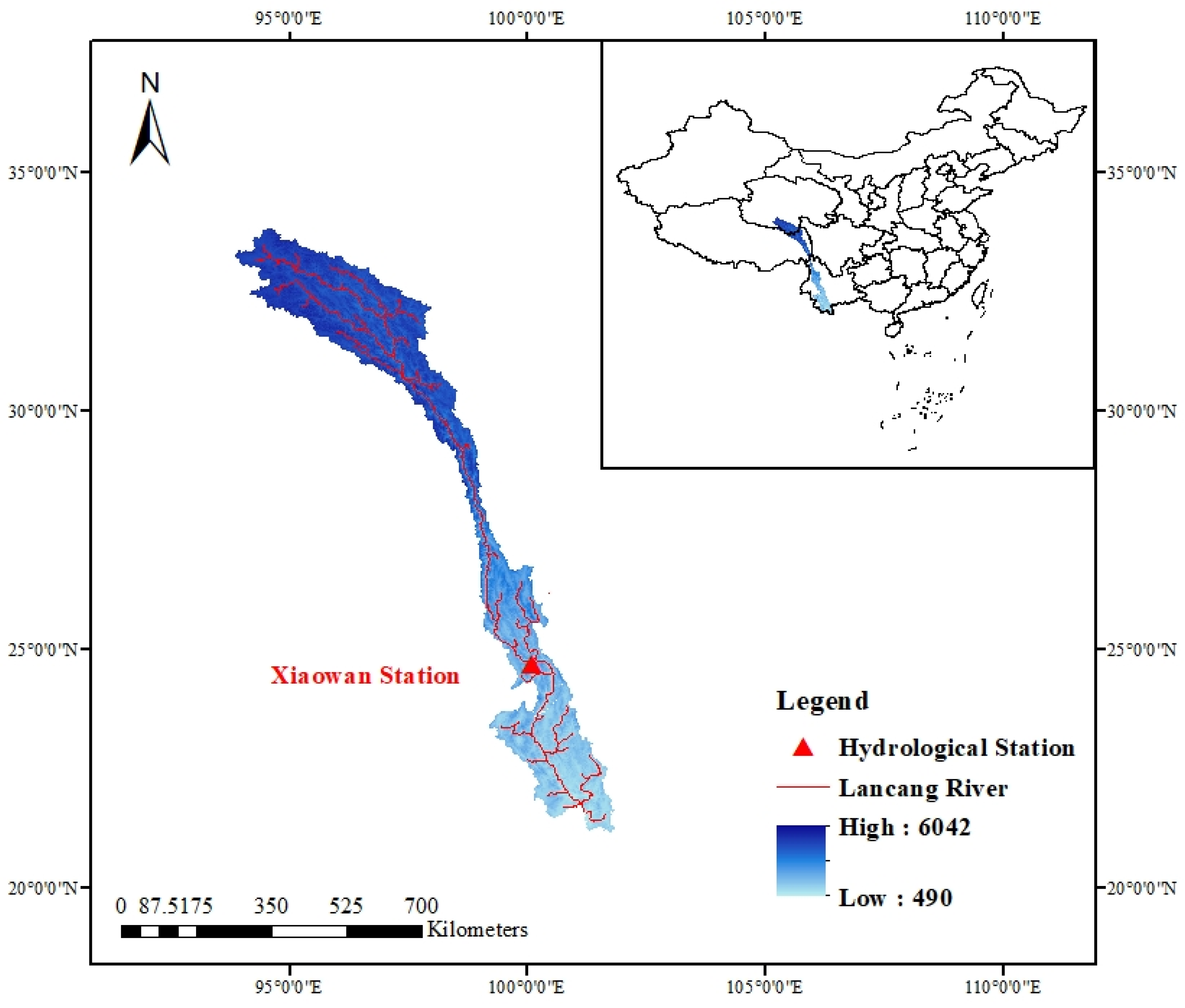
The model and solution presented in this work were applied to the Lancang River basin, as shown in Figure 2, which, located between 21°30′ N and 32°40′ N latitude and 94° E to 101°50′ E longitude, is part of the Lancang–Mekong River system, originating from the northeastern part of Tanggula Mountain in Qinghai Province, China. The river flows through Myanmar, Laos, Thailand, and Cambodia before reaching its mouth at the South China Sea in Ho Chi Minh City, Vietnam, making it the largest international river in Southeast Asia, with a length of 4880 km and a drainage area of 826,200 km2 [35]. The Lancang River in China is known for its mainstream length of 2161 km and drainage area of 167,487 km2. The Lancang River, traversing the Hengduan Mountains, is characterized by its north–south orientation and is separated from the Nujiang River in the west by mountain ranges such as Bangma Mountain and Nushan, including the southern part of Luoxue Mountain, and the Jinsha River and Red River in the east by mountain ranges such as Yun Ling and Wu Liangshan [36]. Significant natural environmental differences exist between the river’s upper, middle, and lower reaches. Geographically, the basin descends in a step-like manner from north to south, with the prominent landform characterized by high mountains and deep gorges. As the mountains extends southward, the distances between them gradually widen, forming a shape resembling a broom, with a tight upper portion and a sparse lower portion. The Yunnan section accounts for more than 50% of the river’s length within China.
This study utilizes monthly streamflow data from the Xiaowan Hydrological Station in the Lancang River basin from January 1954 to December 2020, obtained from the hydrologic manual. The rainfall data used in this study were provided by the Institute of Atmospheric Physics, Chinese Academy of Sciences, and they comprise observed data at a comparable scale. To account for the regulatory effects of upstream reservoirs on the inflow to the hydropower station, this study utilizes the inflow and outflow data from upstream stations and applies the cascade relationship between hydropower stations to restore the natural streamflow. The proposed model was trained using high-quality data that were continuous and had no significant gaps. In rare cases with missing or abnormal data points, this work employed linear interpolation to fill in the missing values. Table 1 gives the statistical features of the monthly streamflow at the hydrological station. Cv represents the coefficient of variation, and its magnitude reflects the variation of the river streamflow over multiple years. A small coefficient of variation for the Xiaowan station indicates that the variation between wet and dry years in the historical streamflow is relatively small. Cs represents the coefficient of skewness and is used to measure the degree of asymmetry in a series. For the Xiaowan station, the Cs coefficient is greater than 0, indicating that in the streamflow sequence, there is a smaller chance of having months with streamflow values greater than the mean compared to months with streamflow values below the mean.
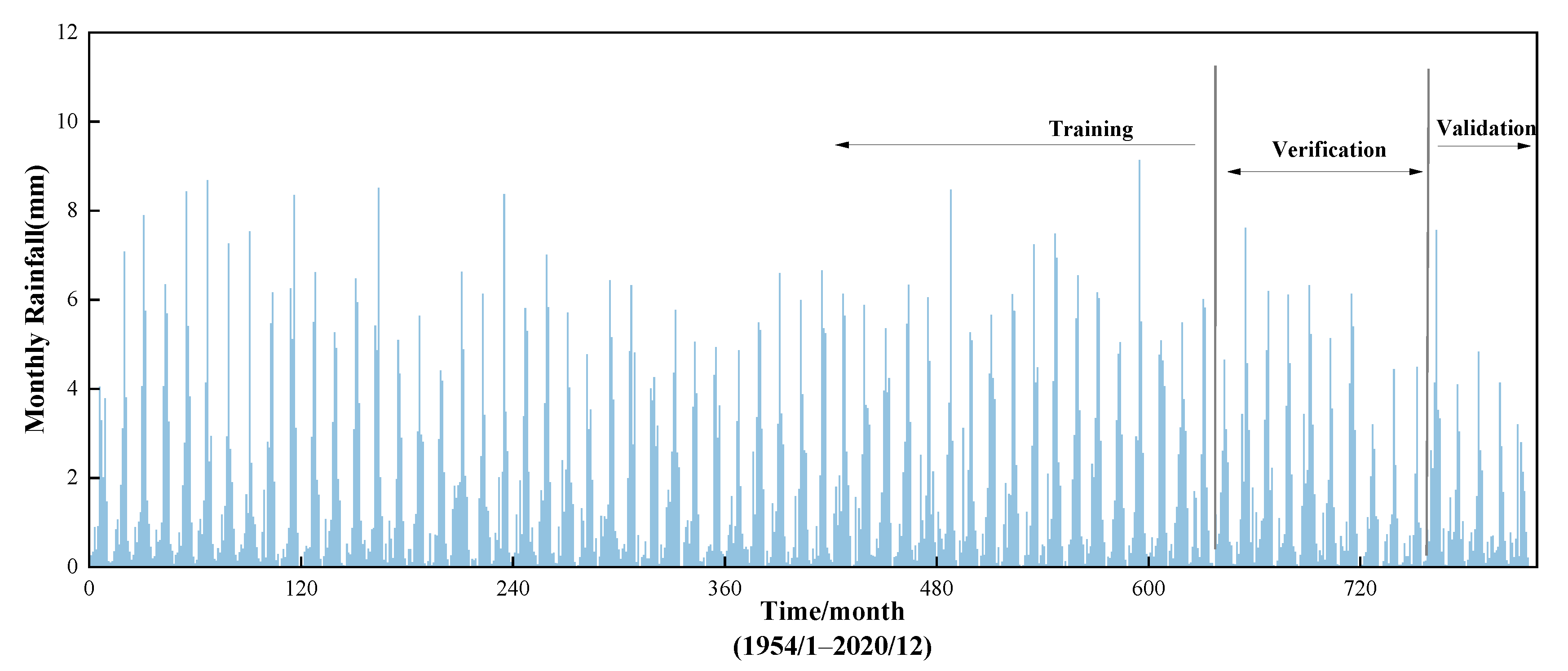
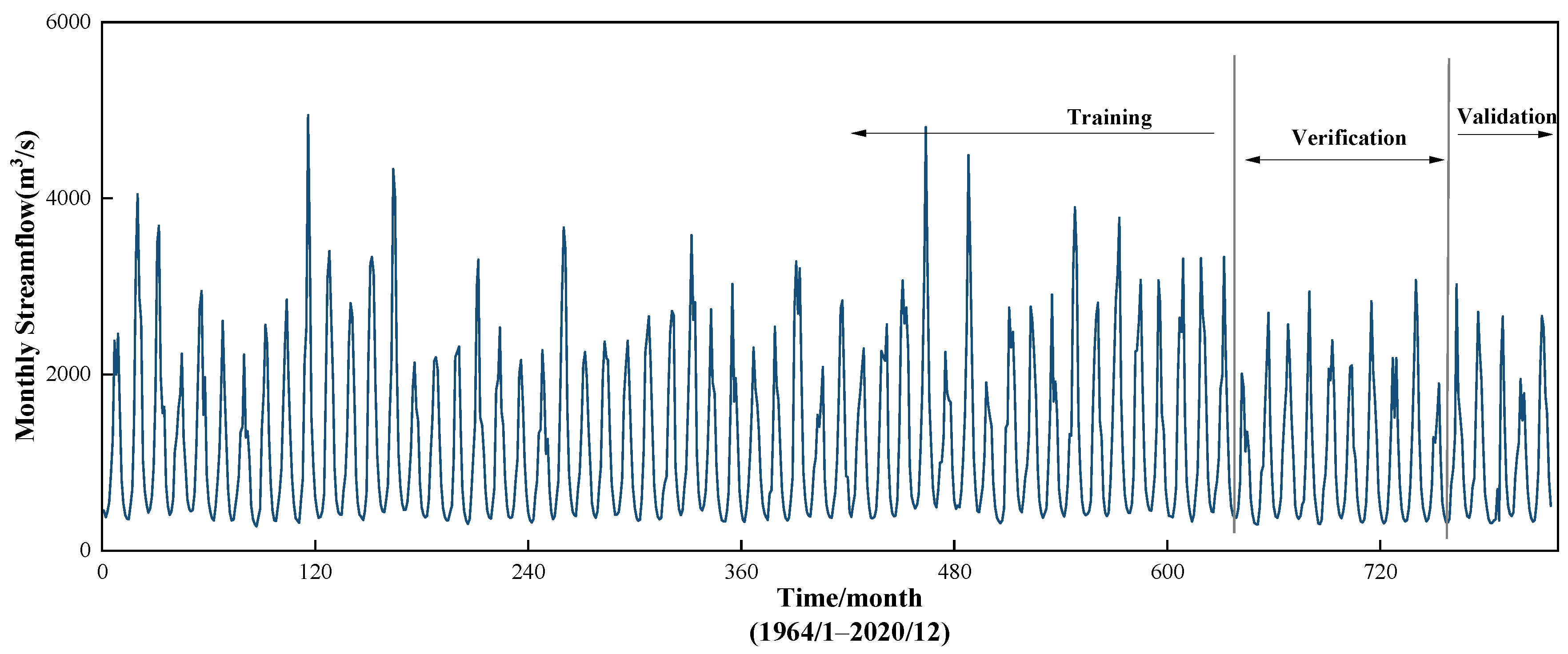
The dataset spanning from January 1954 to December 2005 is utilized for calibrating the parameters of the model described in Section 2.2, while the dataset from January 2006 to December 2015 is used to verify the model presented in Section 2.3 and determine the appropriate length of the reference period, and the monthly streamflow data from January 2016 to December 2020 are employed for validation. Figure 3 and Figure 4 depict the consecutive monthly rainfalls and runoffs from Xiaowan Hydrological Station; the streamflow process exhibits relative stability, indicating the reference value of the historical streamflow process for forecasting streamflow using the similarity-derived methods discussed in this study.
Selecting one similar year every ten annual streamflow sequences on average, the SDM set the parameter Y to five by considering approximately 50 years of historical monthly streamflow for model training. This work applies the models to the seasonal forecasting task of a power company in Yunnan, where the monthly streamflow into a reservoir at the beginning of a season must be forecasted for the upcoming season. Thus, the parameter, M ¯ , is three to represent the number of months to be predicted in a season. The SDM is configured to make runoff predictions for three months at a time, with these predictions rolling forward to cover the entire year’s monthly runoff. Therefore, the parameter m for prediction is set as 1, 4, 7, and 10 to indicate the forecast starting months of January, April, July, and October, allowing for the division of the annual monthly runoff predictions. The number of reference months will be tested as 3, 6, 9, and 12 in the verification dataset to assess its impact on the results in the next section, and then the parameters that demonstrate the best performance on the verification dataset will be selected and utilized for the subsequent validation section.
The prediction of monthly streamflow is performed using three methods for comparison purposes: the Mean method, which predicts streamflow for a given month as the average over historical months; the SDM proposed in this study; and the SVM implemented in MATLAB R2022a, where functions from the “Statistics and Machine Learning Toolbox”, including “fitcsvm” and “predict” are employed to utilize the SVM for runoff prediction.
The Gurobi 9.5.2 solver, run on a PC with an Intel(R) Core (TM) i3-8100 CPU at 3.60 GHz, is employed to solve the two quadratic problems proposed in this model.

3.2. Parameters in Calibration

Table 2 and Table 3 give the calibrated parameters λ t   and   β t with reference periods of 6 and 9 months, respectively, where the ‘m-6’ represents the 6th month proceeding the forecast-start month (m). The distribution of non-zero parameters in each month reveals that hydrological and meteorological data from the previous month of the forecast-start month play a crucial role in identifying similar years. The difference in magnitude between λ t   and   β t helps standardize the runoff and rainfall values, allowing for a consistent comparison between the two variables despite their different units.
Taking SDM6 as an example, during the process of using Gurobi for solving, the scale of the first QP problem includes 6636 constraints and 4450 variables, while the second QP problem comprises 28 constraints and 31 variables. When conducting the rolling predictions for a long sequence of monthly runoffs, the total solving time for both problems is 148.6 s.

3.3. Results in Verification

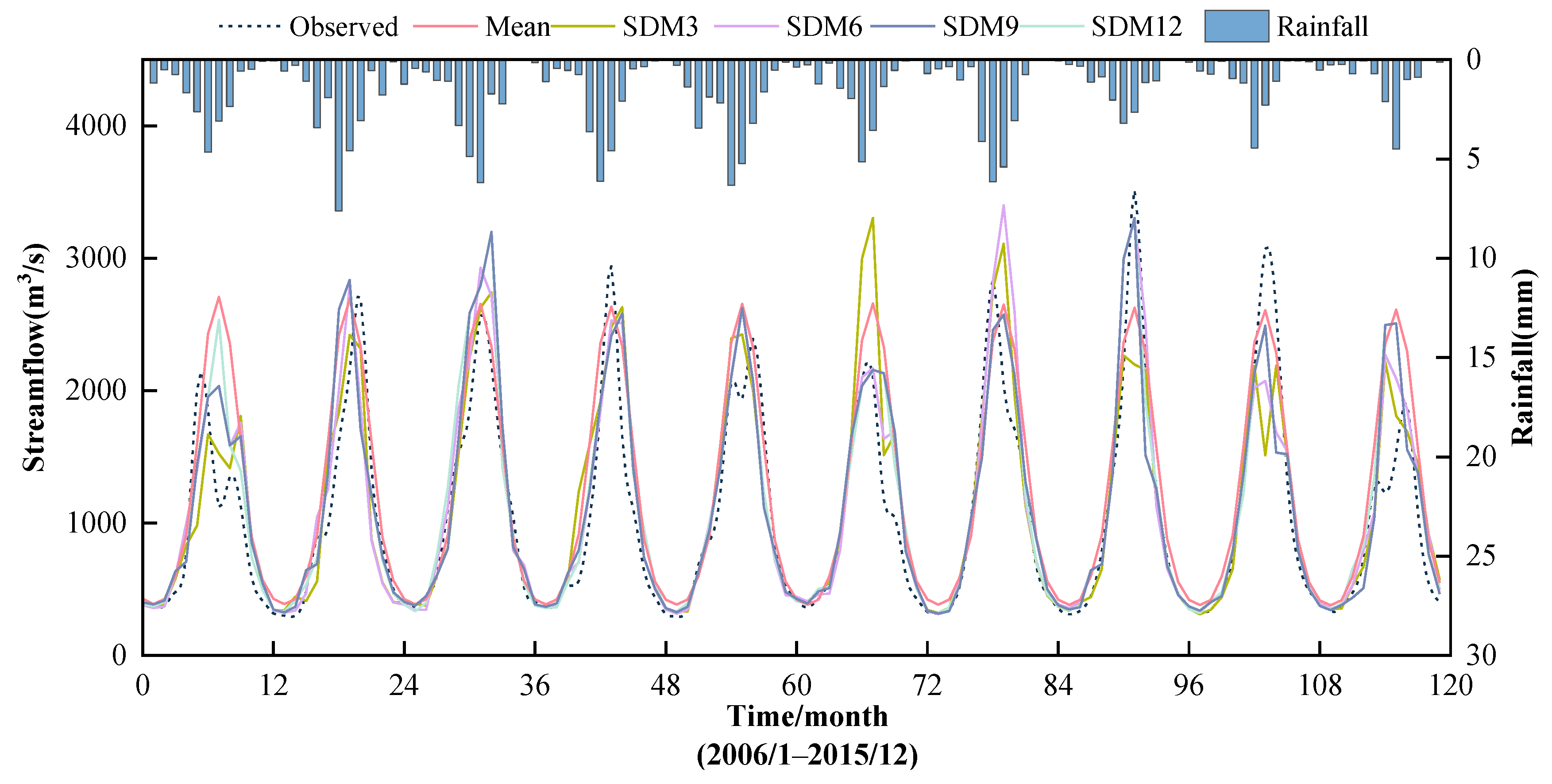
The predictive capability of the SDM is compared to that of the Mean method using data from 2006 to 2015, with the assessment of different reference periods (3, 6, 9, and 12 months) to determine the optimal choice. The SDMs, with different reference period lengths (SDM3, SDM6, SDM9, and SDM12), and the Mean method are evaluated for their predictive performance in predicting the monthly streamflow at Xiaowan, as shown in Table 4 and Figure 3.
Table 4 provides a comparison of the performance of the SDM under different reference periods. Indicating the accuracy of the predictions, the RMSE values for SDM3, SDM6, SDM9, and SDM12 are slightly lower than the Mean value of 374.47 m3/s, with SDM6 demonstrating the smallest RMSE value of 359.22 m3/s among the five methods. The Mean Absolute Percentage Error (MAPE) is employed to assess the accuracy of the model predictions in terms of relative errors, and the results indicate that the SDMs exhibit relative errors consistently more than 5% lower than the relative error of the Mean method, with SDM12 achieving the lowest of 18.3%. The Nash–Sutcliffe efficiency coefficient (NSE), a commonly used metric for evaluating the goodness of fit in hydrological model simulations, reveals that the SDMs outperform the Mean method, with SDM6 achieving the highest efficiency of 77.12%. The analysis of the results suggests that the SDMs, particularly SDM6, show better predictive ability than the monthly average values. Therefore, SDM6 was selected as the method with the best prediction accuracy and used for subsequent comparisons with other methods.
The predicted monthly streamflow and the corresponding rainfalls for the verification period from January 2006 to December 2015 are presented in Figure 5, demonstrating the good fit of the Mean and SDM methods to the observed values, with minor deviations observed in certain years.

3.4. Results in Validation

Based on the verification results in the previous section, this section compares the prediction performance of the SDM6, Mean, and SVM methods during the validation period. The evaluation results of the three methods in predicting the monthly streamflow series at Xiaowan are presented in Table 5 and Figure 6, Figure 7 and Figure 8. The SVM method was also evaluated using a reference period of 6 months and a forecast period of 3 months, consistent with SDM6.
Table 5 makes it evident that the Mean model has the lowest prediction accuracy compared to the other models, while the SVM shows improved prediction ability, with reductions of 26.25 m3/s in RMSE, 6.73% in MAPE, and an increase of 3.09% in NSE compared to the Mean model. However, SDM6 outperforms the SVM, with the RMSE and MAPE reduced by 53.65 m3/s and 0.24%, respectively, and the NSE improved by 5.53%. The results demonstrate that both the SVM and SDM6 outperform the Mean method in terms of predictive ability, with SDM6 showing the best performance overall based on the comprehensive evaluation of the RMSE, MAPE, and NSE.
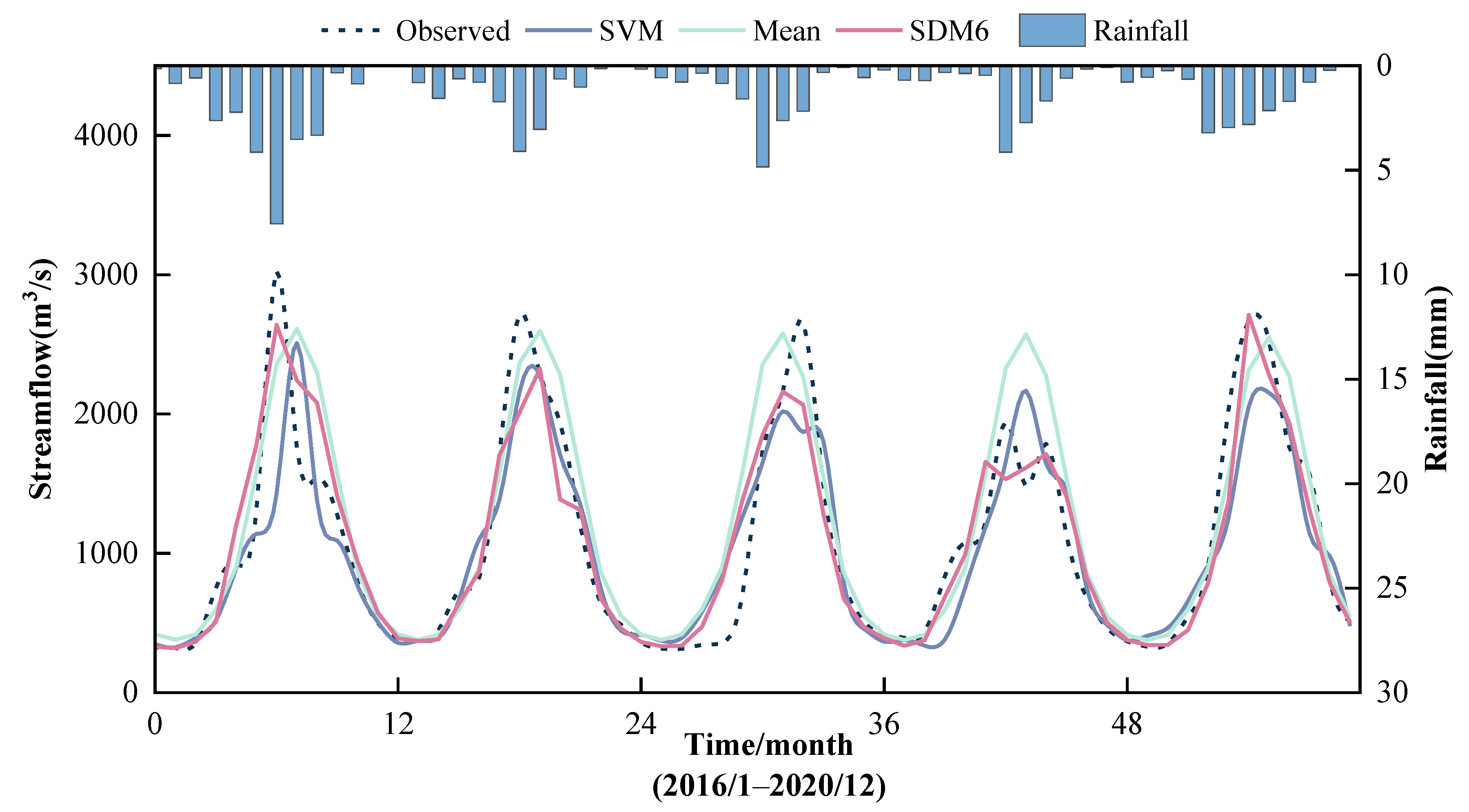
Figure 6 illustrates the prediction results during the validation period at Xiaowan Station using three models and includes the corresponding monthly rainfalls used in SDM6. In general, all the models exhibited a good fit during the dry season, while the Mean model performed the worst during the flood season, and SDM6 showed better performance than the Mean model, which is consistent with the findings in Table 5.
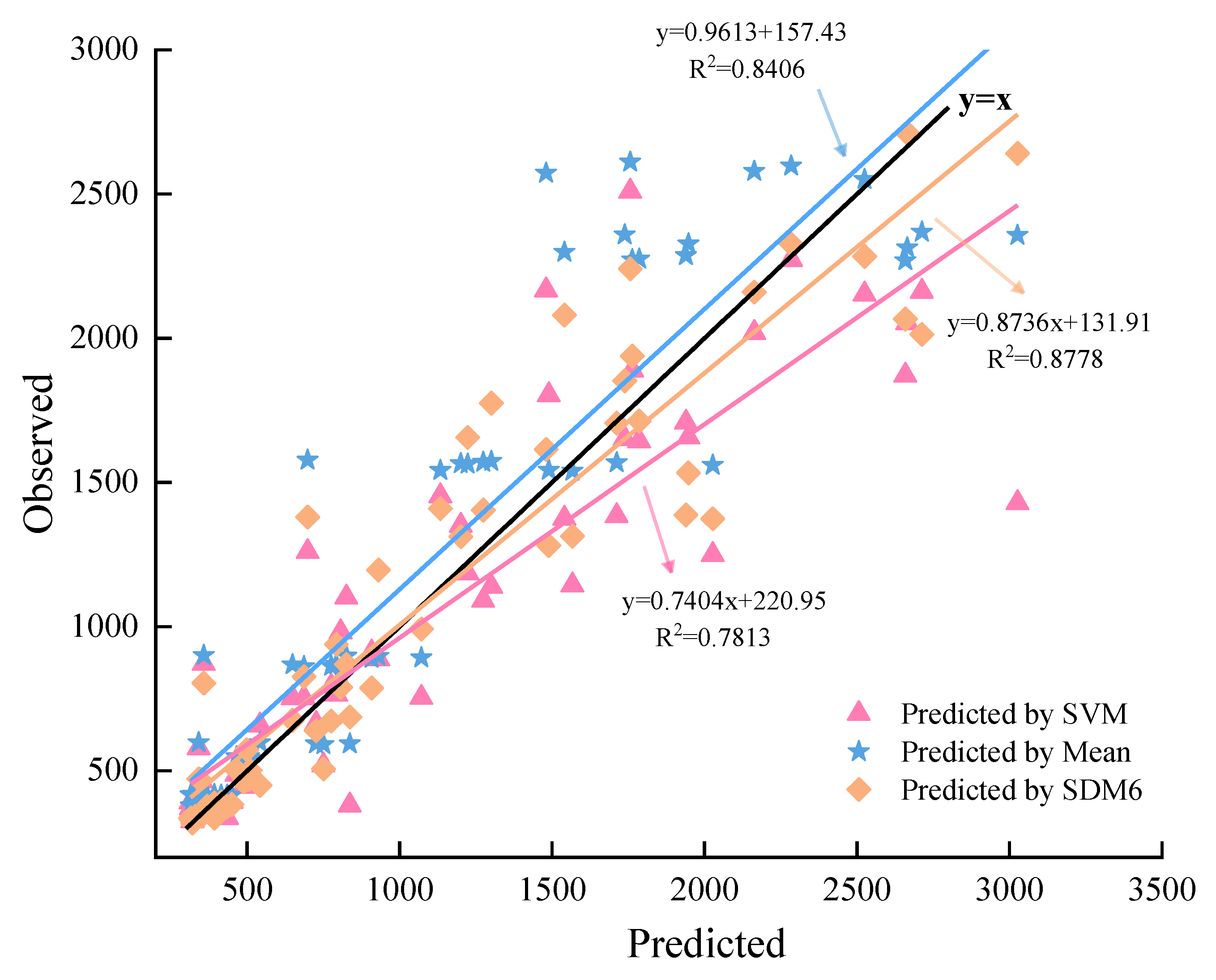
Figure 7 presents a scatter plot of the three prediction models at Xiaowan Station, revealing that the SVM has the poorest performance, with an R-squared value of 0.8406, while the linear trend of the Mean model closely aligns with the 45-degree line, with a slope of 0.9613, and the SDM exhibits the highest R-squared value of 0.8778, indicating that both SDM6 and the Mean model outperform the SVM in terms of accuracy measurement.
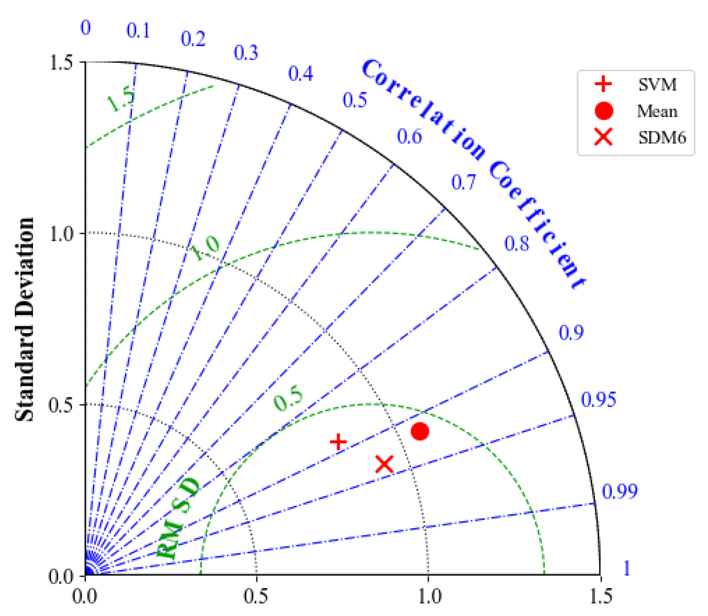
Figure 8 illustrates a Taylor diagram, showcasing the performance of streamflow prediction at Xiaowan Station during the validation period by the SVM, Mean model, and SDM6. The Taylor diagram displays the contours representing the Pearson correlation coefficient (blue), standard deviation (black), and Root Mean Square Deviation (RMSD in green), indicating the performance of streamflow prediction at Xiaowan Station by the SVM, Mean model, and SDM6 during the validation period. The results suggest that the SVM exhibits the lowest correlation coefficient, the highest standard deviation, and the largest difference in RMSD value from 1.0, indicating that it has the poorest performance compared to the Mean model and SDM6. SDM6 exhibits superior performance compared to the Mean model and SVM, as evidenced by its smallest RMSD value, largest correlation coefficient, and similar standard deviation levels close to 1.0, making it the best-performing model among the three.
To sum up, Figure 6, Figure 7 and Figure 8 present similar results, all indicating that the SDM prediction model demonstrates favorable fitting outcomes. Meanwhile, Table 5, which presents statistical metrics, indicates that the proposed SDM performs better in predicting the monthly streamflow at Xiaowan Station than the other two methods, with the highest NSE and smallest errors (RMSE and MAPE). The analysis demonstrates that the SDM can be effectively applied to monthly runoff forecasting.

4. Conclusions

This study presents an SDM that utilizes historical streamflow and rainfall sequences to identify similar patterns during a reference period preceding the forecast-start month and calculate predicted values for coming months. The model incorporates an analysis of patterns and underlying physical processes, making it a robust prediction method.
The SDM is compared with the SVM and Mean methods for streamflow prediction in case studies on the Lancang River, and the following results are obtained:
  • The assessment during a verification period on different reference periods (3, 6, 9, and 12) reveals that SDM6 with a reference period of six months demonstrates the best performance.
  • SDM6 during a validation period achieves 261.97 m3/s in RMSE, 16.01% in MAPE, and 87.74% in NSE, improving the Mean model by 79.9 m3/s in RMSE, 6.07% in MAPE, and 8.62% in NSE, and the SVM by 53.65 m3/s, 0.24%, and 5.53%, respectively.
The results above indicate that, despite utilizing data feature extraction and pattern recognition for runoff prediction, the Mean method effectively captures the general patterns in monthly runoff for this watershed. It performs well during low-flow months when water inflow is relatively stable but may struggle to predict the runoff during periods of unusually high or low water flow. Furthermore, the SVM relies on historical runoff patterns for prediction. However, its performance diminishes during years with non-stationary runoff processes, as it tends to predict relatively stable runoffs and may not effectively handle exceptional conditions. In contrast, the SDM utilizes historical runoff and rainfall data for pattern learning, enabling it to make predictions based on the watershed’s historical characteristics. It results in runoff predictions that align more closely with the actual conditions, better fitting the observed runoff processes.
There are some limitations of the SDM in applications, including the following:
(1)
The model requires relatively long historical runoff data, making it unsuitable for basins with short or discontinuous data records.
(2)
The model’s solving process requires multiple calls to the solver, leading to slower computation speed.
Still, there are numerous issues with this model that require further investigation. The future research directions for the model will include the following:
(1)
Future work can explore optimizing additional variables, including the number of similar years and forecast months, to further investigate the model’s performance.
(2)
Further investigation is warranted to understand the influence of historical rainfall on identifying the similar years used to derive the forecast streamflow.
(3)
The model and procedures may also be extended to encompass daily, weekly, and annual streamflow predictions.

Author Contributions

Conceptualization, J.W.; Methodology, Z.X.; Software, Z.X.; Resources, W.X.; Data curation, X.L.; Writing—original draft, Z.X.; Writing—review & editing, H.Z.; Visualization, M.C. All authors have read and agreed to the published version of the manuscript.

Funding

This research received no external funding.

Data Availability Statement

The data presented in this study are available on request from the corresponding author. The data are not publicly available due to data confidentiality.

Conflicts of Interest

The authors declare no conflict of interest.

References

  1. Napolitano, G.; Serinaldi, F.; See, L. Impact of EMD decomposition and random initialisation of weights in ANN hindcasting of daily stream flow series: An empirical examination. J. Hydrol. 2011, 406, 199–214. [Google Scholar] [CrossRef]
  2. Guo, J.; Zhou, J.; Qin, H.; Zou, Q.; Li, Q. Monthly streamflow forecasting based on improved support vector machine model. Expert Syst. Appl. 2011, 38, 13073–13081. [Google Scholar] [CrossRef]
  3. Wang, W.C.; Chau, K.W.; Cheng, C.T.; Qiu, L. A comparison of performance of several artificial intelligence methods for forecasting monthly discharge time series. J. Hydrol. 2009, 374, 294–306. [Google Scholar] [CrossRef]
  4. Huang, S.; Chang, J.; Huang, Q.; Chen, Y. Monthly streamflow prediction using modified EMD-based support vector machine. J. Hydrol. 2014, 511, 764–775. [Google Scholar] [CrossRef]
  5. Wang, X.; Engel, B.; Yuan, X.; Yuan, P. Variation Analysis of Streamflows from 1956 to 2016 Along the Yellow River, China. Water 2018, 10, 1231. [Google Scholar] [CrossRef]
  6. Zhu, S.; Zhou, J.; Ye, L.; Meng, C. Streamflow estimation by support vector machine coupled with different methods of time series decomposition in the upper reaches of Yangtze River, China. Environ. Earth Sci. 2016, 75, 531. [Google Scholar] [CrossRef]
  7. Huang, S.; Huang, Q.; Wang, Y.; Chen, Y. The study on the runoff change based on the heuristic segmentation algorithm and approximate entropy. Zhongshan Daxue Xuebao/Acta Sci. Natralium Univ. Sunyatseni 2014, 53, 154–160. [Google Scholar]
  8. Wang, W.C.; Xu, D.M.; Chau, K.W.; Chen, S. Improved annual rainfall-runoff forecasting using PSO-SVM model based on EEMD. J. Hydroinform. 2013, 15, 1377–1390. [Google Scholar] [CrossRef]
  9. Maxwell, R.M.; Chow, F.K.; Kollet, S.J. The groundwater-land-surface-atmosphere connection: Soil moisture effects on the atmospheric boundary layer in fully-coupled simulations. Adv. Water Resour. 2007, 30, 2447–2466. [Google Scholar] [CrossRef]
  10. Yetemen, O.; Istanbulluoglu, E.; Flores-Cervantes, J.H.; Vivoni, E.R.; Bras, R.L. Ecohydrologic role of solar radiation on landscape evolution. Water Resour. Res. 2015, 51, 1127–1157. [Google Scholar] [CrossRef]
  11. Sulis, M.; Paniconi, C.; Marrocu, M.; Huard, D.; Chaumont, D. Hydrologic response to multimodel climate output using a physically based model of groundwater/surface water interactions. Water Resour. Res. 2012, 48, W12510. [Google Scholar] [CrossRef]
  12. Ebel, B.A.; Mirus, B.B. Disturbance hydrology: Challenges and opportunities. Hydrol. Process. 2014, 28, 5140–5148. [Google Scholar] [CrossRef]
  13. Van Roosmalen, L.; Sonnenborg, T.O.; Jensen, K.H. Impact of climate and land use change on the hydrology of a large-scale agricultural catchment. Water Resour. Res. 2009, 45, W00A15. [Google Scholar] [CrossRef]
  14. Pierini, N.A.; Vivoni, E.R.; Robles-Morua, A.; Scott, R.L.; Nearing, M.A. Using observations and a distributed hydrologic model to explore runoff thresholds linked with mesquite encroachment in the Sonoran Desert. Water Resour. Res. 2014, 50, 8191–8215. [Google Scholar] [CrossRef]
  15. Partington, D.; Brunner, P.; Simmons, C.T.; Werner, A.D.; Therrien, R.; Maier, H.R.; Dandy, G.C. Evaluation of outputs from automated baseflow separation methods against simulated baseflow from a physically based, surface water-groundwater flow model. J. Hydrol. 2012, 458–459, 28–39. [Google Scholar] [CrossRef]
  16. Bathurst, J.C.; O’Connell, P.E. Future of distributed modelling: The Systeme Hydrologique Europeen. Hydrol. Process. 1992, 6, 265–277. [Google Scholar] [CrossRef]
  17. Kumar, S.; Tiwari, M.K.; Chatterjee, C.; Mishra, A. Reservoir Inflow Forecasting Using Ensemble Models Based on Neural Networks, Wavelet Analysis and Bootstrap Method. Water Resour. Manag. 2015, 29, 4863–4883. [Google Scholar] [CrossRef]
  18. Wen, X.; Feng, Q.; Deo, R.C.; Wu, M.; Yin, Z.; Yang, L.; Singh, V.P. Two-phase extreme learning machines integrated with the complete ensemble empirical mode decomposition with adaptive noise algorithm for multi-scale runoff prediction problems. J. Hydrol. 2019, 570, 167–184. [Google Scholar] [CrossRef]
  19. Raman, H.; Sunilkumar, N. Multivariate modelling of water resources time series using artificial neural networks. Hydrol. Sci. J. 1995, 40, 145–163. [Google Scholar] [CrossRef]
  20. Afan, H.A.; El-Shafie, A.; Yaseen, Z.M.; Hameed, M.M.; Wan Mohtar, W.H.M.; Hussain, A. ANN Based Sediment Prediction Model Utilizing Different Input Scenarios. Water Resour. Manag. 2015, 29, 1231–1245. [Google Scholar] [CrossRef]
  21. Moreido, V.; Gartsman, B.; Solomatine, D.P.; Suchilina, Z. How Well Can Machine Learning Models Perform without Hydrologists? Application of Rational Feature Selection to Improve Hydrological Forecasting. Water 2021, 13, 1696. [Google Scholar] [CrossRef]
  22. Yaseen, Z.M.; El-shafie, A.; Jaafar, O.; Afan, H.A.; Sayl, K.N. Artificial intelligence based models for stream-flow forecasting: 2000–2015. J. Hydrol. 2015, 530, 829–844. [Google Scholar] [CrossRef]
  23. Mosavi, A.; Ozturk, P.; Chau, K.-W. Flood Prediction Using Machine Learning Models: Literature Review. Water 2018, 10, 1536. [Google Scholar] [CrossRef]
  24. Chang, F.J.; Chen, Y.C. A counterpropagation fuzzy-neural network modeling approach to real time streamflow prediction. J. Hydrol. 2001, 245, 153–164. [Google Scholar] [CrossRef]
  25. Ni, Q.; Wang, L.; Ye, R.; Yang, F.; Sivakumar, M. Evolutionary modeling for streamflow forecasting with minimal datasets: A case study in the West Malian River, China. Environ. Eng. Sci. 2010, 27, 377–385. [Google Scholar] [CrossRef]
  26. Zhan, X.; Qin, H.; Liu, Y.; Yao, L.; Xie, W.; Liu, G.; Zhou, J. Variational Bayesian Neural Network for Ensemble Flood Forecasting. Water 2020, 12, 2740. [Google Scholar] [CrossRef]
  27. Hu, C.; Wu, Q.; Li, H.; Jian, S.; Li, N.; Lou, Z. Deep Learning with a Long Short-Term Memory Networks Approach for Rainfall-Runoff Simulation. Water 2018, 10, 1543. [Google Scholar] [CrossRef]
  28. Zhao, X.; Chen, X.; Xu, Y.; Xi, D.; Zhang, Y.; Zheng, X. An EMD-Based Chaotic Least Squares Support Vector Machine Hybrid Model for Annual Runoff Forecasting. Water 2017, 9, 153. [Google Scholar] [CrossRef]
  29. Coulibaly, P.; Baldwin, C.K. Nonstationary hydrological time series forecasting using nonlinear dynamic methods. J. Hydrol. 2005, 307, 164–174. [Google Scholar] [CrossRef]
  30. Chu, H.; Wei, J.; Wu, W.; Jiang, Y.; Chu, Q.; Meng, X. A classification-based deep belief networks model framework for daily streamflow forecasting. J. Hydrol. 2021, 595, 125967. [Google Scholar] [CrossRef]
  31. Danandeh Mehr, A.; Kahya, E. A Pareto-optimal moving average multigene genetic programming model for daily streamflow prediction. J. Hydrol. 2017, 549, 603–615. [Google Scholar] [CrossRef]
  32. Maass, A.; Hufschmidt, M.M.; Dorfman, R.; Thomas Jr, H.A.; Marglin, S.A.; Fair, G.M. 12. Mathematical Synthesis of Streamflow Sequences for the Analysis of River Basins by Simulation. In Design of Water-Resource Systems: New Techniques for Relating Economic Objectives, Engineering Analysis, and Governmental Planning; Harvard University Press: Cambridge, MA, USA, 1962. [Google Scholar]
  33. Cortes, C.; Vapnik, V. Support-Vector Networks. Mach. Learn. 1995, 20, 273–297. [Google Scholar] [CrossRef]
  34. Rojo, J.D.; Carvajal, L.F.; Velasquez, J.D. Streamflow Prediction using a Forecast Combining System. IEEE Lat. Am. Trans. 2015, 13, 1035–1040. [Google Scholar] [CrossRef]
  35. Fan, H.; He, D.M.; Wang, H.L. Environmental consequences of damming the mainstream Lancang-Mekong River: A review. Earth Sci. Rev. 2015, 146, 77–91. [Google Scholar] [CrossRef]
  36. Liu, J.G.; Chen, D.L.; Mao, G.Q.; Irannezhad, M.; Pokhrel, Y. Past and Future Changes in Climate and Water Resources in the Lancang-Mekong River Basin: Current Understanding and Future Research Directions. Engineering 2022, 13, 144–152. [Google Scholar] [CrossRef]
Figure 1. Pre-processing the monthly streamflow and rainfall over multiple years.
Water 15 03270 g001
Figure 2. The Lancang River Basin.
Water 15 03270 g002
Figure 3. The observed monthly rainfalls at Xiaowan Station from 1954/1 to 2020/12.
Water 15 03270 g003
Figure 4. The observed monthly runoffs at Xiaowan Station from 1954/1 to 2020/12.
Water 15 03270 g004
Figure 5. Comparison of monthly streamflow forecasted during the verification period.
Water 15 03270 g005
Figure 6. Comparison of forecasted monthly streamflow in validation among three methods.
Water 15 03270 g006
Figure 7. Scatter plot of predictions by three models at Xiaowan Station.
Water 15 03270 g007
Figure 8. Taylor diagram of prediction by three models at Xiaowan Station.
Water 15 03270 g008
Table 1. The statistics of monthly streamflow at Xiaowan Hydrological Station.
StationPeriodMax (m3/s)Min (m3/s)Mean (m3/s)CvCs
Xiaowan1954–20204948.0275.01201.550.731.15
Table 2. The calibration results of parameters with a reference period of six.
Ref (t) λ t β t
JanAprJulOctJanAprJulOct
m-600000.73296.659540
m-51.10 × 10−52.90 × 10−37.60 × 10−100.4000
m-41.60 × 10−5007.50 × 10−41.4000
m-38.80 × 10−5001.20 × 10−20000
m-20004.50 × 10−400026.8
m-14.10 × 10−33.30 × 10−17.60 × 10−39.40 × 10−451.1772.11401.997.4
Table 3. The calibration results of parameters with a reference period of nine.
Ref (t) λ t β t
JanAprJulOctJanAprJulOct
m-91.80 × 10−30000001491.6
m-81.00 × 10−3009.90 × 10−217.2001505.1
m-703.60 × 10−500034.560,073.3559
m-600003.6337.911,402.20
m-58.10 × 10−54.10 × 10−19.40 × 10−101.7000
m-41.60 × 10−4002.70 × 10−311.7000
m-35.50 × 10−4003.20 × 10−30000
m-20001.30 × 10−300031.5
m-12.40 × 10−23.10 × 10−29.90 × 10−33.00 × 10−3156.7691804.5330.9
Table 4. Performances of SDMs and Mean method for verification at Xiaowan Station.
IndicatorsMEANSDM3SDM6SDM9SDM12
RMSE (m3/s)374.47371.31359.22370.57373.14
MAPE (%)23.8218.5918.4618.3918.3
NSE (%)75.1375.5577.1275.6575.31
Table 5. The performance in validation prediction at Xiaowan Station.
IndicatorsMeanSVMSDM6
RMSE (m3/s)341.87315.62261.97
MAPE (%)22.9816.2516.01
NSE (%)79.1282.2187.74
Disclaimer/Publisher’s Note: The statements, opinions and data contained in all publications are solely those of the individual author(s) and contributor(s) and not of MDPI and/or the editor(s). MDPI and/or the editor(s) disclaim responsibility for any injury to people or property resulting from any ideas, methods, instructions or products referred to in the content.