Abstract
Flash floods are increasingly frequent worldwide. Recent flooding in eastern Ethiopia resulted in casualties, destruction of property and interruptions of service. National flash flood forecasts made today primarily consider precipitation, putting less emphasis on surface processes. Enhancing accurate flash flood forecasts by accounting for surface processes and hydrological models together with a deeper understanding of heavy precipitation mechanisms is of paramount importance. To this end, an uncoupled WRF-Hydro model was calibrated for eastern Ethiopia to simulate extreme floods. Sensitivity analysis for August 2006 showed that infiltration runoff, hydraulic soil conductivity and saturated volumetric soil moisture with parameter values of 0.1, 1.5 and 1.0 produced realistic streamflow distribution. Extreme floods in March 2005 and April 2007 were further studied. The results showed that WRF-Hydro replicates temporal and spatial patterns well. Analysis using observational/reanalysis data revealed associated physical processes. Precipitation during these events exceeded long-term climatology and spanned wider areas in eastern Ethiopia. These heavy precipitation events are associated with strong upper-level westerly jet streams and rainfall-conducive circulation anomalies at lower levels. Positive outcomes from WRF-Hydro suggest operational implementation for flood monitoring and early warning systems in forecasting centers.
1. Introduction
Worldwide, floods are responsible for 40–50% of all disasters and disaster-related fatalities [1,2]. The frequency and severity of floods in Africa have grown over the past several decades [3], which has had a substantial impact on the people and infrastructure of the globe [4,5,6,7]. For instance, in September 2009, 16 nations in West Africa were affected by torrential rain and flooding, which left 600,000 people in a difficult situation. This incident occurred shortly after the 2007 floods, which caused more than a million people to be displaced and claimed more than 500 lives in nations including Uganda, Ethiopia, Sudan, Burkina Faso, Togo, Mali and Niger, as well as the 2008 floods in Mozambique [8]. Floods in Africa frequently result in extensive damage to crops and loss of infrastructure, including roads, bridges and buildings, which causes food shortages and famine. In addition, flooding in Africa worsens the spread of water-borne illnesses like cholera and typhoid, which has an even greater negative effect on community health and well-being [9].
Several episodes of extreme precipitation or lack of it have led to high-impact floods and droughts over East Africa. Furthermore, the frequency of the fatality caused by intense precipitation events and flash floods is increasing with time [10]. For instance, in the city of Dire Dawa, flash floods frequently resulted from significant rainfall events, which had disastrous effects on both infrastructure and occupants [11,12,13]. Spring is the season when the majority of heavy precipitation events occur over Dire Dawa. The 2005 flood event that caused the death of more than 35 people and an estimated amount of ETB 10 million damages to property due to the heavy precipitation and flooding that occurred in the spring season [14]. It is important to note that floods can also occur during summer season, where it is the main rainy season for most of the western and central highland areas. For instance, in 2006, more than 200 people were dead and 3000 displaced by flash floods that occurred in August [15]. In addition, climate models broadly project an increase in the frequency of heavy precipitation over several parts of the world in the future warmer world due to an increase in anthropogenic greenhouse gas emissions [16,17,18,19,20]. However, projections from global models are subject to uncertainty at regional and local scales due to their coarse resolution. This implies that there is a need for a realistic simulation and a thorough understanding of the flood characteristics in the current climate in order to plan for a proper adaptation strategy.
Operational centers in East Africa provide flood early warnings entirely based on precipitation outlooks with little emphasis on surface processes that play a key role in modulating flood events. Conceptual models employing lumped parameters to depict the collective behavior of an entire catchment as a unified entity offer a valuable tool for flood forecasting by capturing the dynamics of surface processes [21,22]. Numerous studies (for example, [23,24,25,26,27]) have demonstrated that high-resolution land-surface-based hydrological models are able to simulate the pick, timing and spatial distribution of flood events reasonably. WRF-Hydro stands out as a commonly employed hydrological model, incorporating a range of physics-based and conceptual methodologies. This enhances the accuracy of simulations for land surface hydrology, energy distribution and flows, often achieved at a relatively fine spatial resolution, generally around 1 km or even finer. For instance, recent research by [24,28] indicated the model capability for streamflow simulation after calibrating the uncoupled WRF-Hydro model in two basins (the Gila River and Babocomari River basins) in southern Arizona. It is important to emphasize that, in the uncoupled version, the hydrological model simulates the surface/hydrological processes using atmospheric forcing obtained from external sources lacking two-way interaction. However, in the coupled version of WRF-Hydro, both the hydrological model (Hydro) and the WRF model are integrated. Consequently, hydrological and atmospheric processes are simulated simultaneously and mutually influence each other. Similar research by [29] demonstrated that the WRF-Hydro modeling framework accurately reproduces flash flood behavior and can fairly predict runoff observations throughout six watersheds on New Caledonia’s tropical island (SW Pacific). Furthermore, ref. [30] employed the WRF-Hydro model over the Tana River basin in East Africa to quantify the terrestrial water balance. Numerous previous studies (e.g., [31,32,33]) have also demonstrated that the WRF-Hydro model can actually replicate observed streamflow and discharge patterns across different river basins. Some have even implemented the WRF-Hydro model in their operational flood forecasting (e.g., [34] for the US and [35] for Israel). However, less emphasis is placed on the use of land-surface-based hydrological models for flood prediction over East Africa. Therefore, one of the objectives of this paper is to configure, simulate, calibrate and verify if uncoupled WRF-Hydro can be used to predict flood events. The uncoupled WRF-Hydro model is chosen because it allows us to focus only on the hydrological components. In particular, when the model is driven by reanalysis/observation, it will remove any uncertainty coming from atmospheric processes. Moreover, the uncoupled WRF-Hydro model uses fewer computational resources than the coupled WRF-Hydro model, which enables us to run more simulations for the same computing resources.
Detailed investigation and understanding of meteorological and hydrological processes associated with these extreme precipitations that led to past flooding events can be of value to improve early warning systems. Past studies [36,37,38,39,40,41] suggested the main large-scale atmospheric factors causing heavy precipitation at sub-seasonal and seasonal time scale in the region are linked to the intensity of the high-pressure system over the Arabian sea, the southward shift of subtropical westerly jet streams, North Atlantic Oscillation [42] and Madden–Julian Oscillation (MJO) [39]. Nonetheless, the corpus of scientific research on heavy rainfall events that cause floods in East Africa, particularly at short time scales in metropolitan areas, is still rather small. This paper, therefore, aims to investigate the role of large-scale atmospheric and oceanic features associated with recent high-impact flooding events that have occurred in Dire Dawa. We will investigate the details of the synoptic evolution and infer the intensity of these events from climatological perspectives.
The paper is set up as follows. The data, method and model description are provided in Section 2. Section 3 will discuss the calibration of the uncopuled WRF-Hydro model. The main results of WRF-Hydro case studies together with meteorological analysis are discussed in Section 3. Finally, a summary and thoughts on future work are provided in Section 4.
2. Domain, Data and Model Description
2.1. Study Area
The eastern region of Ethiopia contains distinctive topographical features that can control regional hydrological phenomena. Figure 1a,b show several topographic features of interest, as well as providing the location of Dire Dawa city and its environs. Notable among the topographic features are the mountain ranges surrounding the city. As discussed in [43], topographic characteristics have a significant impact on the development and organization of the hydrology linked to heavy precipitation.
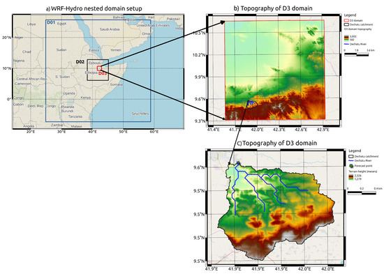
Figure 1.
(a) Map of East Africa showing the location of model domains at 25, 5 and 1 km horizontal resolution (D1, D2 and D3, respectively). D1 is defined by 150 × 150 grid points and extends 0 to 17 N and 30 to 55 E); D2 and D3 are defined with 150 × 150 grid points; (b) topography of D3 domain; (c) river channels in D3 domain with the focus of Dechatu River catchment and forecast point.
This study is being carried out in the Ethiopian city of Dire Dawa, which frequently experiences flooding hazards. Here, we are interested to investigate the Dechatu River catchment, which is believed to be the cause of severe flash flooding in Dire Dawa city [11]. The Dechatu River pointed in the N-NW direction as indicated in Figure 1c and it is originated in the northern escarpment of Harerge plateau.
Figure 2 indicates the maps of land category and soil type in 1 km pixels of Dechatu River catchment derived from Moderate Resolution Imaging Spectroradiometer (MODIS) dataset. Grasslands and Open Shurblands are dominant land classes in this catchment, as indicated in Figure 2a. The whole Dechatu River catchment is indicated to have clay loam soil type, as shown in Figure 2b. Clay loam is a soil mixture that contains more clay than other types of rock or minerals. One of clay’s most significant qualities is the size of its particles, which is quite small. As a result, loams that contain a predominance of clay tend to be heavy because they are so dense.
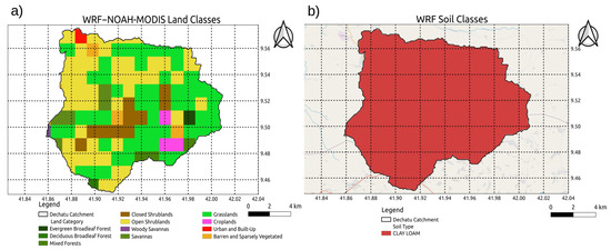
Figure 2.
Maps of dominant (a) land category and (b) soil type of Dachatu River catchment.
In gridded routing, the WRF-Hydro model’s FLOWDIRECTION variable clearly describes flow directions along the channel network. This factor determines where water enters channels both from the surface of the ground and inside the channel. Figure 3a indicates the WRF-Hydro default flow direction grid along the Dechatu River catchment. We used the void filled digital elevation data of HydroSHEDS core products to validate the flow direction obtained from WRF-Hydro model. The flow direction acquired from HydroSHEDS data along Dechatu River catchment is indicated in Figure 3b. The flow direction in the figure is similar to that of Figure 3a, which means the flow direction attained from the WRF-Hydro model reasonably represents the flow direction along the Dechatu River catchment.
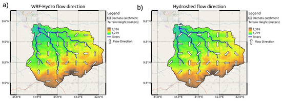
Figure 3.
(a) Dechatu River watershed along with WRF-Hydro default flow direction; (b) Dechatu River watershed along with hydroshed flow direction.
2.2. Observational and Gridded Datasets
We used several atmospheric variables (wind, radiation, temperature, humidity, surface pressure and precipitation) from ERA5 [44] reanalysis data and verification rainfall data from merged satellite–gauge precipitation observations [45,46]. The European Centre for Medium-range Weather Forecasts’s (ECMWF) ERA5 is produced by assimilating observations and the Integrated Forecast System at a resolution of 0.25 and available from 1979 until near real time [44].
The observed flow depth of Dechatu River catchment is provided with daily resolution from Ethiopian Ministry of Water and Energy. To conduct the comparison, we consider the daily maximum of the flow depth measured at the outlet of the Dechatu River obtained from the uncoupled WRF-Hydro model for the specified period.
Two daily observational precipitation datasets were used. These are the Global Precipitation Climatology Centre [46], which is available at 1 degree resolution for the 1988–2005 period, and precipitation dataset from the climate hazards infrared precipitation station [45]. CHIRPS is built by combining station data with infrared satellite estimated precipitation, making it appealing for regions with a scarcity of data, like Africa. CHIRPS data are available from 1981 onwards. Both datasets are interpolated on to a common 0.25 grid resolution.
The 250 m, 1 km and 5 km spatial resolution Digital Elevation Model (DEM) data were generated by [47]. These DEMs were obtained from EarthEnv: Global, Remote Sensing Supported Environmental Layers for Assessing Status and Trends in Biodiversity, Ecosystems, and Climate http://www.earthenv.org/topography, accessed in 1 March 2023. The former GMTED [48] served as the main dataset due to its full global extent and having the highest resolution (250 m). In areas where the scopes of the two datasets overlap (56 S–60 N latitude), the later SRTM [49], created by the Consultative Group for International Agriculture Research-Consortium (CGIAR), was utilized for comparing and validating the GMTED-derived variables and evaluating the impact of spatial scale acquisition.
2.3. Model Description
The uncoupled hydrological modeling system used in this study consists of the two models, the non-hydrostatic Weather Research and Forecasting (WRF) model [50], which is used to define the domains and initial conditions. The other model is WRF-Hydro, which is responsible for handling the hydrological process. A brief overview of these two models is presented in Section 2.3.1 and Section 2.3.2.
2.3.1. WRF Model
WRF model version 4.3 [50] is employed in this paper. The model consists of three nested domains as indicated in Figure 1a. The parent domain, D1, has 25 km horizontal resolution, and it is defined with 150 × 150 grid points. The D1 domain is covering Sudan, South Sudan, Uganda, Kenya, Ethiopia, Eritrea, Somalia, Yemen and parts of Indian Ocean (0 to 17 N and 30 to 55 E), thus capturing a broad range of weather systems. D2 and D3 are defined with 150 × 150 grid points with horizontal resolution of 5 km and 1 km, respectively.
The D3 domain and the associated stream channels are indicated in Figure 1c. The D3 domain further decomposed to finer horizontal resolution of 250 m to handle the routing process. The grid size selection corresponds to [51], which indicates that a grid resolution of 250 m × 250 m is an optimal choice for effectively and accurately forecasting flash floods using the WRF-Hydro routing model, considering both performance and computational needs. The simulation setup related to the routing processes will be explained further in Section 2.3.2.
The simulations are initialized on 1 January 2006. NCEP (National Centers for Environmental Prediction) FNL (Final) operational global analysis data [52] provide the initial and lateral boundary conditions for the simulations. Further details of the WRF configurations and physics schemes and parameter settings used in this study are indicated in Table 1.

Table 1.
Configuration details of the atmospheric model, WRF.
2.3.2. WRF-Hydro Model
The WRF-Hydro model is a distributed, community-based system that integrates the WRF atmospheric model with simulation modules for lateral water flow and aquifer activities [53]. Both uncoupled (independently or offline) and coupled (in combination with other Earth System modeling systems, such as an atmospheric model) applications of the model are possible. This study used the uncoupled WRF-Hydro model to investigate flooding events in Dire Dawa.
The uncoupled mode functions like any other land surface hydrological modeling system and behaves as a standalone land surface model (in our instance, Noah-MP LSM). It needs gridded meteorological forcing data that have been prepared and provided externally. The flowchart that indicates all the processes required to conduct WRF-Hydro uncoupled simulation is indicated in Figure 4. Major land surface processes, such as surface energy balance, runoff production and infiltration, aquifer recharge and snow melt and accumulation, are handled by Noah-MP LSM. Runoff generation and infiltration processes are discussed further in Section 2.4 since we noticed the parameters related to this process are critical for model calibration for our study area. Table 2 lists the physics options used for the application of Noah-MP.
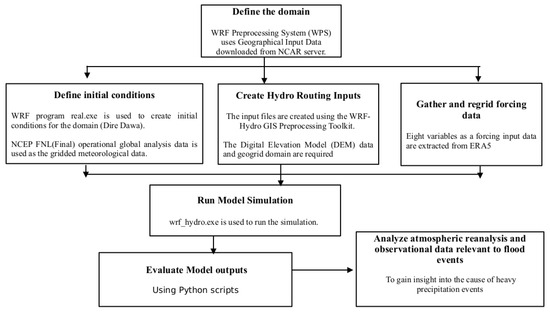
Figure 4.
Flow chart indicates all the processes required to conduct WRF-Hydro uncoupled simulation, starting from defining the domain to the evaluation of model outputs.
Table 2.
Selected physics options of Noah-MP LSM. The ID numbers are used to identify the values that can be entered into the model input file.
2.4. Runoff Generation and Infiltration
Four soil layers that extend up to 2 m are used: 0.1 m, 0.3 m, 0.6 m and 1 m thickness for 1st, 2nd, 3rd and 4th layers, respectively. Depending on the moisture content of the soil and the amount of precipitation, runoff can be created or water can infiltrate through the soil layers and percolate to an underlying unconfined aquifer. In this work, runoff production was simulated using the infiltration-excess-based surface runoff schemes [54,55].
Surface runoff [mm], R, equals the difference between precipitation [mm], P, and maximum infiltration, (). Infiltration maximum [mm] is computed as an increasing function of the liquid soil moisture deficit of the soil column :
where is time step of the model, depending on soil texture, REFDK is a reference saturated hydraulic conductivity of silty clay loam, assumed spatially constant and equal to m/s, DKSAT [ms] is the saturated hydraulic soil conductivity and REFKDT [unitless] is the surface infiltration coefficient. The values of REFDK and REFKDT are constant on the whole domain.
2.5. Model Performance Evaluation Metrics
Some quantitative data are needed to measure model performance in order to calibrate, validate and compare the models. The flow depth data collected at the Dechatu River watershed’s outlet is used in this study to evaluate the model’s performance. We used statistical indices such as the Nash–Sutcliffe efficiency (NSE), root mean square error (RMSE) and RMSE observations standard deviation ratio (RSR) to quantify model performance.
The range of the Nash–Sutcliffe efficiency coefficient (NSE) is −∞ to 1. When NSE = 1 (Equation (A3)), it denotes a perfect agreement between the observed and anticipated values. In general, values between and are regarded as acceptable performance levels [56], but values below show that the mean observed value is higher than the simulated value, which denotes unacceptable performance. When the RMSE (Equation (A4)) equals 0, the observed and predicted values match perfectly, and, as the RMSE increases, the quality of the simulation deteriorates. The ratio of the RMSE and standard deviation of measured data are used to determine the RMSE observations standard deviation ratio (RSR) as shown in Equation (A5). RSR ranges from a high positive value to the ideal value of zero. The performance of the model simulation increases with decreasing RMSE and RSR.
3. Results and Discussion
3.1. Calibration of the Uncopuled WRF-Hydro Model
Many parameters in the uncoupled WRF-Hydro model have significant uncertainty that can potentially alter the calculation of the runoff, as indicated in Equations (1), (A1) and (A2).
Further, 2-month spin-up simulations were performed prior to the calibration to ensure the numerical stability of the model outputs. We used default configuration with the original surface and subsurface runoff option (). The default configuration parameters have values of , and for REFKDT, DKSAT and SMCMAX, respectively. Meteorological forcing data were extracted from the ERA5 dataset. The standalone WRF-Hydro model requires eight meteorological input variables, which include hourly incoming shortwave radiation (SWDOWN Wm), incoming longwave radiation (LWDOWN Wm), specific humidity (Q2D kg/kg), air temperature at 2 m above the surface (T2D K), surface pressure (PSFC Pa), near-surface wind in the u-component (U2D ms), near-surface wind in the v-component (V2D ms) and precipitation rate (RAINRATE mms). After the spin-up, “restart” NetCDF files were created and used to start the simulations on 1 August 2006 with the proper values for the state variables. The simulated stream discharge does not respond to the precipitation rate during the model spin-up period (1 June–31 July 2006), shown in Figure A1, and it continuously decreases throughout the simulation period. This means the model is not doing a good job in representing the stream discharge.
To improve the results obtained during the model spin-up, calibration is conducted on the parameters that control surface runoff. In this study, three parameters are taken into consideration for calibration: the surface runoff parameter (REFKDT), saturated hydraulic soil conductivity (DKSAT) and saturated volumetric soil moisture content (SMCMAX). These parameters are indicated in Equation (A1), and they have the potential to significantly affect the surface runoff. For instance, lower values of REFKDT and DKSAT result in a reduction in the soil column’s ability to absorb water, which minimizes infiltration and in turn raises surface runoff (Equation (A1)).
The simulated flow depth from the uncoupled WRF-Hydro model for the period of 1–15 August 2006 is compared to the observed flow depth at the Dechatu River catchment. This specific period is chosen as it was known for the occurrence of one of the largest and most devastating flash floods in the city of Dire Dawa on 6 August 2006 [11]. We used a step-wise approach to reduce the number of model runs and wasteful computation time, as recommended by [33].
The hydrograph volume is controlled by the REFKDT, whose feasible range is 0.1 to 10, with a default value of 3.0. In this paper, we looked at the range of 0.1 to 3.0, as indicated in Table 3. DKSAT has multiplicative factors that vary from 0.3 to 2 and is spatially variable. Similar to REFKDT, the DKSAT’s default value of 1 serves the same purpose. During calibration, we consider the range 0.3 to 2.0 Table 3. Similar to DKSAT, SMCMAX varies spatially, with multiplicative factors that range from 0.75 to 1.5, as shown in Table 3. SMCMAX regulates the amount of water that can be held in the soil, which enables it to manage the soil’s capacity for infiltration and the runoff that is produced, as shown in Equations (A1) and (A2).
Table 3.
Selective objective criteria (Nash–Sutcliffe efficiency (NSE) and the RMSE observation standard deviation ratio (RSR)) between simulated and observed discharges at Dechatu River catchment based on selected parameters infiltration runoff (REFKDT [unitless]), hydraulic soil conductivity (DKSAT [ms]) and saturated volumetric soil moisture (SMCMAX []).
Based on the selected objective criteria, namely the Nash–Sutcliffe efficiency (NSE) and the RMSE observation standard deviation ratio (RSR), the calibration results between the simulated and observed flow depth at daily resolution for the period of 15 days are presented in Table 3. Initially, the REFKDT parameter is considered to conduct the sensitivity experiments. When the REFKDT parameter is set to 0.1, the agreement between the simulated and observed flow depth at the Dechatu River catchment’s exit shows the greatest value. Similarly, for this experiment, the RMSE and RSR values are relatively smaller, as indicated in Table 3. That means the best value obtained for REFKDT calibration is 0.1. This value is fixed for the calibration of DKSAT, and we found the simulation with DKSAT value of 1.5 to have a better model configuration. Similarly, we considered REFKDT = 0.1 and DKSAT = 1.5 to calibrate the SMCMAX. As displayed in Table 3, the optimum value SMCMAX is found to be 1.0.
Figure 5 displays the spatial pattern of the the stream discharge of the Dechatu River catchment with the associated tributaries. The intensity of the stream discharge is relatively lower in the tributaries and has a maximum value at the forecast point. Based on the simulation with the calibrated parameters, the highest stream discharge is observed on 6 August 2006 at 13 h; the river flow discharge also displays the highest intensity at this time (Figure 5a). Since the heavy rain did not stay for a longer period, the intensity of the stream discharge is lower in the next hour, as indicated in Figure 5b.
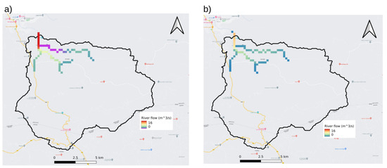
Figure 5.
River flow [] that contributes to the Dechatu River at the forecast point (a) 6 August 2006 at 13 h; (b) 6 August 2006 at 14 h.
The hourly simulated stream discharge at the Dechatu River with default and selected best parameters are compared in Figure 6a. The simulation with the default parameters was found to be non-responsive to the available precipitation in the domain. The stream discharge is almost zero throughout the simulation period due to the higher magnitudes of the default REFKDT and DKSAT values; there is a significant augmentation in the soil column’s infiltration capacity. This, in turn, contributes to a decrease in surface runoff. On the other hand, the simulation with calibrated parameters displayed to have higher volume of discharge immediately after largest precipitation is observed in the domain (Figure 6a). As a result of fine-tuning the parameters detailed in Table 3, the simulations have effectively yielded improved outcomes, notably in accurately representing the initiation and conclusion of flood events within the river basin, as depicted in Figure 6.
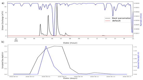
Figure 6.
(a) WRF-Hydro hourly stream discharge [] of default and calibrated parameters compared with the rainrate [] obtained from ERA5 data for the period of 1–15 August 2006; (b) daily simulated flow depth [m] is compared with observed flow depth [m] for the duration of 1–15 August 2006.
Figure 6b compares the daily observed and simulated flow depth (the simulation uses the calibrated parameters). The maximum flow depth of both the simulated and observed happens to occur on a similar date. This means that the simulated flow depth managed to identify the occurrence of the flash flood. However, the simulation underestimated the depth of the flash flood compared with the observed flow depth. It is critical to note that, unlike dynamical variables, the precipitation field in ERA5 reanalysis is greatly influenced by the physical parametrization in the ECMWF model and, hence, is related to the quality of short-range numerical weather prediction output. A comparison (not shown) indicated that ERA5 precipitation amounts are lower than those of WRFDEI (a bias adjusted precipitation data generated using the same methodology as the widely used WATCH Forcing Data (WFD)) over the study region, highlighting the importance of accurate precipitation forcing.
Having observed the enhanced performance of WRF-Hydro resulting from the modification of parameter settings described above, we proceeded to employ the calibrated model to investigate two recent extreme cases, which occurred in March 2005 and April 2007. The subsequent subsections will present a comprehensive analysis of the meteorological precursors, as well as a detailed account of the WRF-Hydro simulation results.
3.2. Case Study I (March 2005)
3.2.1. Extreme Precipitation Event and Its Association with Circulation Anomalies
The anomalous heavy precipitation event of March 2005 affected most of the eastern and central Ethiopia, but its most devastating impact was over Dire Dawa city. Figure 7 shows the spatial distribution of precipitation amount for the 17–21 March 2005 and its deviation from the corresponding long-term average. It is clear that the precipitation amount in 2005 is much higher than the corresponding climatological values for most regions, including over Dire Dawa.
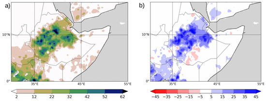
Figure 7.
(a) CHIRPS precipitation (mm) [17–20] March 2005; (b) CHIRPS precipitation anomaly [17–20] March 2005—Climatology [1991–2020].
This extreme precipitation event was associated with notable anomalies in oceanic and atmospheric circulation features. Although ENSO condition was not strong, the sea surface temperature anomaly (SSTa) distribution during the heavy rainfall event is characterized by a dipole pattern of sea surface temperature anomaly over the southwestern Indian Ocean (Figure 8a). The dipole pattern is composed of a warm SST anomaly north of Madagascar and a cold SST anomaly over Mascarene. It is interesting to note that this dipole pattern of SST is co-located with a dipole pattern of sea-level pressure anomaly, with stronger than normal Mascarene high and negative SLP anomalies over the north of Madagascar, as shown in Figure 8c. Such intensification of a high pressure system over Mascarene is in line with strengthening of southerly influx of moisture from the Indian Ocean to eastern Africa, as shown in Figure 9a. It is also important to note the unusual extended high pressure anomaly centered over the Mediterranean Sea (which is higher than the Azores high), but its extent reaches over northeast Africa and the Middle East. These cause northeasterly anomalies from north Africa, and easterly anomalies over the northern Indian Ocean converge with the southeasterly anomaly from southern Indian Ocean, as shown in the low-level circulation anomaly (Figure 9a,b). Upper-level circulation features (Figure 9) revealed that the sub-tropical westerly jet stream is intensified and shifted southward over northern Africa during extreme precipitation events. This upper-level anomalous circulation is conducive to create upper-level divergence. These upper- and lower-level circulation anomalies are in line with those reported in [42].
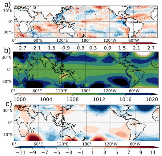
Figure 8.
(a) OI SST anomaly [°C], [17–21] March 2005—climatology [1991–2020]; (b) ERA5 SLP [hPa] [17–21] March 2005; (c) ERA5 SLP anomaly [hPa] [17–21] March 2005—climatology [1991–2020].
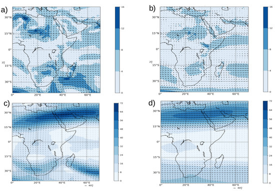
Figure 9.
(a) Wind at 850 hPa [ms] for 17–21 March; (b) wind at 850 hPa [ms] for 17–21 March 2005—[1991–2020] climatology; (c) wind at 200 hPa [ms] for 17–21 March 2005; (d) wind at 200 hPa [ms] for 17–21 March 2005—[1991–2020] climatology.
3.2.2. WRF-Hydro Simulation for the Case Study of March 2005
The calibrated WRF-Hydro model is configured to investigate two well-known flood events in Dire Dawa. The first case study considers one of the flood events that occurred on 20 March 2005 [11].
Figure 10a–h indicate the spatial distribution of the forcing precipitation field in the inner domain, where a higher-resolution (1 km) hydrological model is conducted. Based on the forcing field, the precipitation that triggered the flood began on 17 March, with a precipitation amount of 0.003–0.004 mm/s in the western part of the domain (Figure 10b). Subsequently, on 18 March, there was widespread precipitation across the entire domain, with a precipitation amount of 0.006 mm/s in the highland region (Figure 10c). On March 19th, there was further intense precipitation on the western edge of the domain, but a substantial amount of precipitation still fell over the highland area (Figure 10d). The highland regions received a significant amount of rainfall over the next two days, i.e., 20 and 21 March, before the precipitation finally ceased (Figure 10e–h).
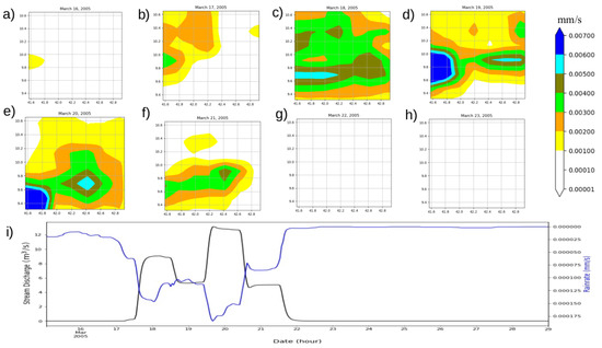
Figure 10.
Spatial distribution of daily cumulative precipitation [mms] obtained from ERA5 reanalysis precipitation data for duration of 15–30 March 2005, (a–h), respectively. (i) Time series with running mean of 24 h of stream discharge [] (black) and rainrate [mms] (blue) for the period of 15–30 March 2005.
In Figure 10i, we calculated the average precipitation solely for the highland region. The simulated stream discharge began to rise on 17 March 2005 in response to the corresponding increase in input precipitation forcing. The peak stream discharge at the forecast point coincided with the highest mean precipitation in the domain, as depicted in Figure 10i. In this instance, the simulation successfully replicated the flood event of 20 March 2005.
The comparison of the observed and simulated maximum flow depths showed that the flash flood that occurred on 20 March 2005 was precisely detected by the simulated maximum flow depth (Figure 11). Subsequently, after the flood event, the flow depths of both the simulated and observed data decreased rapidly. However, compared to the measured flow depth, the simulation underestimated the depth of the flash flood; it should be noted that this was also the case during the flood of August 2006. The NSE value determined for this time period is discovered to be 0.56, which is within the acceptable range of the hydrological analysis [56].
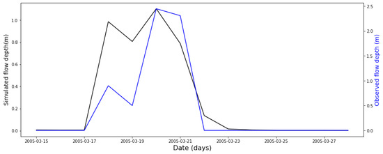
Figure 11.
Daily simulated flow depth [m] is compared with observed flow depth [m] for the duration of 15–29 March 2005.
3.3. Case Study II (April 2007)
3.3.1. Climatological Perspectives for the Case of April 2007
During 12–16 April 2007, heavy precipitation events occurred over eastern Ethiopia (Figure 12). The precipitation amount exceeds the climatological values by over 20 mm/day. Most of the heavy precipitation events occurred over Dire Dawa, leading to flash flood and a high level of Dechatu River, with dramatic consequences for people and infrastructure. One of the aims of this section is to identify the circulation type associated with the flood events.
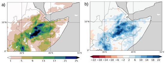
Figure 12.
(a) CHIRPS precipitation (mm) [12–16] April 2007; (b) CHIRPS precipitation anomaly [12–16] April 2007—Climatology [1991–2020].
The notable SST anomalies during the April 2007 flood event include negative anomalies over the Nino 1+2 region and warming anomalies over the northwest Indian Ocean (Figure 13). The sea-level pressure anomalies include weakening of the high pressure system over the Arabian Sea. However, positive anomalies are noted over Mascarene and over northeastern Sudan and Egypt. These patterns of positive sea level pressure anomalous are in line with the northerly flow anomalies over the Red Sea and southerly flow anomalies from the southern Indian Ocean, which suggest an intensification of moisture influx to eastern and southern Ethiopia. At the upper level, similar to the March 2005 case, the tropical westerly jet is shifted southward and also strengthened compared to climatological values, which favors an upper-level divergence (Figure 14).
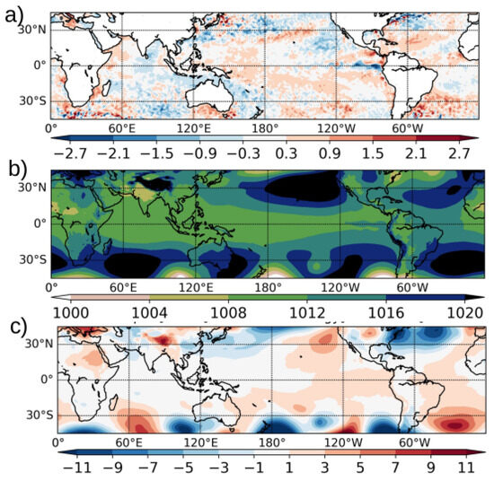
Figure 13.
(a) OI SST anomaly [°C], [12–16] April 2007—climatology [1991–2020]; (b) ERA5 SLP [hPa] [12–16] April 2007; (c) ERA5 SLP anomaly [hPa] [12–16] April 2007—climatology [1991–2020].
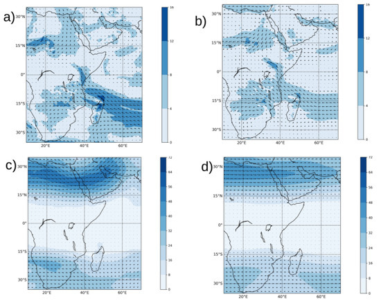
Figure 14.
(a) Wind at 850 hPa [ms] for 12–16 April; (b) wind at 850 hPa [ms] for 12–16 April 2007—[1991–2020] climatology; (c) wind at 200 hPa [ms] for 12–16 April 2007; (d) wind at 200 hPa [ms] for 12–16 April 2007—[1991–2020] climatology.
3.3.2. WRF-Hydro Simulation for the Case Study of April 2007
The other flood event that is considered in this case study happened on 12 April 2007 [11]. The spatial distribution of precipitation in the inner domain displays relatively less precipitation (less than 0.006 mm/s) on the specified date, as shown in Figure 15c. Following that, widespread precipitation occurred across the entire domain on 13 April 2007, with a precipitation amount of 0.006 mm/s in the highland region (Figure 15d). On 14 April, there was further intense precipitation throughout the domain (Figure 15e). The highland regions experienced significant rainfall for the next two days, i.e., 15 and 16 April, before the precipitation eventually stopped (Figure 15f–h).
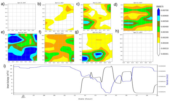
Figure 15.
Spatial distribution of daily cumulative precipitation obtained from ERA5 reanalysis precipitation data [mms] for duration of 5 April to 19 March 2007, (a–h), respectively. (i) Time series with running mean of 24 h of stream discharge [m] (black) and rainrate (blue) for the period of 5–19 April 2007.
Figure 15i indicate an increase in the flow discharge at the Dechatu River forecast point on 12 April 2007. In this case, the model seems to detect the signature of the flood event even if the signal from the input data is not that strong. Unlike our first case study, the representation of the flood event is not exactly on the same day as that of the historical recorded flood event [11]. The WRF-Hydro indicates the highest stream discharge on 14 April 2007, which means it is off by two days when compared to the historical data. The input precipitation ERA5 data (Figure 15e) might play a critical role in delaying the representation of the flood event in the hydrological model.
The model was able to replicate the timing of the flood event by accurately simulating the onset and cessation of the flood event. Specifically, the simulated maximum flow depth started increasing on the same day as the observed data and decreased on a similar day as the observed data. However, the simulation results indicated a discrepancy in the detection of the flash flood that took place on 12 April 2007. Figure 16 revealed a two-day gap between the peak of the observed and simulated flow depth. As in the previous case study, the simulation underestimated the depth of the flash flood, which may be attributed to the ERA5 input data. Nevertheless, the NSE value calculated for this period is 0.66, which falls within the acceptable range of the hydrological analysis [56].
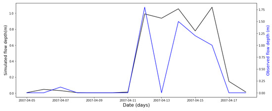
Figure 16.
Daily simulated flow depth [m] is compared with observed flow depth [m] for the duration of 5–18 April 2007.
3.4. Limitations of the Simulations
One constraint of this study pertains to its heavy reliance on ERA5 precipitation data for simulation input. Any inaccuracies or discrepancies within the ERA5 dataset can cascade through the hydrological modeling process. Furthermore, the somewhat coarse spatial resolution of ERA5 data might struggle to accurately capture smaller-scale, intense precipitation events. The model’s tendency to underestimate peak flood depths could potentially be linked to the limitations in ERA5 precipitation data quality.
Another limitation revolves around the relatively short simulation period. Extending the simulations to encompass multiple seasons or years would offer a more comprehensive assessment of the model’s performance across a wider array of hydrological scenarios. Lastly, although the 1 km model resolution is fairly robust, achieving a sub-kilometer resolution could enhance the model’s ability to accurately depict small-scale topographical features that exert influence on flooding dynamics.
Despite these factors, the simulations successfully depicted the beginning, peak and end of the flood event with accuracy, making them a valuable demonstration of flood event modeling within the region of Dire Dawa, Ethiopia.
4. Summary and Conclusions
In terms of both human impacts and economic losses, flooding stands out as one of the most significant types of natural disasters [57,58]. In many parts of Africa, floods have caused damage to crops, loss of infrastructure and worsened the spread of water-borne diseases. Furthermore, the frequency and intensity of flood events have increased in recent decades [3]. Better understanding of flooding mechanisms and hydrometeorological linkages aids disaster preparedness and planning. Model simulations can identify vulnerable areas and conditions prone to severe flooding.
Therefore, it is crucial to develop a modeling capability and understanding of flood events for early warning systems. With this goal in mind, a WRF-Hydro model has been configured at a 1 km (250 m) resolution over the Horn of Africa to simulate major flood events in the eastern Ethiopia domain.
Multiple sensitivity experiments have been performed with the WRF-Hydro model to comprehend and portray the impact of different parameter values on streamflow response. These experiments were conducted for August 2006 events, and the most sensitive parameters are found to be hydraulic conductivity, surface infiltration coefficient and saturated volumetric soil moisture. The result of these experiments aided in obtaining suitable parameter values of 0.1 for infiltration runoff, 1.5 for hydraulic soil conductivity and 1.0 for saturated volumetric soil moisture. Using the adjusted parameters in the experiments, the model is able to accurately represent the crucial aspects of the flood event, such as the start, peak and end timings.
To evaluate the performance of the configured WRF-Hydro model, we conducted tests using data from two flood episodes that occurred in March 2005 and April 2007. The results revealed NSE values of 0.56 for March 2005 and 0.66 for April 2007 flood events. In addition, the WRF-Hydro model demonstrated its ability to capture the timing and peak levels of the flood events. However, it was observed that the model tends to underestimate the magnitude of the floods. This suggests that, while the model was effective in simulating the general behavior and characteristics of the flood events, there is a room for future improvement for accurately reproducing the exact magnitude of the flooding.
Furthermore, composite analysis has been performed using the ERA5 reanalysis dataset to understand the atmospheric precursors. The results revealed that, despite the absence of a strong ENSO signal, these flood events are associated with regional SST and atmospheric circulation that favours convergence of wind at low level and southward shift of the sub-tropical upper level jet stream, which rise to divergence at the upper level over eastern Africa. All of these are conducive to the generation of heavy precipitation amounts that are much higher than the climatological values.
The promising findings suggest that integrating the WRF-Hydro model into the regional and national operational centers would be beneficial to enhance their flood monitoring and early warning systems. As a future project, we will explore the impact of using higher-resolution configuration, a better routing scheme and further tuning of the coupled WRF-Hydro model. Additionally, we will conduct further sensitivity experiments by incorporating observed precipitation data as well as the impact of different rainfall scenarios.
Author Contributions
Conceptualization, A.G.S., G.T.D. and T.D.; methodology, A.G.S. and G.T.D.; software, A.G.S.; validation, A.G.S.; formal analysis, A.G.S. and G.T.D.; investigation, A.G.S. and G.T.D.; resources, T.D.; data curation, B.H.; writing—original draft preparation, A.G.S. writing—review and editing, G.T.D. and T.D.; visualization, A.G.S., G.T.D. and Y.M.Y.; supervision, G.T.D.; project administration, A.G.S.; funding acquisition, T.D. All authors have read and agreed to the published version of the manuscript.
Funding
This research is funded by the International Development Association (IDA) of the World Bank to the Accelerating Impacts of CGIAR Climate Research for Africa (AICCRA) project.
Acknowledgments
This work was supported by Addis Ababa University, and the European Union’s Horizon 2020 program through the CONFER project (grant 869730). GTD is currently affiliated with Environment and Climate Change Canada.
Conflicts of Interest
The authors declare no conflict of interest.
Appendix A
Appendix A.1. Surface Infiltration
is the function of spatially varying precipitation inputs and soil properties. is excess precipitation or through fall from canopy and is given by
where is the water input to the soil surface, and is the model time step in hours (). is calculated depending on the existence of a snow layer, and it accounts for rain water, melting water from the bottom of the snow pack, soil surface dew rate adjusted for frost.
The term is the total soil moisture content that can potentially infiltrate, which depends on soil properties:
where [m] and [] are the thickness and volumetric soil moisture content of the k-th soil layer (k = 1,..., N = 4), respectively, and SMCMAX [] is the saturated volumetric soil moisture content dependent on soil type.
Appendix A.2. Model Performance Evaluation
Appendix A.3. Supplementary Figures
Below are the supplementary figures that offer extra information about the WRF-Hydro simulations and observational analyses.
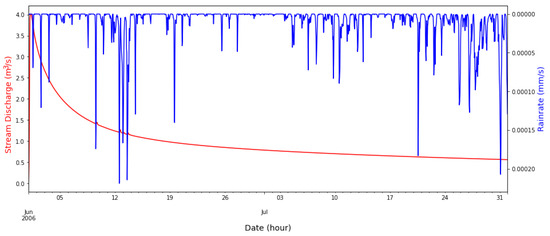
Figure A1.
Stream discharge [] with hourly time step at the outlet of Dechatu River (red); domain mean (D3) rainrate [mms] (blue) for a period of two months (1 June to 31 July 2006).
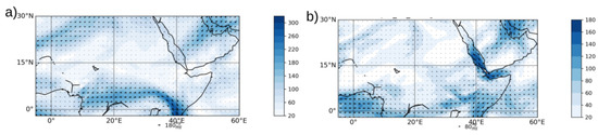
Figure A2.
(a) Integrated moisture flux [] for [12–16] April avg. 2007; (b) integrated moisture flux [] anomaly for [12–16] April avg. 2007—[1991–2020].
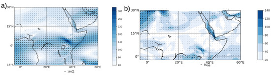
Figure A3.
(a) Integrated moisture flux [] for [17–21] March avg. 2005; (b) integrated moisture flux [] anomaly for [17–21] March avg. 2005—[1991–2020].
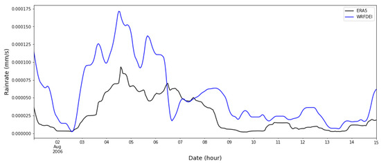
Figure A4.
Time series of precipitation forcing data obtained from ERA5 and WRFDEI (generated using the same methodology as the widely used WATCH Forcing Data).
Table A1.
Summarizes various studies that investigated prediction of flood.
Table A1.
Summarizes various studies that investigated prediction of flood.
| References | Key Findings | Gap Identified |
|---|---|---|
| Maidment 2017 [21] | Presents a conceptual framework to connect information from high-resolution flood forecasting with real-time observations | It is not fully distributed and could not capture surface heterogeneity |
| Camera et al. (2020) [23], Silver et al. (2017) [25], Chowdhury et al. (2023) [26] and Xu et al. (2023) [27] | High-resolution land-surface-based hydrological models are able to simulate the pick, timing and spatial distribution of flood events reasonably | Large-scale atmospheric circulations associated with heavy precipitation were not investigated. All the studies were not conducted in East African region |
| Lahmers et al. (2015) [28] and Lahmers et al. (2019) [24], Cerbelaud et al. (2022) [29] | The uncoupled WRF-Hydro model can accurately simulate streamflow and pick, timing and spatial distribution of flood events when calibrated for specific river basins (Gile River and Babocomari River basins) in southern Arizona, across six watersheds in New Caledonia’s tropical island (SW Pacific) | Investigations into large-scale atmospheric circulations linked to intense precipitation have been limited, and none of the studies have specifically focused on the East African region. |
| Kerandi et al. (2018) [30] | WRF-Hydro used to quantify the terrestrial water balance over the Tana River basin in East | Large-scale atmospheric circulations associated with heavy precipitation were not investigated. |
| Givati et al. (2014) [35] and Krajewski et al. (2017) [34] | WRF-Hydro used operationally for flood forecasting over the US and Israel | Operational flood forecasting was not applied in East African region |
| Shanko et al. (1998) [37], Segele et al. (2009) [36], Diro et al. (2011) [38], Viste and Sorteberg (2013) [40], Zeleke et al. (2017) [41] and Bekele-Biratu et al. (2018) [39] | The dynamics of large-scale climate drivers like the Indian Ocean Dipole and Madden–Julian Oscillation and others can influence heavy precipitation at sub-seasonal and seasonal time scale | Flash flood forecasting was not conducted in these studies |
References
- Diaz, J.H. The public health impact of hurricanes and major flooding. J. La. State Med. Soc. Off. Organ La. State Med. Soc. 2004, 156, 145–150. [Google Scholar]
- Noji, E.K. Natural disasters. Crit. Care Clin. 1991, 7, 271–292. [Google Scholar] [CrossRef] [PubMed]
- Tramblay, Y.; Villarini, G.; Zhang, W. Observed changes in flood hazard in Africa. Environ. Res. Lett. 2020, 15, 1040b5. [Google Scholar] [CrossRef]
- Berghuijs, W.R.; Aalbers, E.E.; Larsen, J.R.; Trancoso, R.; Woods, R.A. Recent changes in extreme floods across multiple continents. Environ. Res. Lett. 2017, 12, 114035. [Google Scholar] [CrossRef]
- Kale, V.S. Is flooding in S outh A sia getting worse and more frequent? Singap. J. Trop. Geogr. 2014, 35, 161–178. [Google Scholar] [CrossRef]
- Shrestha, M.S.; Takara, K. Impacts of floods in South Asia. J. South Asia Disaster Study 2008, 1, 85–106. [Google Scholar]
- FitzGerald, G.; Du, W.; Jamal, A.; Clark, M.; Hou, X.Y. Flood fatalities in contemporary Australia (1997–2008). Emerg. Med. Australas. 2010, 22, 180–186. [Google Scholar] [CrossRef]
- Nations, U. World urbanization prospects: The 2001 revision. Data tables and highlights. In World Urban Prospect 2003 Revis; 2002; pp. 1–195. Available online: http://www.megacities.uni-koeln.de/documentation/megacity/statistic/wup2001dh.pdf (accessed on 1 May 2023).
- Alderman, K.; Turner, L.R.; Tong, S. Floods and human health: A systematic review. Environ. Int. 2012, 47, 37–47. [Google Scholar] [CrossRef]
- Di Baldassarre, G.; Montanari, A.; Lins, H.; Koutsoyiannis, D.; Brandimarte, L.; Blöschl, G. Flood fatalities in Africa: From diagnosis to mitigation. Geophys. Res. Lett. 2010, 37. [Google Scholar] [CrossRef]
- Billi, P.; Alemu, Y.T.; Ciampalini, R. Increased frequency of flash floods in Dire Dawa, Ethiopia: Change in rainfall intensity or human impact. Nat. Hazards 2015, 76, 1373–1394. [Google Scholar] [CrossRef]
- Erena, S.H.; Worku, H. Flood risk analysis: Causes and landscape based mitigation strategies in Dire Dawa city, Ethiopia. Geoenviron. Disasters 2018, 5, 16. [Google Scholar] [CrossRef]
- Erena, S.H.; Worku, H.; De Paola, F. Flood hazard mapping using FLO-2D and local management strategies of Dire Dawa city, Ethiopia. J. Hydrol. Reg. Stud. 2018, 19, 224–239. [Google Scholar] [CrossRef]
- Demessie, D.A. Assessment of Flood Risk in Dire Dawa Town, Eastern Ethiopia, Using Gis. Ph.D. Thesis, Addis Ababa University, Addis Ababa, Ethiopia, 2007. [Google Scholar]
- Douglas, I.; Alam, K.; Maghenda, M.; Mcdonnell, Y.; McLean, L.; Campbell, J. Unjust waters: Climate change, flooding and the urban poor in Africa. Environ. Urban. 2008, 20, 187–205. [Google Scholar] [CrossRef]
- Olivier, J.G.; Van Aardenne, J.A.; Dentener, F.J.; Pagliari, V.; Ganzeveld, L.N.; Peters, J.A. Recent trends in global greenhouse gas emissions: Regional trends 1970–2000 and spatial distributionof key sources in 2000. Environ. Sci. 2005, 2, 81–99. [Google Scholar] [CrossRef]
- Du, H.; Alexander, L.V.; Donat, M.G.; Lippmann, T.; Srivastava, A.; Salinger, J.; Kruger, A.; Choi, G.; He, H.S.; Fujibe, F.; et al. Precipitation from persistent extremes is increasing in most regions and globally. Geophys. Res. Lett. 2019, 46, 6041–6049. [Google Scholar] [CrossRef]
- Myhre, G.; Alterskjær, K.; Stjern, C.W.; Hodnebrog, Ø.; Marelle, L.; Samset, B.H.; Sillmann, J.; Schaller, N.; Fischer, E.; Schulz, M.; et al. Frequency of extreme precipitation increases extensively with event rareness under global warming. Sci. Rep. 2019, 9, 16063. [Google Scholar] [CrossRef]
- Coumou, D.; Robinson, A. Historic and future increase in the global land area affected by monthly heat extremes. Environ. Res. Lett. 2013, 8, 034018. [Google Scholar] [CrossRef]
- Zhang, X.; Alexander, L.; Hegerl, G.C.; Jones, P.; Tank, A.K.; Peterson, T.C.; Trewin, B.; Zwiers, F.W. Indices for monitoring changes in extremes based on daily temperature and precipitation data. Wiley Interdiscip. Rev. Clim. Chang. 2011, 2, 851–870. [Google Scholar] [CrossRef]
- Maidment, D.R. Conceptual framework for the national flood interoperability experiment. JAWRA J. Am. Water Resour. Assoc. 2017, 53, 245–257. [Google Scholar] [CrossRef]
- Usman, M.; Ndehedehe, C.E.; Farah, H.; Ahmad, B.; Wong, Y.; Adeyeri, O.E. Application of a Conceptual Hydrological Model for Streamflow Prediction Using Multi-Source Precipitation Products in a Semi-Arid River Basin. Water 2022, 14, 1260. [Google Scholar] [CrossRef]
- Camera, C.; Bruggeman, A.; Zittis, G.; Sofokleous, I.; Arnault, J. Simulation of extreme rainfall and streamflow events in small Mediterranean watersheds with a one-way-coupled atmospheric–hydrologic modelling system. Nat. Hazards Earth Syst. Sci. 2020, 20, 2791–2810. [Google Scholar]
- Lahmers, T.M.; Gupta, H.; Castro, C.L.; Gochis, D.J.; Yates, D.; Dugger, A.; Goodrich, D.; Hazenberg, P. Enhancing the structure of the WRF-hydro hydrologic model for semiarid environments. J. Hydrometeorol. 2019, 20, 691–714. [Google Scholar] [CrossRef]
- Silver, M.; Karnieli, A.; Ginat, H.; Meiri, E.; Fredj, E. An innovative method for determining hydrological calibration parameters for the WRF-Hydro model in arid regions. Environ. Model. Softw. 2017, 91, 47–69. [Google Scholar]
- Chowdhury, M.E.; Islam, A.S.; Lemans, M.; Hegnauer, M.; Sajib, A.R.; Pieu, N.M.; Das, M.K.; Shadia, N.; Haque, A.; Roy, B.; et al. An efficient flash flood forecasting system for the un-gaged Meghna basin using open source platform Delft-FEWS. Environ. Model. Softw. 2023, 161, 105614. [Google Scholar] [CrossRef]
- Xu, Y.; Jiang, Z.; Liu, Y.; Zhang, L.; Yang, J.; Shu, H. An adaptive ensemble framework for flood forecasting and its application in a small watershed using distinct rainfall interpolation methods. Water Resour. Manag. 2023, 37, 2195–2219. [Google Scholar] [CrossRef]
- Lahmers, T.; Castro, C.L.; Gupta, H.V.; Gochis, D.J.; ElSaadani, M. Optimization of precipitation and streamflow forecasts in the southwest Contiguous US for warm season convection. In Proceedings of the AGU Fall Meeting Abstracts, San Francisco, CA, USA, 14–18 December 2015; Volume 2015, p. H53A-1650. [Google Scholar]
- Cerbelaud, A.; Lefèvre, J.; Genthon, P.; Menkes, C. Assessment of the WRF-Hydro uncoupled hydro-meteorological model on flashy watersheds of the Grande Terre tropical island of New Caledonia (South-West Pacific). J. Hydrol. Reg. Stud. 2022, 40, 101003. [Google Scholar] [CrossRef]
- Kerandi, N.; Arnault, J.; Laux, P.; Wagner, S.; Kitheka, J.; Kunstmann, H. Joint atmospheric-terrestrial water balances for East Africa: A WRF-Hydro case study for the upper Tana River basin. Theor. Appl. Climatol. 2018, 131, 1337–1355. [Google Scholar] [CrossRef]
- Senatore, A.; Furnari, L.; Mendicino, G. Impact of high-resolution sea surface temperature representation on the forecast of small Mediterranean catchments’ hydrological responses to heavy precipitation. Hydrol. Earth Syst. Sci. 2020, 24, 269–291. [Google Scholar] [CrossRef]
- Papaioannou, G.; Vasiliades, L.; Loukas, A.; Alamanos, A.; Efstratiadis, A.; Koukouvinos, A.; Tsoukalas, I.; Kossieris, P. A flood inundation modeling approach for urban and rural areas in lake and large-scale river basins. Water 2021, 13, 1264. [Google Scholar] [CrossRef]
- Yucel, I.; Onen, A.; Yilmaz, K.; Gochis, D. Calibration and evaluation of a flood forecasting system: Utility of numerical weather prediction model, data assimilation and satellite-based rainfall. J. Hydrol. 2015, 523, 49–66. [Google Scholar] [CrossRef]
- Krajewski, W.F.; Ceynar, D.; Demir, I.; Goska, R.; Kruger, A.; Langel, C.; Mantilla, R.; Niemeier, J.; Quintero, F.; Seo, B.C.; et al. Real-time flood forecasting and information system for the state of Iowa. Bull. Am. Meteorol. Soc. 2017, 98, 539–554. [Google Scholar] [CrossRef]
- Givati, A.; Sapir, G. Simulating 1% Probability Hydrograph at the Ayalon Basin Using the HEC-HMS; Special Hydrological Report; Israel Hydrological Service: Jerusalem, Israel, 2014. [Google Scholar]
- Segele, Z.T.; Lamb, P.J.; Leslie, L.M. Large-scale atmospheric circulation and global sea surface temperature associations with Horn of Africa June–September rainfall. Int. J. Climatol. J. R. Meteorol. Soc. 2009, 29, 1075–1100. [Google Scholar] [CrossRef]
- Shanko, D.; Camberlin, P. The effects of the Southwest Indian Ocean tropical cyclones on Ethiopian drought. Int. J. Climatol. J. R. Meteorol. Soc. 1998, 18, 1373–1388. [Google Scholar] [CrossRef]
- Diro, G.; Grimes, D.I.F.; Black, E. Teleconnections between Ethiopian summer rainfall and sea surface temperature: Part I—Observation and modelling. Clim. Dyn. 2011, 37, 103–119. [Google Scholar] [CrossRef]
- Bekele-Biratu, E.; Thiaw, W.M.; Korecha, D. Sub-seasonal variability of the Belg rains in Ethiopia. Int. J. Climatol. 2018, 38, 2940–2953. [Google Scholar] [CrossRef]
- Viste, E.; Sorteberg, A. Moisture transport into the Ethiopian highlands. Int. J. Climatol. 2013, 33, 249–263. [Google Scholar] [CrossRef]
- Zeleke, T.T.; Giorgi, F.; Diro, G.; Zaitchik, B. Trend and periodicity of drought over Ethiopia. Int. J. Climatol. 2017, 37, 4733–4748. [Google Scholar] [CrossRef]
- Diro, G.T.; Grimes, D.; Black, E. Large scale features affecting Ethiopian rainfall. In African Climate and Climate Change; Springer: Berlin/Heidelberg, Germany, 2011; pp. 13–50. [Google Scholar]
- Austin, G.L.; Dirks, K.N. Topographic effects on precipitation. In Encyclopedia of Hydrological Sciences; Wiley Online Library: Hoboken, NJ, USA, 2006. [Google Scholar]
- Hersbach, H.; Dee, D. ERA5 reanalysis is in production. ECMWF Newsl. 2016, 147. Available online: https://www.ecmwf.int/en/newsletter/147/news/era5-reanalysis-production (accessed on 1 March 2022).
- Funk, C.; Peterson, P.; Landsfeld, M.; Pedreros, D.; Verdin, J.; Shukla, S.; Husak, G.; Rowland, J.; Harrison, L.; Hoell, A.; et al. The climate hazards infrared precipitation with stations—A new environmental record for monitoring extremes. Sci. Data 2015, 2, 150066. [Google Scholar] [CrossRef]
- Schneider, U.; Becker, A.; Finger, P.; Meyer-Christoffer, A.; Ziese, M.; Rudolf, B. GPCC’s new land surface precipitation climatology based on quality-controlled in situ data and its role in quantifying the global water cycle. Theor. Appl. Climatol. 2014, 115, 15–40. [Google Scholar] [CrossRef]
- Amatulli, G.; Domisch, S.; Tuanmu, M.N.; Parmentier, B.; Ranipeta, A.; Malczyk, J.; Jetz, W. A suite of global, cross-scale topographic variables for environmental and biodiversity modeling. Sci. Data 2018, 5, 180040. [Google Scholar] [CrossRef] [PubMed]
- Danielson, J.J.; Gesch, D. Global Multi-Resolution Terrain Elevation Data 2010 (GMTED2010); US Department of the Interior, US Geological Survey: Reston, VA, USA, 2011; p. 26. [Google Scholar]
- Jarvis, A.; Reuter, H.I.; Nelson, A.; Guevara, E. Hole-filled seamless SRTM data V3. International Centre for Tropical Agriculture (CIAT). 2006. Available online: http://srtm.csi.cgiar.org (accessed on 1 July 2021).
- Skamarock, W.C.; Klemp, J.B.; Dudhia, J.; Gill, D.O.; Liu, Z.; Berner, J.; Wang, W.; Powers, J.G.; Duda, M.G.; Barker, D.M.; et al. A Description of the Advanced Research WRF Model Version 4; National Center for Atmospheric Research: Boulder, CO, USA, 2019; Volume 145, p. 145. [Google Scholar]
- Kim, S.; Shen, H.; Noh, S.; Seo, D.J.; Welles, E.; Pelgrim, E.; Weerts, A.; Lyons, E.; Philips, B. High-resolution modeling and prediction of urban floods using WRF-Hydro and data assimilation. J. Hydrol. 2021, 598, 126236. [Google Scholar] [CrossRef]
- NCEP; FNL. Operational Model Global Tropospheric Analyses, Continuing from July 1999. Res. Data Arch. Natl. Cent. Atmos. Res. Comput. Inf. Syst. Lab. 2000, 10, D6M043C6. [Google Scholar]
- Gochis, D.; Yu, W.; Yates, D. WRF-Hydro Model Technical Description and User’s Guide, Version 3.0. NCAR Technical Document. 120p. Available online: https://ral.ucar.edu/projects/wrf_hydro/technicaldescription-user-guide (accessed on 1 July 2021).
- Schaake, J.C.; Koren, V.I.; Duan, Q.Y.; Mitchell, K.; Chen, F. Simple water balance model for estimating runoff at different spatial and temporal scales. J. Geophys. Res. Atmos. 1996, 101, 7461–7475. [Google Scholar] [CrossRef]
- Chen, F.; Dudhia, J. Coupling an advanced land surface–hydrology model with the Penn State–NCAR MM5 modeling system. Part I: Model implementation and sensitivity. Mon. Weather. Rev. 2001, 129, 569–585. [Google Scholar] [CrossRef]
- Moriasi, D.N.; Arnold, J.G.; Van Liew, M.W.; Bingner, R.L.; Harmel, R.D.; Veith, T.L. Model evaluation guidelines for systematic quantification of accuracy in watershed simulations. Trans. ASABE 2007, 50, 885–900. [Google Scholar] [CrossRef]
- Jonkman, S.N. Global perspectives on loss of human life caused by floods. Nat. Hazards 2005, 34, 151–175. [Google Scholar] [CrossRef]
- Re, M. Natural Catastrophes 2006: Analyses, Assessments; Munich Re Publications: Munich, Germany, 2007. [Google Scholar]
Disclaimer/Publisher’s Note: The statements, opinions and data contained in all publications are solely those of the individual author(s) and contributor(s) and not of MDPI and/or the editor(s). MDPI and/or the editor(s) disclaim responsibility for any injury to people or property resulting from any ideas, methods, instructions or products referred to in the content. |
© 2023 by the authors. Licensee MDPI, Basel, Switzerland. This article is an open access article distributed under the terms and conditions of the Creative Commons Attribution (CC BY) license (https://creativecommons.org/licenses/by/4.0/).