1. Introduction
For many areas, water supply systems can be divided into three subsystems: the “execution system”, “feedback system”, and “decision and control system”. The “execution system” is responsible for producing and conveying water to customers. This subsystem includes facilities such as water plants, pump stations, and pipelines. The “feedback system” provides the running status of the system. It includes the measurement system (such as the SCADA system and the customer call center). The “decision and control system” uses the data obtained from the “feedback system” to make decisions and optimize the water supply system. This optimization involves implementing engineering measures, such as pipe network reconstruction and pump station adjustments. The interrelationships between the three subsystems are depicted in
Figure 1.
Water pressure shortage occurs in water distribution systems owing to factors such as inadequate pipeline transport capacity and pump station pressure. Previous studies have mainly focused on describing water shortage problems without establishing a direct connection to customer demands. For example, Mortula [
1] identified water shortage zones based on the residual chlorine concentration in pipelines and provided insights for developing strategies to mitigate potential shortage issues. Cabrera et al. [
2,
3,
4] optimized water shortage by considering energy consumption and operational losses. The authors introduced performance indices to quantify the energy efficiency of individual pipes within the network and suggested potential improvements for energy optimization. Goel [
5] identified the causes of water shortages using sensor data from a network and enabled efficient water management practices with real-time data analysis. Jeong et al. [
6,
7,
8,
9] utilized indicators such as flow entropy and elasticity index to assess water supply system shortages based on system reliability. The authors reassessed the concept of a resilience index for water distribution networks and proposed an improved index that accounts for the network’s hydraulic characteristics. Jun et al. [
10,
11,
12] attributed water shortages to pipeline issues and calculated the probability of inadequate pressure at the customer nodes. The authors identified cost-effective design and rehabilitation strategies for water distribution networks, considering both technical and financial considerations. When water shortages affect customer water usage, customers file complaints with the water supply company via phone calls. These complaints are recorded as water shortages in the database.
Heat maps have been widely utilized in spatial statistical analyses, offering valuable insights into data visualization and theoretical research. Kim [
13] proposed a method for analyzing spatial and temporal trends in the context of non-directional data, such as disease outbreaks and crime patterns. Fobil et al. [
14,
15,
16] conducted a spatial cluster analysis and visualization of various diseases to uncover spatial clustering characteristics and influencing factors in urban areas. Khalid et al. [
17,
18] investigated the spatial distribution characteristics of urban crime events and identified crime hotspots. Mao [
19] analyzed traffic congestion on urban roads using local and static heat maps, whereas Tang [
20] examined the spatiotemporal distribution of subway passenger flow.
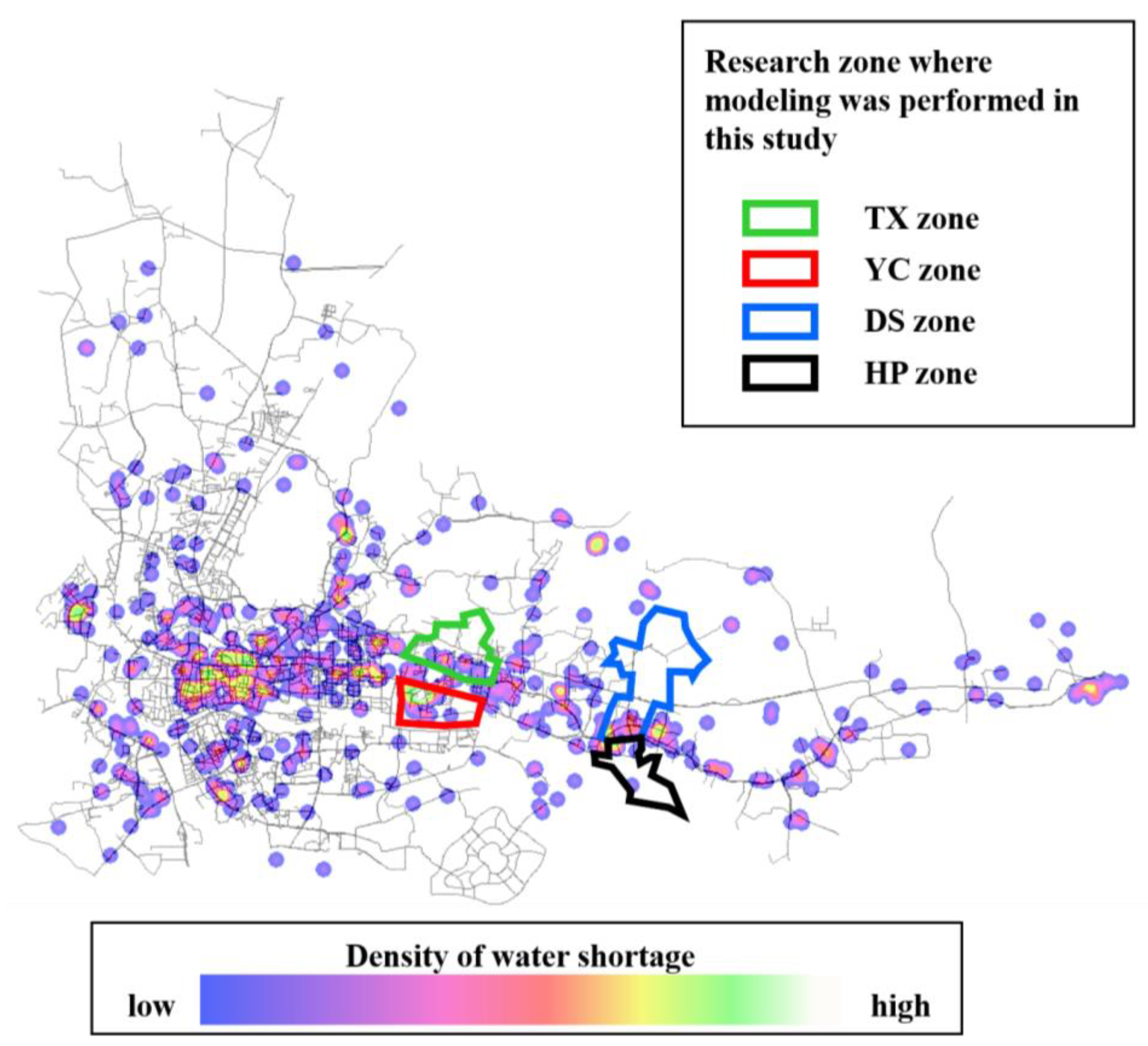
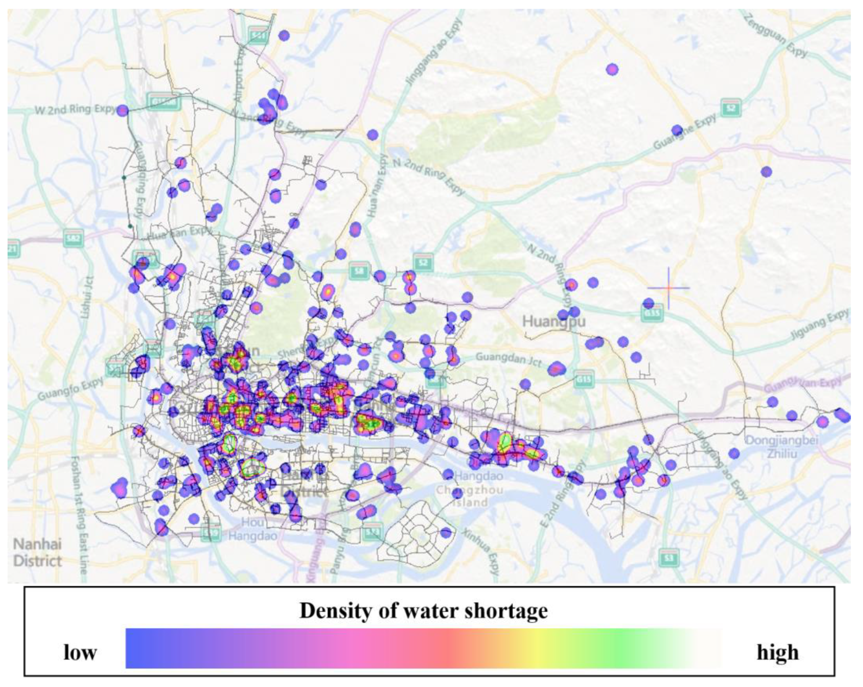
Water shortage records contain valuable information about spatial and temporal characteristics, directly reflecting unsatisfied water demand. Therefore, by incorporating analysis techniques from diverse fields to examine spatiotemporal distribution characteristics, the research capabilities for water shortage issues in water distribution systems can be enhanced. In this study, the authors used a heat map to analyze the distribution of water shortage records in GZ city, as shown in
Figure 2. This heat map only reflects water shortages in the spatial dimension. However, questions remain, such as how much water demand will lead to a water shortage event, or how much water pump station pressure must be increased to alleviate a water shortage. Quantitative descriptions are currently lacking.
The customer service system has not been included in water-supply engineering technology research and is only considered an aspect of customer management. However, in practical operations and management, water supply schedulers often rely on feedback from customer service systems to make decisions. Under most conditions, customer complaints are fuzzy and cannot be analyzed quantitatively as is possible in traditional numerical technology. Water supply dispatchers often rely on their experience to make decisions regarding pump adjustments. This study aimed to establish a relationship between the probability of customer complaints and water supply pressure or flow. First, the entire city was divided into smaller zones, and water shortage records were collected. Second, these records were marked according to the pressure and flow of the water pump stations; the fitted line of the marked points represents the critical pressure-flow conditions when water shortages occur. Subsequently, a statistical model of water shortage was established. In this model, the probability of water shortage is related to the pressure flow at the pump stations. The Boltzmann and Sigmoid functions are in good agreement with the cumulative probability of water shortage.
The parameters in this model were analyzed and exhibited a strong correlation with the pressure requirements of water facilities. The critical service pressure line, combined with the water shortage probability model, can be used as a reference for the operation, control, and reconstruction of water distribution systems.
2. Data Processing and Data Analysis
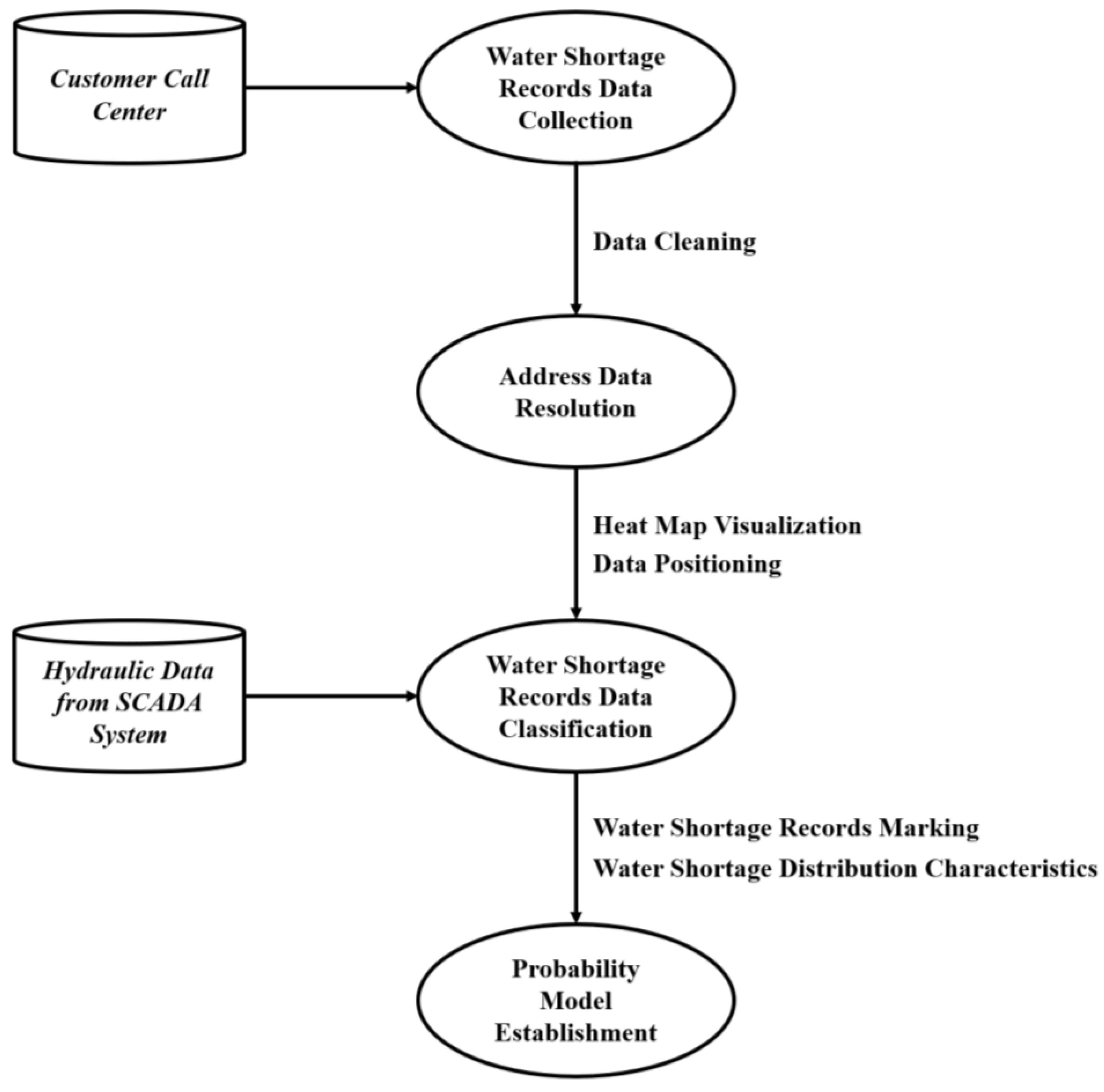
A probability model was developed to assess water shortage events in different zones using data from the customer call center.
Figure 3 shows the implementation of the proposed strategies.
Data processing: The address data of water shortage records were collected from the customer center and subjected to data cleansing. Addresses were matched with a standard address database to ensure a consistent and unified format. Subsequently, the addresses were converted into corresponding spatial coordinates.
Data classification: Zones were divided based on the topological structure of the water distribution system. Water shortage records were classified into their respective zones according to the division results. The pressure and flow data from water plants in the SCADA system corresponded to water shortage records. Through the above steps, the data classification of each zone was completed.
Probability model establishment: For a specific zone under consideration, statistical analysis was conducted on pressure and flow data, with a focus on the occurrences of water shortage events. This analysis aimed at establishing a probability model that quantified the likelihood of future water shortage events based on pressure and flow characteristics within that specific zone.
2.1. Data Processing
2.1.1. Data Collection
The data for this study were obtained from the GZ Company (Guangzhou, China), one of the largest water supply companies in China. The water distribution system operated by the GZ Company covers a vast service area of 518 km2, with a total pipeline length of 5681 km. This extensive network serves a population of approximately 16 million people and represents approximately 2.5% of China’s total daily water supply. The GZ Company has a customer service center for handling customers’ complaints. This center receives many complaints related to insufficient water pressure, ranging from dozens to hundreds each day. The dispatchers and operators investigate these complaints. Based on their analysis, they may make necessary adjustments to satisfy customers’ demands.
2.1.2. Data Standardization and Visualization
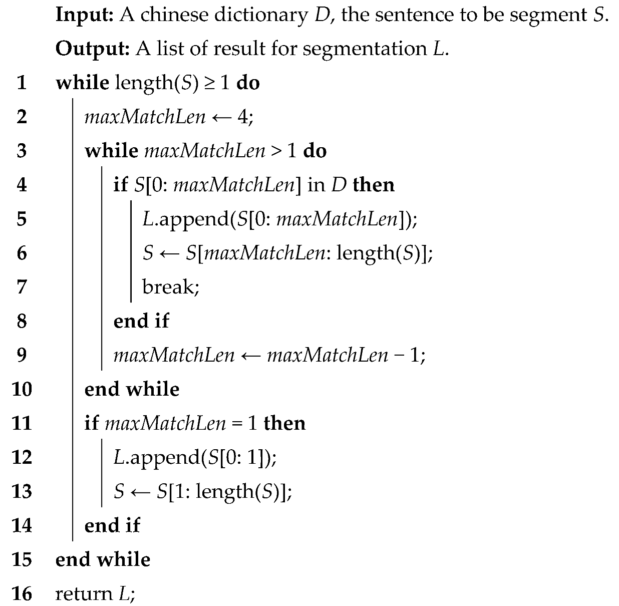
The water shortage records were manually recorded, resulting in inconsistent address formats. These addresses contained various errors, such as incomplete, non-standard, and redundant text. To standardize address formats, it is necessary to split and normalize the given address string. This can be achieved through address segmentation methods, which are similar to Chinese word segmentation algorithms. The Forwards Maximum Match Method (FMM) algorithm is a commonly used Chinese word segmentation algorithm. The FMM algorithm segments the address data by initially splitting the first C characters of the string and searching for corresponding matches in the addresses database. If an initial match is not found, the FMM algorithm removes characters from the end of the string and repeats this matching process iteratively [
21,
22]. Below are the implementation steps of the FMM algorithm:
Define the dictionary: Create a vocabulary database containing the administrative divisions of China (e.g., `dict[]={“Guangzhou”, “Yuexiu District”, “Nonglinxia Road”}').
Read the text to be segmented: Read the Chinese text string to be segmented character by character.
Initialize the pointer: Set a pointer that initially points to the beginning of the string to be segmented.
Start matching: Begin matching the longest word at each step. Follow these specific steps:
Extract a segment of the text to the right of the pointer as the string to be matched.
Compare the string to be matched with the longest word in the dictionary. If there is a match, consider that word as a segmentation result and move the pointer to the end position of that string.
If there is no match, reduce the length of the string to be matched by one character and try to match it with the dictionary again. Repeat this process until a match is found.
Continue matching: Repeat step 4 until the pointer points to the end of the string to be segmented.
Output the result: Output each matched word as a segmentation result.
The algorithms presented in this study have been developed utilizing the Python programming language. Algorithm 1 shows the refinement process of the FMM. By utilizing this iterative matching approach of the FMM algorithm, it was possible to standardize and segment addresses effectively. The resulting standardized addresses provided necessary basic coordinate data for subsequent research purposes without relying on manual correction or human intervention.
| Algorithm 1. Algorithm to Forwards Maximum Match. |
![Water 15 03257 i001]() |
Based on the obtained coordinate data, the visualization of water shortage records was achieved through a heat map. Each water shortage record was represented by a two-dimensional Gaussian circle [
23]. The visualization process was implemented as follows:
where
and
are the coordinates within the calculation buffer zone;
and
are the variances representing the radius of the hotspot; and
and
are the coordinates of the water shortage record.
The coordinate of the water shortage record was , and the water shortage radius was . The range of the calculation buffer zone was defined as and . The water shortage intensity within the calculation buffer zone was represented as the grayscale .
A progressive grayscale band was defined with a range of 255 pixels. By calculating the transparency
the calculation buffer zone was filled with the grayscale [
24].
where
is the transparency of the calculation buffer zone of water shortage record
;
is the grayscale of the calculation buffer zone of water shortage record
;
is the maximum grayscale value; and
is the minimum grayscale value.
The grayscale values of each calculation buffer zone were superimposed. When multiple zones overlapped within the calculation buffer zone, the superimposed grayscale value was increased, resulting in a brighter appearance in the corresponding color [
25].
where
is the resulting transparency of the water shortage record point
after superimposition and
is the transparency of the record point
before superimposition.
The parameters of the two-dimensional Gaussian distribution were adjusted to optimize the presentation of the heat map, ensuring its effectiveness in visualizing the water shortage situation. These parameters were determined by considering the coordinates of the water shortage record data points and the range of the water shortage. If the radius is too small, the representation would only indicate the water shortage locations of individual customers, failing to provide a comprehensive overview of the overall water shortage situation. Conversely, if the radius is too large, the displayed water shortage range may extend to other zones, compromising the accuracy of depicting the localized water shortage situation. To address these concerns, the determination of the heat map radius was adjusted based on the pipe diameter. This adjustment ensured that the heat map point accurately reflects the water shortage situation within the specified zone. As shown in
Figure 4, the heat map visually represents water shortages in the spatial dimension. However, quantitative descriptions are currently lacking. To address this limitation, data classification of water shortage records was performed. The classification process generated a valid dataset that serves as a foundation for subsequent quantitative research.
2.1.3. Data Classification
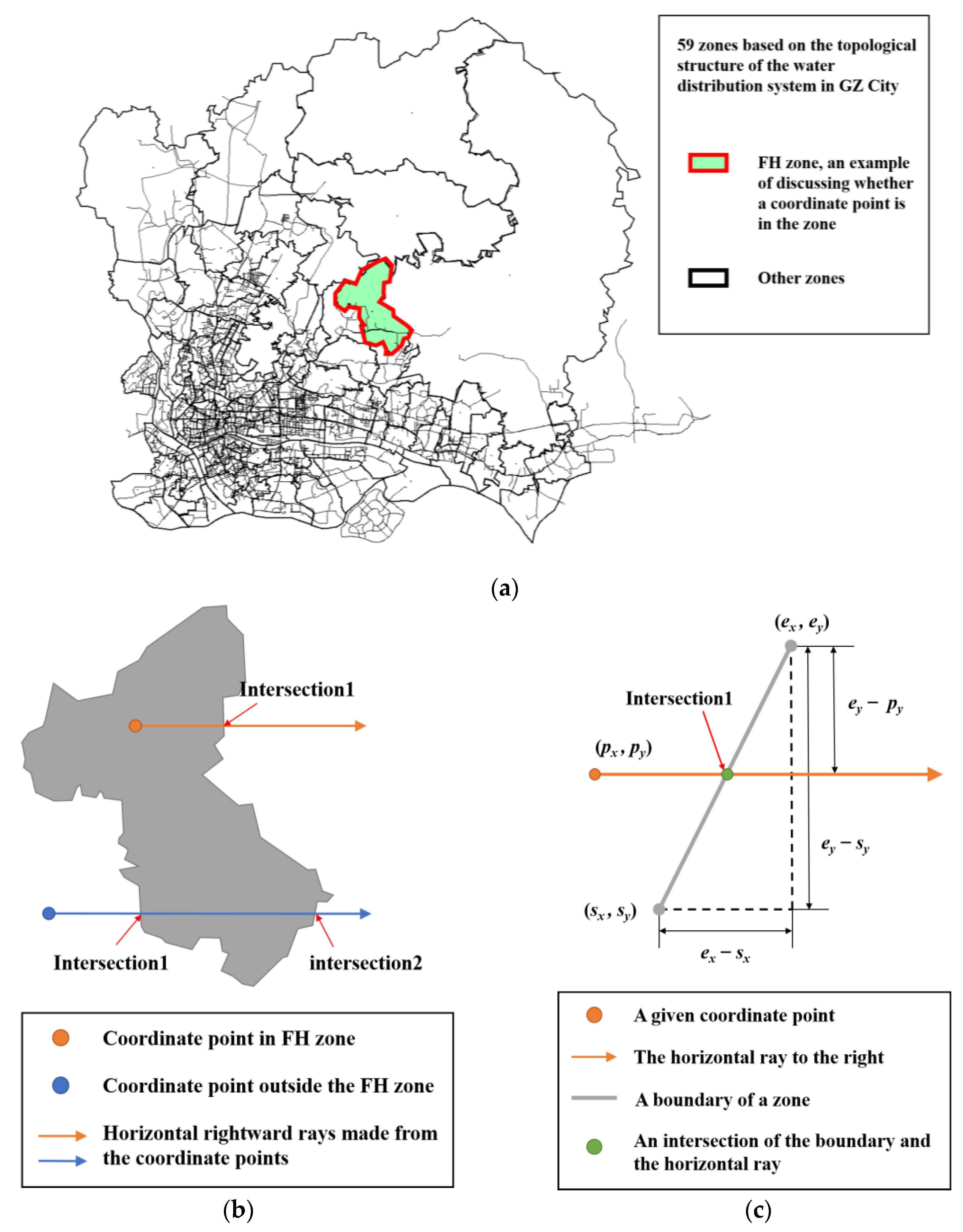
The topological structure of the water distribution system in GZ city is divided into 59 zones. The water shortage records for each zone were counted independently, and the corresponding pressure and flow rate data were obtained from the SCADA database. The Point in Polygon (PIP) problem constitutes a computational geometry challenge primarily concerned with ascertaining the inclusion or exclusion of a given point within a polygonal region. Determining whether a water shortage record falls within a specific zone presents a variation of the PIP problem. The methods for resolving this problem can typically be classified into the following four categories:
Ray Method [
26]: This method involves projecting a ray from a reference point in a standardized direction. The determination is made based on the parity of the number of intersection points between the ray and the boundaries of the zone.
Turning Angle Method [
27]: This method follows the counterclockwise order of vertices along the boundary of the zone polygon. It entails calculating whether positive or negative angles are formed by connecting each vertex with the reference point.
Angle Sum Method [
28]: This method requires calculating all angles formed between each boundary of the zone polygon and the reference point. If their sum equals 360°, then it implies that the reference point lies within that specific zone.
Area Sum Method [
29]: In this method, all triangles’ areas formed by connecting the reference point with the boundaries of the zone polygon are calculated. If their sum is equal to that specific zone’s area, then it indicates that the reference point lies within that particular area.
The computation of multiple zones is intricately complex. The Area Sum Method involves multiple area calculations, rendering it a more intricate approach. Approaches that incorporate angle calculations, such as the Turning Angle Method and Angle Sum Method, necessitate the utilization of inverse trigonometric functions and entail substantial computational effort. The Ray Method entails evaluating the intersection points along each boundary of a polygon through iterative processes. However, within the Ray Method, many cases can be eliminated through straightforward coordinate comparison alone [
30]. Consequently, this study employed the Ray Method to determine the location of water shortage records.
As shown in
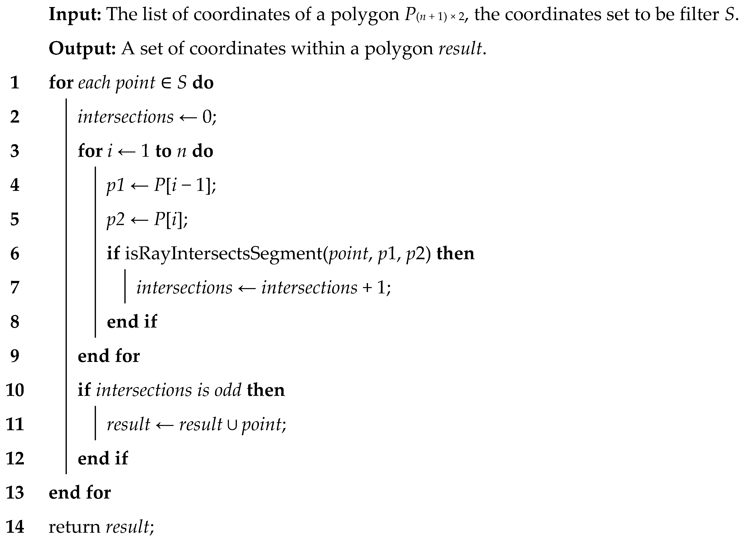
Figure 5, a given coordinate point was assigned to represent the location of a water shortage record. A horizontal ray was projected towards the right direction. The intersections between this ray and each boundary of the zone polygon were computed. If the total count of intersections was an odd number, it indicated that the water shortage point was positioned within the zone. Conversely, if the count of intersections was an even number, it signified that the water shortage point was located outside the zone. Algorithm 2 shows the refinement process of the Ray Method.
The Ray Method crucially relies on the determination of intersections between the ray and each boundary. Equation (4) expresses that the proportional relationship within the triangle was essential. The position of the intersection point relative to the reference point was determined, as depicted in
Figure 5.
(the intersection point is located to the right of the reference point) indicates that the point lies within the zone. Conversely,
(the intersection point is located to the left of the reference point) indicates that the point lies outside the zone.
where
is the distance from the start point to the intersection point;
and
are the coordinates of the upper endpoint of the boundary;
and
are the coordinates of the lower endpoint of the boundary; and
and
are the coordinates of the start point.
| Algorithm 2. Algorithm to filtering points inside a polygon. |
![Water 15 03257 i002]() |
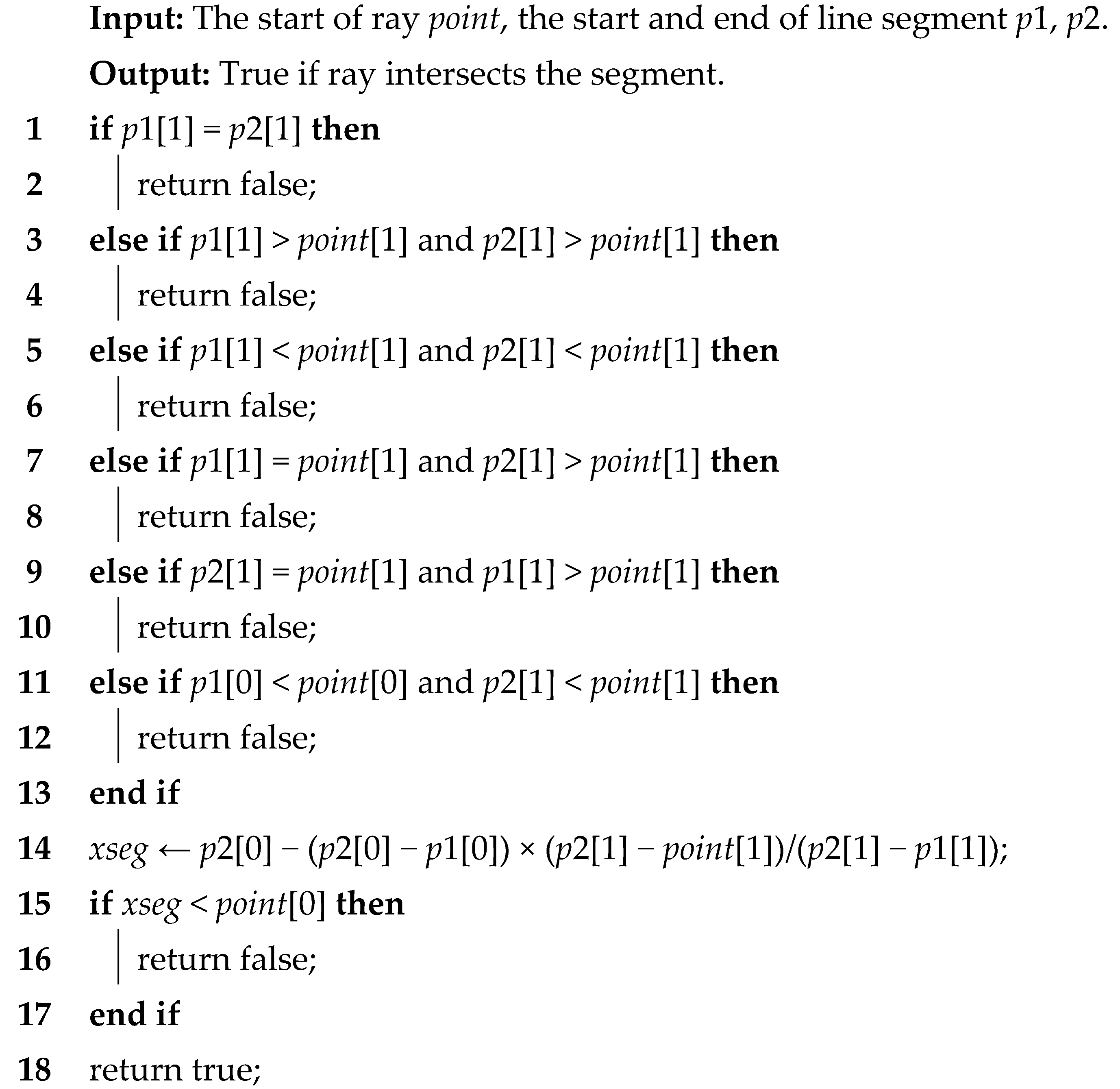
To simplify the computational process of the algorithm, a preliminary step is introduced to identify and exclude cases where the ray and boundary do not intersect. This step helps eliminate cases such as parallel or overlapping ray and boundary, boundary located above or below the ray, ray passing through the lower endpoint of the boundary, and boundary located to the left of the ray. These non-intersecting cases can be determined through simple coordinate comparisons. By eliminating these non-intersecting cases, the subsequent intersection point determination becomes much simpler. It can be achieved by utilizing the proportional relationships within a triangle to assess the position of the start point. Algorithm 3 outlines the refined process, considering these optimizations and simplifications.
The algorithms mentioned above were executed In a loop for each boundary of every zone. This process enabled the collection of water shortage records data for each zone and SCADA data for the water plants. A reasonable dataset is beneficial for revealing the patterns and characteristics of water shortages in urban water distribution systems. This study has organized the water shortage zones in GZ city and completed the data classification through the above analysis. This dataset was used for the subsequent statistical analyses.
| Algorithm 3. isRayIntersectsSegment (point, p1, p2). |
![Water 15 03257 i003]() |
2.2. Data Analysis
Regional water shortage events result from multiple factors such as insufficient pump station pressure, pipeline maintenance, and unpredictable disturbances. However, describing this event using a simple mathematical formula is difficult. The water supply pressure of the pump station and the water consumption of the pipeline network are the most critical factors that cause regional water shortages, whereas other factors can be classified as unpredictable disturbances. The author marked the pressure and flow on the day a shortage occurs. It is helpful to clarify the statistical characteristics of water-shortage events. The subsequent analysis was based on this finding. The YC zone has one of the highest numbers of shortage records, and a shortage hotspot is marked on the heat map (
Figure 2). In this section, the YC zone is used as an example to describe the procedure for analyzing the statistical correlation between the water shortage pressure and the total water distribution demand. In this study, OriginPro 2023b was used for modeling.
2.2.1. Marking of Water Shortage Records
The relationship between the head loss (Δ
H) and the square of the water demand (
Q2) can be expressed as a linear function. The water pump station increases the pressure to satisfy the customer demand. In this study, the daily water pressure (
H) and flow rate (
Q, which represents the water demand) were normalized based on the annual average pressure (
H0) and flow rate (
Q0). These normalized data were plotted with coordinates
H/
H0 − (
Q/
Q0)
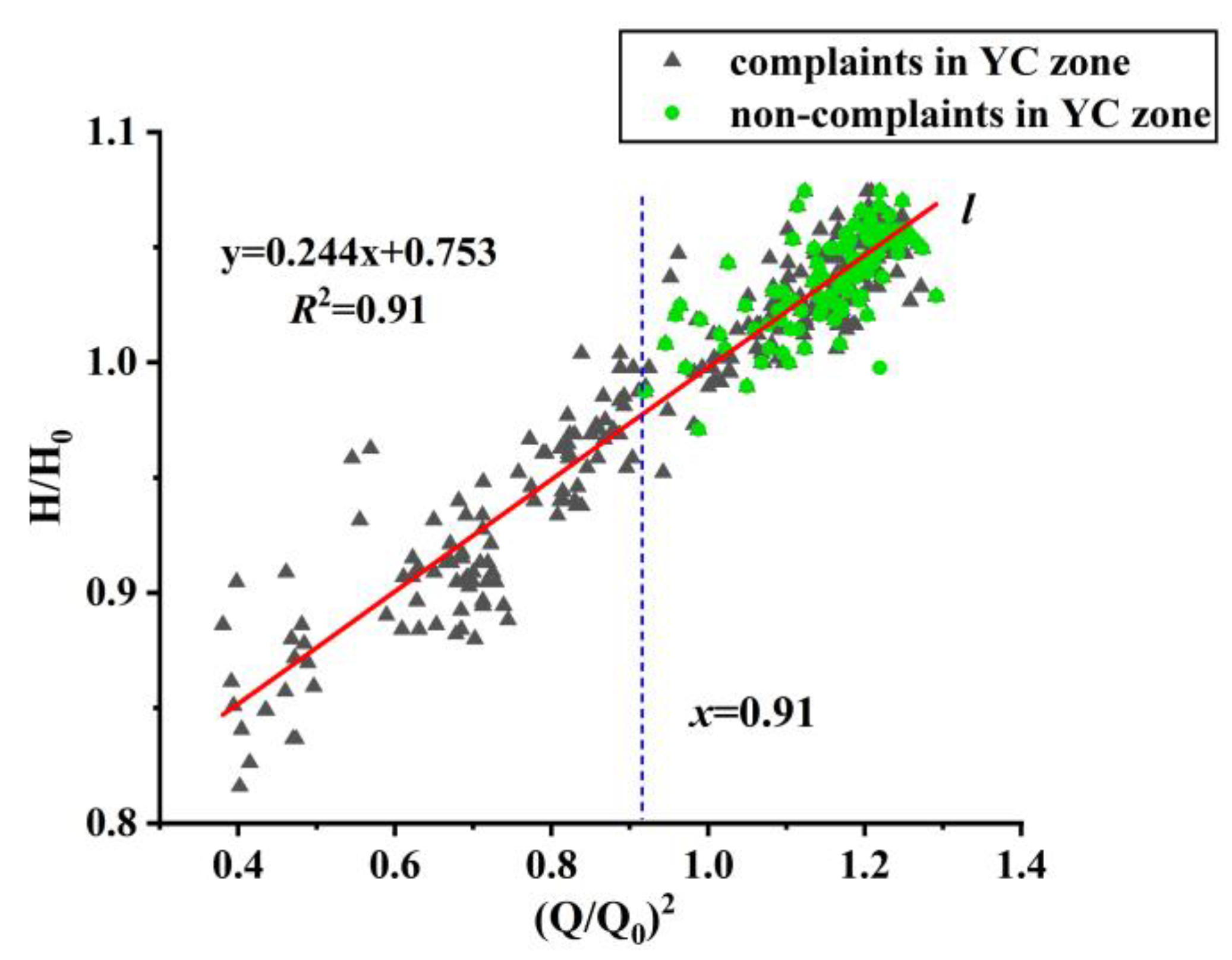
2, as shown in
Figure 6. The data points corresponding to water shortage events are marked in the plot. If one or more water shortages were recorded on a specific day, the corresponding data point was marked with a green circle. Otherwise, it was plotted as a black triangulation point.
In
Figure 6, the black triangulation points represent data for the pressure (
H/H0) and flow rate ((
Q/Q0)
2) at the Xizhou water plant. The green circles indicate water shortages in the YC zone, and the red line represents the fitting line for the black triangulation points. Several patterns can be observed in
Figure 6. (1) The square of the water demand shows a linear relationship with the water pressure. (2) A lower-bound flow rate was observed before the occurrence of shortage events, approximately 95% of the annual average flow rate. This is indicated by the blue line in
Figure 6.
2.2.2. Methodology of Statistical Characteristics
The pressure-flow rate of the water pump station indicates the supply–demand relationship in the operation and scheduling processes of the pipe network and water pump station. After years of adjustment, the scheduling of the water plant and the customer demand pressure reached a dynamic equilibrium. For energy-saving purposes, the water supply pressure was adjusted by the water company based on the number of water shortage records within an acceptable range (for example, no more than 20–30 water shortage complaints per day for the entire GZ city). Under this condition, the following assumptions were proposed.
There exists a critical pressure range at which customers begin to complain about water shortages. When the water pressure satisfies the requirements of water facilities, the probability of a water shortage is low. When the pressure is lower than that in water facilities, customers complain based on the service pressure.
When the water demand exceeds the critical flow rate, the water pump station increases the pressure to improve customers’ experience and minimize complaints. The water company adjusts the water supply pressure within a reasonable range to maintain the balance between economic costs and customers’ complaints.
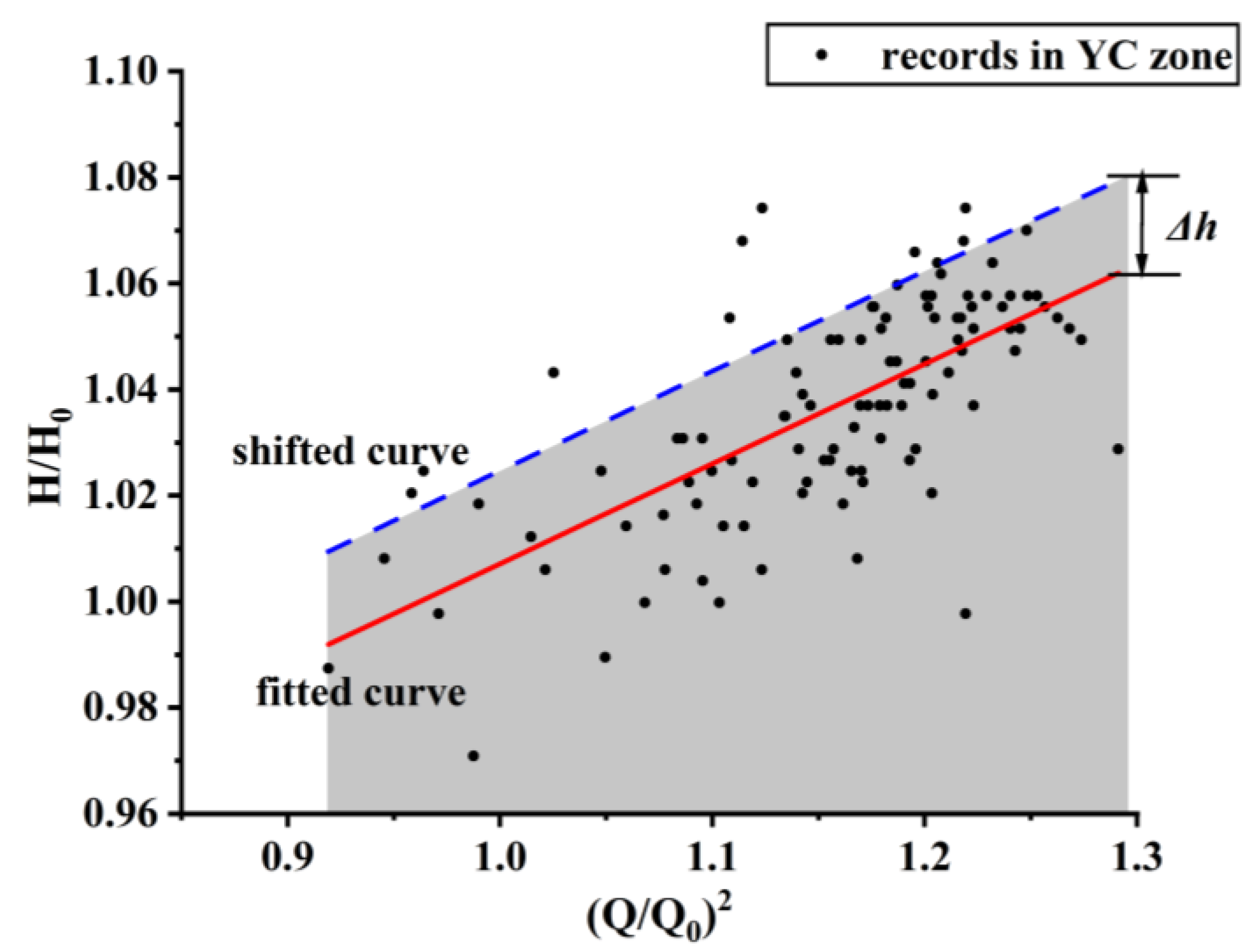
The critical state line of the pressure-flow rate was obtained by fitting the water shortage data points; this line represents the mathematical expectation of the critical water pressure and water demand (
Figure 7).
Equation (5) is used to calculate the water shortage probability under the conditions of specific water demand (
) and pressure change (
). This probability is defined as the ratio of the frequency of water shortage records occurring under the pressure change (
) condition to the sample size, considering the water demand (
) condition. When a specific water demand (
) is provided, there are
samples. Among these samples,
samples experience water shortage when subjected to a pressure change (
). The water shortage probability
under this condition can be denoted as follows:
where
is the number of water shortage records in the water demand (
) when the pressure change (
) alters the critical line, and
is the total number of water shortage records in the water demand (
).
The fitting line of the pressure flow with the water shortage points in
Figure 7 represents the critical value of customer complaints, where the probabilities of complaints and non-complaints are equal. Based on assumption 2, the state of the water pump station is in equilibrium with the customers’ required pressures. Therefore, the probability of water shortage complaints by customers above or below this line is related to the pressure of the water pump station, denoted as
, indicating that the distribution line of the water shortage probability
along the red fitting line in
Figure 7 is similar. The probability of water shortage,
, can be calculated using
. Thus, it is unnecessary to individually count according to
when calculating the probability of a water shortage. The number of water shortage records is counted by shifting
on the fitted line (
Figure 8). This method can reduce the errors caused by insufficient sample sizes.
2.2.3. Water Shortage Distribution Characteristics
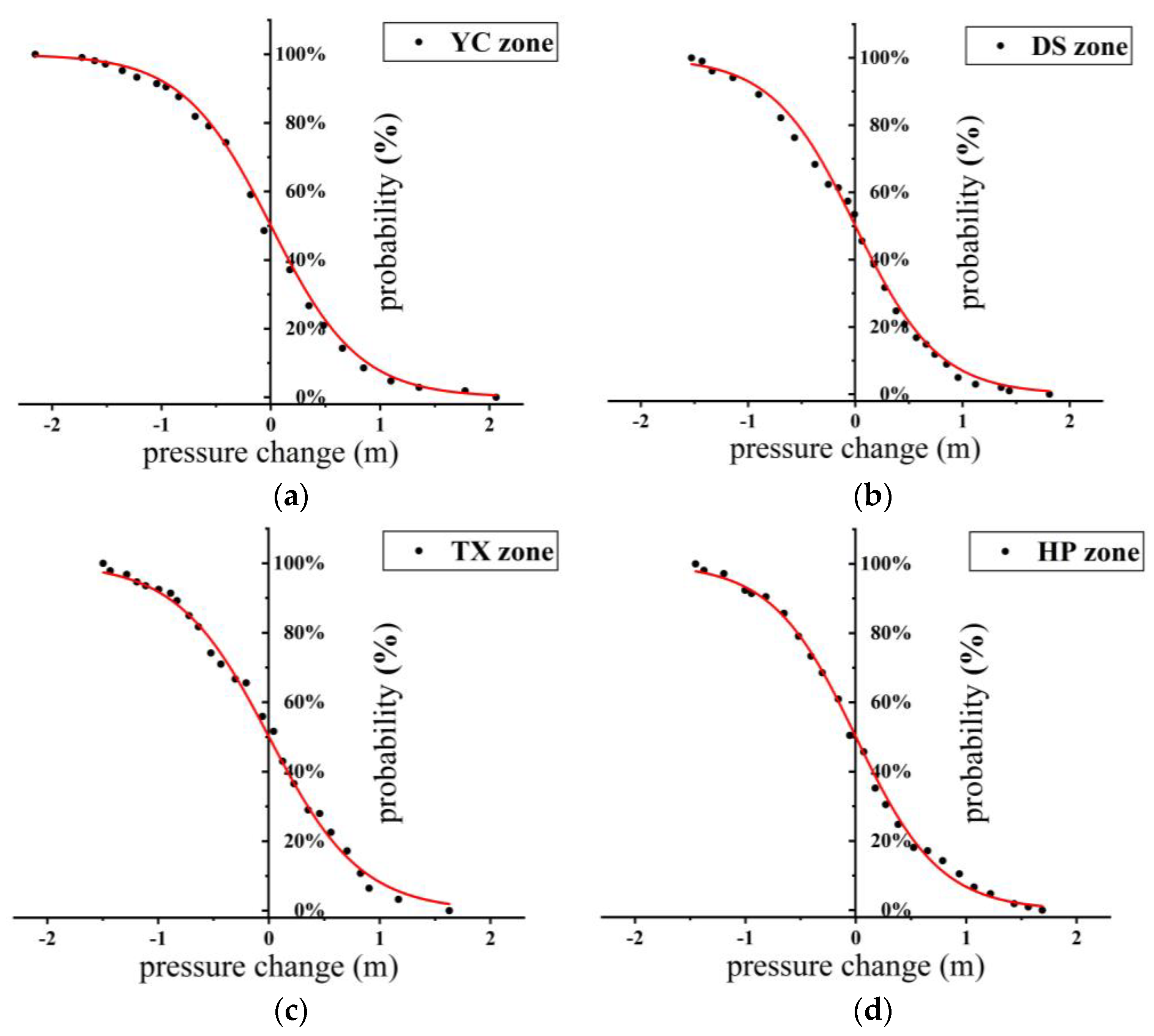
Data from each zone were analyzed for the entire GZ city. The cumulative probability of water shortage records followed the Boltzmann function, as expressed by Equation (6). Parameters Δ
h0 and
A2 in the Boltzmann function were close to zero, whereas
A1 was close to one. By setting the Δ
h0 and
A2 values to 0 and the
A1 value to 1, the activation Sigmoid function widely used in neural networks was obtained, as expressed by Equation (7). The parameters and fitted Sigmoid function lines are presented in
Table 1 and
Figure 9, respectively:
where
,
,
, and
are parameters that must be determined according to the complaint records.
is the shift value of the water head pressure, and
y is the probability of a water shortage in the zone.
3. Results and Discussion
All 59 zones in the GZ city were analyzed. The mean value of was 0.4541 m. The significance level was set at 0.05. The cumulative probability of a water shortage in each zone and the fitted Sigmoid function showed the coefficient of determination, , exceeding 0.99. The Pearson correlation coefficients obtained a range from 0.71 to 0.77. is an important parameter of the Sigmoid function, which determines the slope and compression level of the function curve. In the GZ city, the value of determines the impact of changes in water pressure on customers’ water consumption experience. By understanding and utilizing the value of , policymakers and operators can make informed decisions to optimize water supply management and ensure an enhanced water consumption experience for customers.
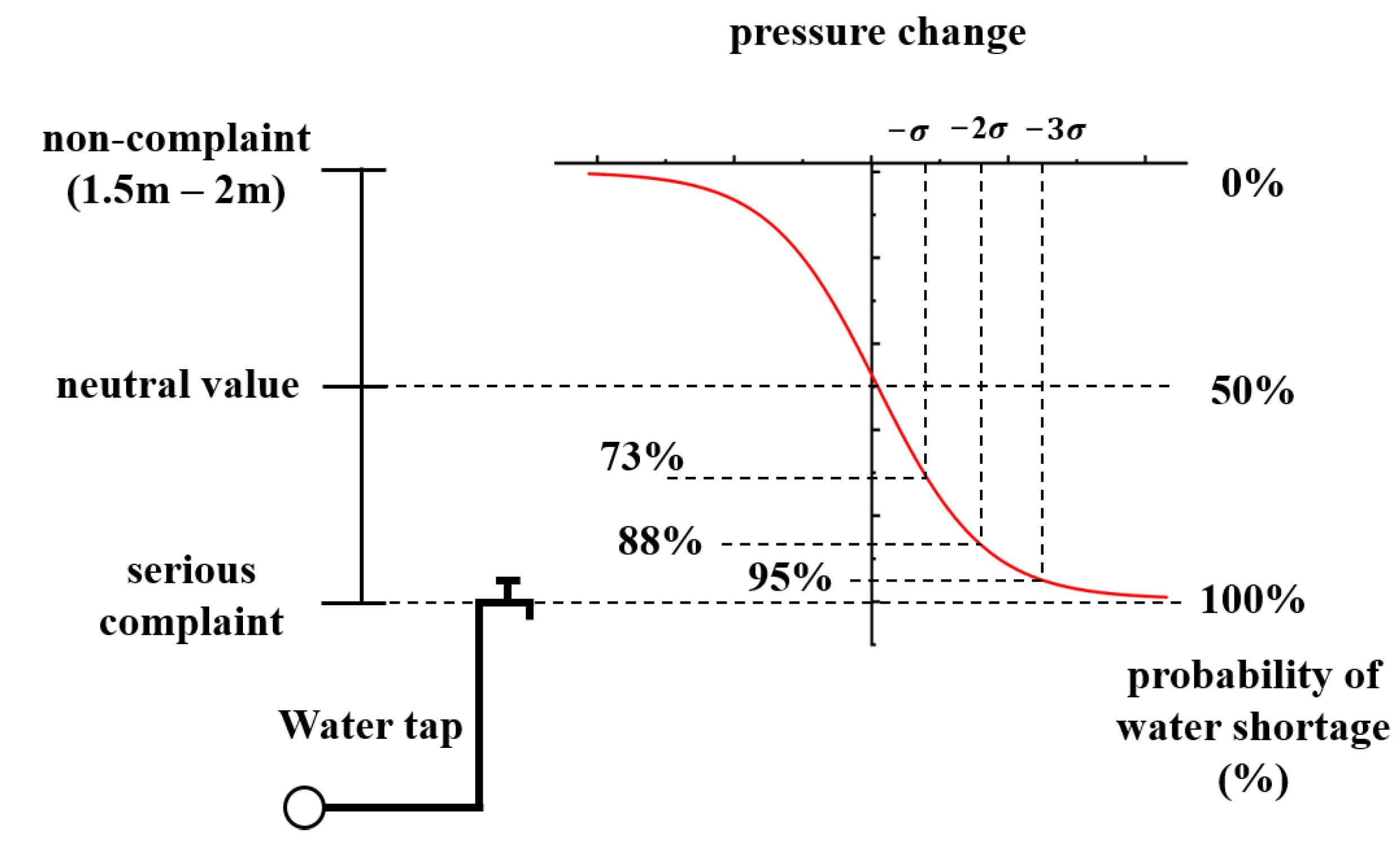
The value of was approximately 0.4–0.5 m. A pressure change, , from to is equivalent to a pressure variation of 1.6–2 m. In China, the required service pressure for water facilities, such as water taps, is generally 15–20 kPa (equivalent to a required water head of 1.5–2 m).
As depicted in
Figure 10, when the water pressure meets the regulatory requirements (water head of 1.5–2 m), customers do not experience water shortages and remain satisfied without raising any complaints. When the water pressure aligns with the water outlet level of the tap, customers experience substantial water shortages, leading to complaints. When the water pressure assumes a neutral value, the probability of customers reporting water shortages becomes equal to the probability of customers not complaining about such issues.
By substituting the water pressure variations, , of , −2, and −3 into Equation (7), the corresponding probabilities of a water shortage can be calculated. This analysis reveals that as a customer’s water pressure changes from a sufficient level to a proximity of −, the probability of reporting a water shortage increases to 73%. When the water pressure changes from sufficient to close to −2, the probability of reporting a water shortage rises to 88%. When the water pressure changes from sufficient to close to −3, the probability of reporting a water shortage escalates to 95%.
Under normal operating conditions, water plants typically maintain the water pressure at the neutral value. At this stage, the service pressure decreases to approximately 50% of the design pressure, and the water discharge from the tap reaches approximately 70% of the design value. This water pressure state serves as a critical value when customers begin to feel that the water supply is insufficient.
The parameters of the statistical model show a close correlation with the physical phenomena. The Sigmoid function is a commonly used mathematical function that is often employed to map inputs to the range [0, 1]. It is interpreted as a probability value, representing the likelihood of an event occurring. The Sigmoid function plays a significant role in machine learning and neural networks, where it is frequently utilized as an activation function. The Sigmoid function describes the reaction of the human nervous system to external stimuli. This relationship is illustrated in
Figure 11, which verifies the rationality of the proposed hypotheses from another perspective.
While satisfying customers’ water demand, the water company will attempt to reduce its energy consumption as much as possible. The water service pressure at the water pump station and the customer demand reached a dynamic balance after long-term operation. The critical water service pressure can be determined by analyzing the water shortage records. Based on the proposed probability model, the possibility of complaints under different water demands and service pressures can be predicted. This can help the water pump station provide water under an economical service pressure.
4. Research Limitations and Suggestions for Further Research
4.1. Research Limitations
The research conducted in this study is specifically applicable to certain regions, such as those with pronounced water scarcity characteristics. As shown in
Figure 6, a water shortage in GZ is characterized by a critical flow threshold, with water shortage events occurring when the ratio (
Q/
Q0)
2 > 0.91 (approximately 95% of the annual average flow). Obtaining data for such specific regions to analyze is not easy because most cities do not experience water scarcity to the extent that the GZ city does. Therefore, not every city can undertake similar studies.
4.2. Suggestions for Further Research
Based on the statistical features derived from the data, this study has revealed specific physical implications that can serve as a reference for regulating the operation of urban water supply and guiding the transformation of water distribution networks. In light of these findings, future research can be expanded in the following two areas:
Reference for operational adjustments of water distribution systems: When a certain number of water shortage events occur, water pump adjustments are required. Water companies can adjust their service pressures based on the water shortage probability function.
Water distribution system construction: If a new pipeline is constructed in a water supply system, the local pressure in the pipeline network increases. Based on the hydraulic model of the pipeline network, the improvement of pressure can be calculated, and a statistical model can be used to estimate the reduction in water shortage probability. The model can also be used to predict the critical water demand during water shortages after a pipeline is constructed.
5. Conclusions
Water shortage records serve as feedback and monitoring methods for water supply systems, reflecting whether the system satisfies the requirements of water pressure from customers. This study analyzed the characteristics of water shortage records in a real-life pipe system and established a statistical model.
The heat map can visualize the data of the water shortage records and help determine the spatial location and intensity of water shortages. However, it cannot inform water companies when a water shortage occurs or state how much improvement in water service pressure can reduce customer complaints.
To satisfy customer requirements, the water company adjusts the pressure according to water demand. The service pressure (H) and water demand (Q2) of the water pump station exhibit a linear relationship. Water shortage events are related to the water demand. Customers complain when the water demand exceeds the critical values of different zones. The critical pressure line for water shortage can be fitted to water shortage samples. The cumulative probability of the samples indicates that water shortage events follow the pattern of the artificial neural function. The critical parameters of the model reflected the requirements for water facility service pressures.
This study proposes a novel method to help water companies analyze fuzzy water shortage records using a quantitative model. The proposed method can be used to determine the effects of pressure adjustments and pipeline construction on customer requirements.
Author Contributions
Conceptualization, W.C. and H.L.; methodology, W.C. and H.L.; software, W.C.; validation, Z.L. and G.X.; formal analysis, W.C.; investigation, L.T.; resources, Z.L. and G.X.; data curation, Z.L., G.X. and L.T.; writing—original draft preparation, H.L.; writing—review and editing, W.C.; visualization, H.L.; supervision, W.C.; project administration, W.C.; funding acquisition, W.C. All authors have read and agreed to the published version of the manuscript.
Funding
This research was funded by the Science and Technology Plan Project of the Ministry of Housing and Urban-Rural Development, grant number 2022-K-161, the Zhejiang Province Key Research and Development Program Project, grant number 2021C03017, and the Guangzhou Water Supply Company, grant number Science and Technology 21-2.
Data Availability Statement
Please contact the corresponding author for data.
Conflicts of Interest
The authors declare no conflict of interest.
References
- Mortula, M.M.; Ali, T.A.; Sadiq, R.; Idris, A.; Al Mulla, A. Impacts of Water Quality on the Spatiotemporal Susceptibility of Water Distribution Systems. Clean–Soil Air Water 2019, 47, 1800247. [Google Scholar] [CrossRef]
- Cabrera, E.; Gómez, E.; Cabrera, E.; Soriano, J.; Espert, V. Energy Assessment of Pressurized Water Systems. J. Water Resour. Plann. Manag. 2015, 141, 04014095. [Google Scholar] [CrossRef]
- Hashemi, S.; Filion, Y.R.; Speight, V.L. Pipe-Level Energy Metrics for Energy Assessment in Water Distribution Networks. Procedia Eng. 2015, 119, 139–147. [Google Scholar] [CrossRef]
- Cabrera, E.; Cabrera, E.; Cobacho, R.; Soriano, J. Towards an Energy Labelling of Pressurized Water Networks. Procedia Eng. 2014, 70, 209–217. [Google Scholar] [CrossRef]
- Goel, D.; Chaudhury, S.; Ghosh, H. Smart Water Management: An Ontology-Driven Context-Aware IoT Application. In Pattern Recognition and Machine Intelligence; Shankar, B.U., Ghosh, K., Mandal, D.P., Ray, S.S., Zhang, D., Pal, S.K., Eds.; Lecture Notes in Computer Science; Springer International Publishing: Cham, Switzerland, 2017; Volume 10597, pp. 639–646. [Google Scholar] [CrossRef]
- Jeong, G.; Wicaksono, A.; Kang, D. Revisiting the Resilience Index for Water Distribution Networks. J. Water Resour. Plan. Manag. 2017, 143, 04017035. [Google Scholar] [CrossRef]
- Atkinson, S.; Farmani, R.; Memon, F.A.; Butler, D. Reliability Indicators for Water Distribution System Design: Comparison. J. Water Resour. Plan. Manag. 2014, 140, 160–168. [Google Scholar] [CrossRef]
- Greco, R.; Di Nardo, A.; Santonastaso, G. Resilience and Entropy as Indices of Robustness of Water Distribution Networks. J. Hydroinform. 2012, 14, 761–771. [Google Scholar] [CrossRef]
- Raad, D.N.; Sinske, A.N.; van Vuuren, J.H. Comparison of Four Reliability Surrogate Measures for Water Distribution Systems Design: Comparison of WDS Reliability Surrogates. Water Resour. Res. 2010, 46, W05524. [Google Scholar] [CrossRef]
- Jun, H.; Loganathan, G.V.; Kim, J.H.; Park, S. Identifying Pipes and Valves of High Importance for Efficient Operation and Maintenance of Water Distribution Systems. Water Resour. Manag. 2008, 22, 719–736. [Google Scholar] [CrossRef]
- Jayaram, N.; Srinivasan, K. Performance-Based Optimal Design and Rehabilitation of Water Distribution Networks Using Life Cycle Costing: WATER DISTRIBIUTION NETWORKS. Water Resour. Res. 2008, 44. [Google Scholar] [CrossRef]
- Khomsi, D.; Walters, G.A.; Thorley, A.R.D.; Ouazar, D. Reliability Tester for Water-Distribution Networks. J. Comput. Civ. Eng. 1996, 10, 10–19. [Google Scholar] [CrossRef]
- Kim, S.; Jeong, S.; Woo, I.; Jang, Y.; Maciejewski, R.; Ebert, D.S. Data Flow Analysis and Visualization for Spatiotemporal Statistical Data without Trajectory Information. IEEE Trans. Visual. Comput. Graph. 2018, 24, 1287–1300. [Google Scholar] [CrossRef] [PubMed]
- Fobil, J.N.; Levers, C.; Lakes, T.; Loag, W.; Kraemer, A.; May, J. Mapping Urban Malaria and Diarrhea Mortality in Accra, Ghana: Evidence of Vulnerabilities and Implications for Urban Health Policy. J. Urban Health 2012, 89, 977–991. [Google Scholar] [CrossRef] [PubMed]
- Osei, F.B.; Stein, A. Spatial Variation and Hot-Spots of District Level Diarrhea Incidences in Ghana: 2010–2014. BMC Public Health 2017, 17, 617. [Google Scholar] [CrossRef] [PubMed]
- Huang, H.; Yang, H.; Chen, Y.; Chen, T.; Bai, L.; Peng, Z.-R. Urban Green Space Optimization Based on a Climate Health Risk Appraisal–A Case Study of Beijing City, China. Urban For. Urban Green. 2021, 62, 127154. [Google Scholar] [CrossRef]
- Khalid, S.; Shoaib, F.; Qian, T.; Rui, Y.; Bari, A.I.; Sajjad, M.; Shakeel, M.; Wang, J. Network Constrained Spatio-Temporal Hotspot Mapping of Crimes in Faisalabad. Appl. Spat. Anal. 2018, 11, 599–622. [Google Scholar] [CrossRef]
- Wang, D.; Ding, W.; Lo, H.; Morabito, M.; Chen, P.; Salazar, J.; Stepinski, T. Understanding the Spatial Distribution of Crime Based on Its Related Variables Using Geospatial Discriminative Patterns. Comput. Environ. Urban Syst. 2013, 39, 93–106. [Google Scholar] [CrossRef]
- Mao, Y.; Qin, G.; Ni, P.; Liu, Q. Analysis of Road Traffic Speed in Kunming Plateau Mountains: A Fusion PSO-LSTM Algorithm. Int. J. Urban Sci. 2022, 26, 87–107. [Google Scholar] [CrossRef]
- Tang, J.; Wang, X.; Zong, F.; Hu, Z. Uncovering Spatio-Temporal Travel Patterns Using a Tensor-Based Model from Metro Smart Card Data in Shenzhen, China. Sustainability 2020, 12, 1475. [Google Scholar] [CrossRef]
- Shao, H.; Sun, H.; Cui, W. Chinese Word Segmentation Based on Improved Double Hashtable. In Proceedings of the Fifth International Conference on Machine Vision (ICMV 2012): Computer Vision, Image Analysis and Processing, Wuhan, China, 13 March 2013; Wang, Y., Tan, L., Zhou, J., Eds.; SPIE: Bellingham, WA, USA, 2013; p. 87830U. [Google Scholar] [CrossRef]
- Xiong, Z. An Algorithm Rapidly Segmenting Chinese Sentences into Individual Words. MATEC Web Conf. 2019, 267, 04001. [Google Scholar] [CrossRef]
- Liu, Z.; Zheng, T.; Xu, G.; Yang, Z.; Liu, H.; Cai, D. Training-Time-Friendly Network for Real-Time Object Detection. arXiv 2019, arXiv:1909.00700. [Google Scholar] [CrossRef]
- Schoier, G.; Borruso, G. Spatial Data Mining for Highlighting Hotspots in Personal Navigation Routes. Int. J. Data Warehous. Min. 2012, 8, 45–61. [Google Scholar] [CrossRef]
- Škuta, C.; Bartůněk, P.; Svozil, D. InCHlib–Interactive Cluster Heatmap for Web Applications. J. Cheminform. 2014, 6, 44. [Google Scholar] [CrossRef] [PubMed]
- Huang, C.-W.; Shih, T.-Y. On the Complexity of Point-in-Polygon Algorithms. Comput. Geosci. 1997, 23, 109–118. [Google Scholar] [CrossRef]
- García Zapata, J.-L.; Díaz Martín, J.C. A Geometric Algorithm for Winding Number Computation with Complexity Analysis. J. Complex. 2012, 28, 320–345. [Google Scholar] [CrossRef]
- Hormann, K.; Agathos, A. The Point in Polygon Problem for Arbitrary Polygons. Comput. Geom. 2001, 20, 131–144. [Google Scholar] [CrossRef]
- Ochilbek, R. A New Approach (Extra Vertex) and Generalization of Shoelace Algorithm Usage in Convex Polygon (Point-in-Polygon). In Proceedings of the 2018 14th International Conference on Electronics Computer and Computation (ICECCO), Kaskelen, Kazakhstan, 29 November–1 December 2018; pp. 206–212. [Google Scholar] [CrossRef]
- Fu, Q.; Liang, X.; Zhang, J.; Qi, D.; Zhang, X. A Geofence Algorithm for Autonomous Flight Unmanned Aircraft System. In Proceedings of the 2019 International Conference on Communications, Information System and Computer Engineering (CISCE), Haikou, China, 5–7 July 2019; pp. 65–69. [Google Scholar] [CrossRef]
| Disclaimer/Publisher’s Note: The statements, opinions and data contained in all publications are solely those of the individual author(s) and contributor(s) and not of MDPI and/or the editor(s). MDPI and/or the editor(s) disclaim responsibility for any injury to people or property resulting from any ideas, methods, instructions or products referred to in the content. |
© 2023 by the authors. Licensee MDPI, Basel, Switzerland. This article is an open access article distributed under the terms and conditions of the Creative Commons Attribution (CC BY) license (https://creativecommons.org/licenses/by/4.0/).
