Study on Numerical Modeling for Pollutants Movement Based on the Wave Parabolic Mild Slope Equation in Curvilinear Coordinates

Abstract

Nearshore waves and currents induced by breaking of obliquely incident waves are important dynamic factors that significantly affect pollutants movement at offshore zones. A combined numerical model in orthogonal curvilinear coordinates is developed to simulate pollutants movement in surf zones, including a wave transformation model based on the parabolic mild slope equation, a wave-induced current model, and a pollutant transport model driven by waves and currents. This combined model has been applied to pollutants movement laboratory cases, and comparison of the simulations with experimental measurements shows good agreement. The model has also been applied to simulation of the Gourlay experiment and it shows consistent results with the distribution of waves and offshore currents. This coupled numerical model has preliminarily improved the situation of rare numerical research on the nearshore pollutant transport in coastal wave and wave-induced current based on wave radiation stress theory in orthogonal curvilinear coordinates.

1. Introduction

With increasingly frequent human activities in the coastal waters, large amounts of industrial and domestic wastewater are discharged into coastal waters. This seriously pollutes coastal waters and significantly decreases the quality of the coastal water ecological environment. This offshore environmental pollution problem is increasingly prominent. Maintaining the health and sustainability of the offshore environment has attracted significant attention from governments and environmental organizations [1]. In order to manage and protect the nearshore seawater ecological environment and provide a good environment for the development and construction of coastal areas, it is an effective means to analyze and reveal the movement regulation of discharged pollutants under the action of nearshore seawater dynamic factors based on the distribution regulation of nearshore hydrodynamic factors.

The nearshore sea is one of the most complex areas in terms of distribution of various environmental dynamic factors, especially in the mild coast, due to the influence of geomorphology and shore boundaries, wave fragmentation, evolution, and other phenomena; the strong nearshore current is formed, making the hydrodynamic structure of the nearshore sea exceptionally complex. Many scholars have conducted numerous studies on the nearshore wave-current system [2,3,4,5,6,7,8,9], and further studies have shown that the transport pattern of pollutants in nearshore waters is closely related to these nearshore hydrodynamic factors [10], and that this transport pattern it is obviously different from the transport of pollutants under the effect of pure current without considering the influence of waves. The effective analysis of wave-current field and pollutant transport regulation at the nearshore mild sloping coast is of great theoretical value and practical significance to the coastal zone environmental protection, ecological planning, and offshore projects implementation.

In the past, the numerical study of pollutant transport based on nearshore wave-current field was mostly solved in the cartesian coordinate system with a discretized format in the rectangular grid system. However, for the complex boundary in actual domain, such as the coast, islands, and offshore buildings, the geometric boundary is often irregular, and the calculation boundary does not match the actual boundary very well during numerical simulation. This does not only reduce the accuracy of the numerical simulation at the physical boundary, but it increases the complexity of boundary conditions setting, thereby producing computational errors. Therefore, since the 1980s, scholars have been studying and developing boundary-applicable curvilinear grid techniques for the numerical simulation of offshore waves and nearshore currents. Kirby et al. [11,12] introduced the concepts of body-fitted coordinate and conformal mapping to the wave mild slope equation in curvilinear coordinates and derived exact expressions for the propagation of regular waves in semicircular curves. Based on the Boussinesq model developed by Kirby and Shi et al. [13], some recent studies about the real applications of their numerical model near the shoreline have been presented [14,15]. These studies show that under the curvilinear coordinate system, the grid layout in the computational domain is flexible and adaptive to the irregular boundary. The curvilinear grids fit completely on the physical boundaries, making the processing of boundary conditions simple and greatly improving the computational accuracy. In the research area of nearshore pollutant transport, several researchers [16,17] have made progress on both mechanism and numerical modeling and have gradually revealed the characteristics of nearshore pollutant transport; this achievement, however, is mostly limited to the cartesian coordinate system or regular region. Although the numerical study of nearshore wave propagation based on the mild slope equation or the Boussinesq equation in the curved coordinate system is becoming mature, the intensive study of nearshore wave-current fields based on the wave radiation stress theory combined with the mild slope equation in curved coordinate system is still rare, and the further coupled numerical model of pollutant with wave-current fields in curved coordinate system to simulate the nearshore pollutant transport is even rarer.

In this paper, based on the principle of orthogonal curve transformation, a combined numerical model in orthogonal curvilinear coordinates is developed to simulate pollutants transport in breaking waves-induced offshore currents in surf zones with curved boundary or irregular coastlines, including a wave transformation model based on the parabolic mild slope equation, a wave-induced offshore current model, and a pollutant transport model. The numerical results of this combined model have been verified and analyzed by the data of experiments conducted at the State Key Laboratory of Coastal and Offshore Engineering of Dalian University of Technology on the transport of pollutants under the co-action of waves and currents. Furthermore, the combined numerical model has been applied to the Gourlay experiment on pollutants transport with complex boundaries and topographic conditions, and the simulated results of pollutants transport consist with the distribution of waves and nearshore currents in the case [18]. This coupled numerical model has preliminarily improved the situation of rare numerical research on the nearshore pollutant transport in coastal wave and wave-induced current based on wave radiation stress theory in orthogonal curvilinear coordinates.

2. Methodology

2.1. Numerical Model of Wave Propagation

When the waves propagate into the coastal zone, the waves will be deformed and broken due to the shallow topography, and nearshore currents induced by breaking of obliquely incident waves are formed. The calculation of wave propagation is determinate to nearshore currents modeling. In order to overcome the problem of complex vector curvilinear parabolic approximation, the wave-current interaction governing equation proposed by Kirby [19] applied the covariance-inversion tensor method to propose a curvilinear parabolic gentle slope equation, which is suitable for numerical simulation of wave propagation in orthogonal curvilinear coordinate system. This is achieved by neglecting the currents velocity vector, the less influential term, and the non-orthogonal term in the equation. The parabolic mild slope equation can be obtained in the following form:

$$\begin{array}{l}\sqrt{g^{11}}{C}_g{A}_{\xi }-\frac{\mathrm{i}}{2\omega }\frac{p}{J}{J}_{\eta }{g}^{22}{A}_{\eta }+(\mathrm{i}(\overline{k^{\prime }}-k^{\prime })\sqrt{g^{11}}{C}_g+\frac{1}{2}(\sqrt{g^{11}}{C}_g{)}_{\xi }+\frac{\mathrm{i}}{2}\omega k^{\prime }{}^2{g}^{11}D\left|A\right|\\ +\frac{D_b}{2}+\frac{\overline{k^{\prime }}}{2\omega }\frac{p}{J}{J}_{\xi }{g}^{11})A+(\frac{\beta }{4\omega }-\frac{\mathrm{i}}{2\omega })(g^{22}p{A}_{\eta }{)}_{\eta }+\frac{1}{4k^{\prime }\omega }(g^{22}p{A}_{\eta }{)}_{\eta \xi }=0\end{array}$$

(1)

$$g^{11}=(\raisebox{1ex}{$g_{\eta }$}\!\left/ \!\raisebox{-1ex}{$J$}\right.{)}^2$$

$$g^{22}=(\raisebox{1ex}{$g_{\xi }$}\!\left/ \!\raisebox{-1ex}{$J$}\right.{)}^2$$

$$D=k^3\frac{C}{C_g}\frac{(\cosh (4kh)+8-2{\tanh }^2(kh))}{8{\sinh }^4(kh)}$$

$$D_b=\frac{K{C}_g}{h}(1-\raisebox{1ex}{$E_s$}\!\left/ \!\raisebox{-1ex}{$E$}\right.)$$

$$k^{\prime }=\raisebox{1ex}{$k$}\!\left/ \!\raisebox{-1ex}{$\sqrt{g^{11}}$}\right.$$

$$\overline{k^{\prime }}=\frac{1}{{\eta }_2-{\eta }_1}{\displaystyle \int {}_{{\eta }_1}^{{\eta }_2}}{k}^{\prime }(\xi ,\eta )d\eta$$

$$\beta =\raisebox{1ex}{$k_{\xi }^{\prime }$}\!\left/ \!\raisebox{-1ex}{$k^{\prime }{}^2$}\right.+\raisebox{1ex}{$(k^{\prime }{g}^{11}p{)}_{\xi }$}\!\left/ \!\raisebox{-1ex}{$2k^{\prime }{}^2{g}^{11}p$}\right.$$

where, i is an imaginary unit; J is the Jacobian coefficient; A is the spatially varying wave complex amplitude; ω is the wave angular frequency; k is the local wave number; C is the wave propagation phase velocity; C_g is the wave propagation group velocity; p = CC_g; h is the local water depth; r is the density of seawater; g is the acceleration of gravity; E = ρgh²/8, is the wave energy; E_s is the wave energy where the wave height is stable after wave breaking [20]; D is the factor considering the nonlinear effect of waves; D_b is the energy loss rate of wave breaking; K ≈ 0.15 is the empirical coefficient. ξ and η are independent variables in the transformed image domain; and g_ξ and g_η are Lame coefficients.

In surf zones, it is often considered that the wave breaks at a point when the wave height H is greater than the maximum breaking height Hb at that point. In shallow water, H_b can be determined by the following equation [21].

$$H_b=\min (\gamma h,0.14L\tanh kh)$$

(2)

where, γ is the ratio parameter for guiding the breaking waves, and it ranges from 0.6 to 0.8 according to local topography; L is the wave length.

For a given incident wave amplitude A₀, wave number k₀ and wave incident angle in the cartesian coordinate system with respect to the main wave propagation direction a₀ at the boundary, the wave incident boundary can be set as,

$$A=A_0{e}^{i\int (x_{\eta }{k}_0\cos {\alpha }_0+y_{\eta }{k}_0\sin {\alpha }_0)d\eta }$$

(3)

For the side boundary conditions, Zhang et al. [22] proposed an expression that unified the open boundary and the solid boundary with different reflection properties.

$$\frac{\partial A}{\partial n}+\phi A=0$$

(4)

where, n is the outer normal direction of the boundary,

$$\phi ={\phi }_r+i{\phi }_i=ik\sin (\theta -\delta )\frac{1-R}{1+R}$$

$${\phi }_r=k\sin (\theta -\delta )\frac{2R_r\sin {\epsilon }_r}{1+R_r^2+2R_r\cos {\epsilon }_r}$$

$${\phi }_i=k\sin (\theta -\delta )\frac{1-R_r^2}{1+R_r^2+2R_r\cos {\epsilon }_r}$$

where, θ is the wave direction angle of the interface; δ is the tangential direction angle of the boundary; $R=R_r{e}^{i{E}_r}$, is the complex reflection coefficient; R_r is the reflection coefficient; and ε_r is the phase difference. For a fully reflective boundary, the reflection coefficient is taken as 1, and Equation (4) is transformed into

$$\frac{\partial A}{\partial n}=0$$

(5)

For the complete radiation boundary, the reflection coefficient is taken to be 0, thus Equation (4) is transformed into

$$\frac{\partial A}{\partial n}+ik\sin (\theta -\delta )A=0$$

(6)

Numerical discretization of the side boundary conditions in the curved coordinate system, the left side boundary along the wave propagation direction takes the form,

$$-\frac{\partial A}{\partial \xi }(\frac{y_{\eta }\sin {\delta }_1+x_{\eta }\cos {\delta }_1}{J})+\frac{\partial A}{\partial \eta }(\frac{y_{\xi }\sin {\delta }_1+x_{\xi }\cos {\delta }_1}{J})+\phi A=0$$

(7)

and the right side boundary along the wave propagation direction takes the form,

$$\frac{\partial A}{\partial \xi }(\frac{y_{\eta }\sin {\delta }_2+x_{\eta }\cos {\delta }_2}{J})-\frac{\partial A}{\partial \eta }(\frac{y_{\xi }\sin {\delta }_2+x_{\xi }\cos {\delta }_2}{J})+\phi A=0$$

(8)

where, δ₁ is the left boundary tangent direction angle and δ₂ is the right boundary tangent direction angle.

2.2. Numerical Model of Nearshore Currents

The wave action on nearshore currents mainly derives from the wave radiation stress. The orthogonal transformation of the depth-averaged two-dimensional shallow water equations in the cartesian coordinate system leads to the following governing equations for the nearshore current fields in the orthogonal curved coordinate system,

$$\frac{\partial z}{\partial t}+\frac{1}{g_{\xi }{g}_{\eta }}\frac{\partial }{\partial \xi }\left(\left(h+z\right)U{g}_{\eta }\right)+\frac{1}{g_{\xi }{g}_{\eta }}\frac{\partial }{\partial \eta }\left(\left(h+z\right)V{g}_{\xi }\right)=0$$

(9)

$$\frac{\partial U}{\partial t}+\frac{U}{g_{\xi }}\frac{\partial U}{\partial \xi }+\frac{V}{g_{\eta }}\frac{\partial U}{\partial \eta }+\frac{UV}{g_{\xi }{g}_{\eta }}\frac{\partial g_{\xi }}{\partial \eta }-\frac{V^2}{g_{\xi }{g}_{\eta }}\frac{\partial g_{\eta }}{\partial \xi }+\frac{g}{g_{\xi }}\frac{\partial z}{\partial \xi }+F_{s\xi }+\frac{1}{\rho \left(h+z\right)}\left({\tau }_{b\xi }-{\tau }_{\xi }\right)-A_{m\xi }=0$$

(10)

$$\frac{\partial V}{\partial t}+\frac{U}{g_{\xi }}\frac{\partial V}{\partial \xi }+\frac{V}{g_{\eta }}\frac{\partial V}{\partial \eta }+\frac{UV}{g_{\xi }{g}_{\eta }}\frac{\partial g_{\eta }}{\partial \xi }-\frac{U^2}{g_{\xi }{g}_{\eta }}\frac{\partial g_{\xi }}{\partial \eta }+\frac{g}{g_{\eta }}\frac{\partial z}{\partial \eta }+F_{s\eta }+\frac{1}{\rho \left(h+z\right)}\left({\tau }_{b\eta }-{\tau }_{\eta }\right)-A_{m\eta }=0$$

(11)

where, t is time; g is the acceleration of gravity; U and V are the currents velocity components averaged along the water depth in the ξ and η directions, respectively; z is the mean water surface; h is the water depth; F_Sξ and F_Sη are the wave radiation stress terms in the ξ and η directions, respectively; τ_ξ and τ_η are the surface shear stress components in the ξ and η directions, respectively; τ_bξ and τ_bη are the bottom shear stress components in the wave-current fields in the ξ and η directions, respectively; A_mξ and A_mη are the lateral turbulent stress terms in the ξ and η directions, respectively.

For the wave radiation stress term in the orthogonal curve coordinate system can be treated as follows,

$$F_{S\xi }=\frac{1}{\rho (h+z)}(\frac{\partial S_{\xi \xi }}{g_{\xi }\partial \xi }+\frac{\partial S_{\xi \eta }}{g_{\eta }\partial \eta })$$

(12)

$$F_{S\eta }=\frac{1}{\rho (h+z)}(\frac{\partial S_{\eta \xi }}{g_{\xi }\partial \xi }+\frac{\partial S_{\eta \eta }}{g_{\eta }\partial \eta })$$

(13)

where S_ξξ, S_ξη, S_ηξ and S_ηη are the wave radiation stress components in the orthogonal curve coordinate system, respectively, and the expressions [23] are

$$S_{\xi \xi }=\frac{\rho g{H}^2}{8}((2\frac{C_g}{C}-\frac{1}{2})-\frac{C_g}{C}{\sin }^2\theta )$$

(14)

$$S_{\xi \eta }=S_{\eta \xi }=\frac{\rho g{H}^2}{8}\frac{C_g}{C}\sin \theta \cos \theta$$

(15)

$$S_{\eta \eta }=\frac{\rho g{H}^2}{8}((\frac{C_g}{C}-\frac{1}{2})+\frac{C_g}{C}{\sin }^2\theta )$$

(16)

where, H is the wave height and θ is the wave direction angle.

The bottom shear stress distribution in the wave-current fields is quite complex, and many scholars have conducted a lot of research work on it, but the calculation formulas are significantly different. In this paper, the following equation [24] is used for the bottom shear stress,

$${\tau }_{b\xi }=\frac{4}{\pi }\rho c_f{u}_{0}U$$

(17)

$${\tau }_{b\eta }=\frac{2}{\pi }\rho c_f{u}_{0}V$$

(18)

where, u₀ = 2πa₀/T derived from the linear wave theory is the horizontal velocity of bottom wave water quality point; T is the wave period; a₀ = H/(2sinhkh) is the horizontal trajectory amplitude of bottom wave water quality point; and c_f for the bottom friction coefficient under the combined effect of current.

The lateral turbulent stress plays an important role in influencing the flow velocity distribution in surf zone, which can be defined by the following equation.

$$A_{m\xi }=\frac{1}{g_{\xi }{g}_{\eta }}(\frac{\partial }{\partial \xi }(g_{\eta }{\sigma }_{\xi \xi })+\frac{\partial }{\partial \eta }(g_{\xi }{\sigma }_{\eta \xi })+{\sigma }_{\xi \eta }\frac{\partial g_{\xi }}{\partial \eta }-{\sigma }_{\eta \eta }\frac{\partial g_{\eta }}{\partial \xi })$$

(19)

$$A_{m\eta }=\frac{1}{g_{\xi }{g}_{\eta }}(\frac{\partial }{\partial \xi }(g_{\eta }{\sigma }_{\xi \eta })+\frac{\partial }{\partial \eta }(g_{\xi }{\sigma }_{\eta \eta })+{\sigma }_{\eta \xi }\frac{\partial g_{\eta }}{\partial \xi }-{\sigma }_{\xi \xi }\frac{\partial g_{\xi }}{\partial \eta })$$

(20)

where, σ_ξξ, σ_ξη, σ_ηξ, σ_ηη are the lateral turbulent stress components.

$${\sigma }_{\xi \xi }=2\mu (\frac{1}{g_{\xi }}\frac{\partial U}{\partial \xi }+\frac{V}{g_{\xi }{g}_{\eta }}\frac{\partial g_{\xi }}{\partial \eta })$$

(21)

$${\sigma }_{\eta \eta }=2\mu (\frac{1}{g_{\eta }}\frac{\partial V}{\partial \xi }+\frac{UV}{g_{\xi }{g}_{\eta }}\frac{\partial g_{\eta }}{\partial \xi })$$

(22)

$${\sigma }_{\xi \eta }={\sigma }_{\eta \xi }=\mu (\frac{g_{\eta }}{g_{\xi }}\frac{\partial }{\partial \xi }(\frac{V}{g_{\eta }})+\frac{g_{\xi }}{g_{\eta }}\frac{\partial }{\partial \eta }(\frac{U}{g_{\xi }}))$$

(23)

where, μ is the lateral turbulence admixture coefficient under wave action, and the expression for μ given in this paper using the L-H model [25] is as follows,

$$\mu =N{x}_l\sqrt{gh}$$

(24)

where, x_l is the shore distance of the wave breaking point and N is the uncaused quantity. Outside the breaking zone, μ is usually taken as a constant, and its value is the value at the wave breaking point.

The governing Equations (9)–(11) of the numerical model of the nearshore wav-current fields are non-constant systems equations, so the required fixed solution conditions include the initial conditions and the boundary conditions of the computational domain. In the calculation, the initial conditions can be set to $U=0$, $V=0$, $\frac{\partial z}{\partial \mathrm{n}}=0$, where n is the outer normal direction of the boundary; for the outer sea boundary away from the wave breaking area, only considering the currents induced by waves, the approximation is $U=0$, $V=0$, $z=0$; for the open side of the boundary with relatively mild topographic changes, set to $\frac{\partial U}{\partial \mathrm{n}}=0$, $\frac{\partial V}{\partial \mathrm{n}}=0$, $\frac{\partial \mathrm{z}}{\partial \mathrm{n}}=0$.

2.3. Numerical Model of Nearshore Pollutant Transport under Co-Action of Waves and Currents

The depth-averaged pollutant transport equation in the orthogonal curve coordinate system can be derived by the orthogonal transformation from its formula in the cartesian coordinate system as follows,

$$\begin{array}{l}\frac{\partial c}{\partial t}+\frac{U}{g_{\xi }{g}_{\eta }}\frac{\partial c}{\partial \xi }+\frac{V}{g_{\xi }{g}_{\eta }}\frac{\partial c}{\partial \eta }=\\ \frac{1}{H{g}_{\xi }{g}_{\eta }}[\frac{\partial }{\partial \xi }(H{\Gamma }_{cw\xi }\frac{g_{\eta }}{g_{\xi }}\frac{\partial c}{\partial \xi })+\frac{\partial }{\partial \eta }(H{\Gamma }_{cw\eta }\frac{g_{\xi }}{g_{\eta }}\frac{\partial c}{\partial \eta })]+S_m(\xi ,\eta )\end{array}$$

(25)

where c is the pollutant concentration averaged along the depth; Γ_cwξ and Γ_cwη are the diffusion coefficients of pollutants in the ξ and η directions, respectively, under the co-action of waves and currents; S_m is the pollutant source-sink term.

The study of pollutant diffusion coefficients under the co-action of waves and currents is complicated, and in this paper, the linear superposition method of pollutant diffusion coefficients under the separate action of waves and currents is used [26].

$$D_{wc}=D_w+D_c$$

(26)

where, D_wc is the diffusion coefficient of pollutants under the co-action of waves and currents. D_w is the diffusion coefficient of pollutants under the action of waves alone [27].

$$D_{w\xi }=D_{w\eta }=0.035\alpha \frac{hH}{T}$$

(27)

where, D_wξ and D_wη are the diffusion coefficients of pollutants in the direction of ξ and η under the wave action, respectively; α is the empirical coefficient with different values in different zones, and the following expression is often used,

$$\alpha =\left\{\begin{array}{ll}\frac{5.5H}{h}-2.0& \mathrm{in}\mathrm{surf}\mathrm{zone}\\ 1.0& \mathrm{out}\mathrm{surf}\mathrm{zone}\end{array}\right.$$

(28)

D_c is the depth-averaged diffusion coefficient of pollutants under the action of pure currents, and the following empirical formula can be used [28].

$$D_{c\xi }=\frac{(k_m{U}^2+k_n{V}^2)h\sqrt{g}}{C\sqrt{U^2+V^2}}$$

(29)

$$D_{c\eta }=\frac{(k_m{V}^2+k_n{U}^2)h\sqrt{g}}{C\sqrt{U^2+V^2}}$$

(30)

where, D_cξ and D_cη are the diffusion coefficients of pollutants in ξ and η directions under the action of pure currents, respectively; C is the Chezy coefficient; k_m and k_n [29] can be approximated as 5.93 and 0.15, respectively.

3. Results and Discussion

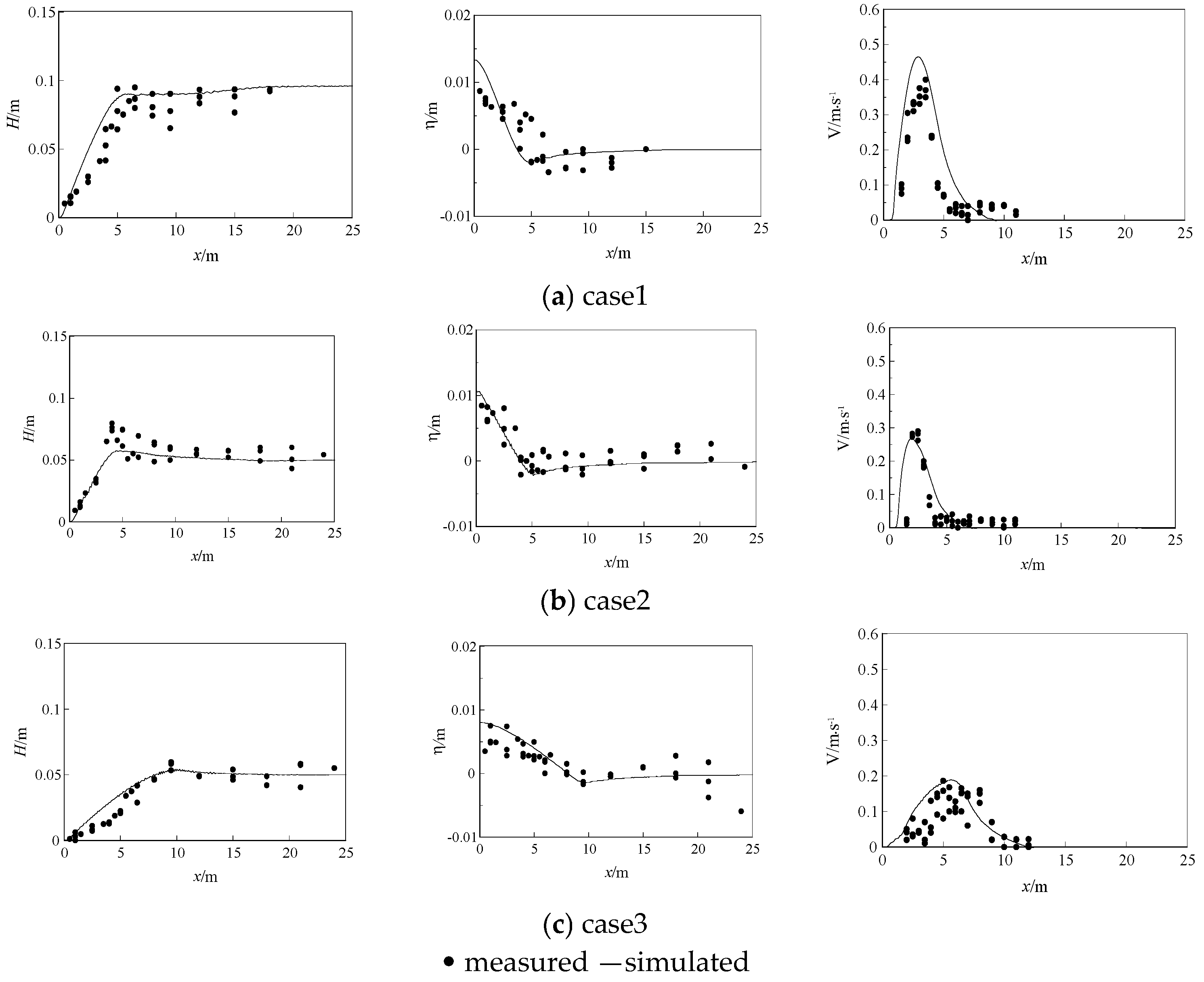
3.1. Validation of Physical Experiments on Nearshore Currents and Pollutant Transport

The State Key Laboratory of Coastal and Offshore Engineering, Dalian University of Technology, in cooperation with Tianjin University, conducted an experimental study on the coastal wave-current fields formed by oblique incident waves and the transport of pollutants in the coastal wave-current fields under the topographic conditions of 1:100 and 1:40 mild slopes. In this paper, the coupled numerical model established above is verified and analyzed with the measured data from this experiment. The plan layout of the experiment is shown in Figure 1. The parameters in the experimental conditions and numerical simulations are shown in

Table 1. Case parameters in the long-shore current and pollutant transport experiment.

Case	Plan Slope	h/m	θ/(°)	H0/m	T/s	γ	Cf	λ	L/m
1	1:40	0.45	0	0.09	1.0	0.65	0.023	0.007	3.0
2	1:40	0.45	0	0.05	2.0	0.65	0.023	0.007	3.0
3	1:100	0.18	0	0.05	2.0	0.60	0.017	0.006	4.5

, where h is the water depth at the wave incidence; θ is the wave incidence angle; H₀ is the incident wave height; T is the incident wave period; γ is the ratio parameter for guiding the breaking waves; C_f is the bottom friction coefficient under wave action; λ is the unfactored amount in the lateral turbulence mixing factor equation; L is the shore distance of the pollutant discharge point.

Figure 2 shows the water depth contour of Case 1. In the numerical calculation, 433 nodes are arranged along the x-direction, and 246 nodes are arranged along the y-direction. The calculation grids layout is shown in Figure 3. The wave is incident along the x-axis in the forward direction. The effective numerical simulation of the nearshore wave-current fields is the basis for the study of nearshore pollutant transport. Figure 4 shows the comparison between the numerical results and the measured data of wave height, water surface elevation, and current velocity [30] for the three conditions in Table 1, respectively. Through numerical comparison between measured and calculated data, the simulation deviation of wave height is approximately 21%, the simulation deviation of water surface elevation is approximately 18%, and the simulation deviation of along-shore flow velocities is approximately 16%. Overall, the numerical solutions generally agree well with the measured data.

Figure 5 shows the distribution of pollutant concentrations at a certain moment, for indicating the location of the pollutant source and the reference position of the pollutant concentration distribution respect to the physical coordinate system. Figure 6, Figure 7 and Figure 8 show the comparison between the numerical results and the measured data of pollutant distribution at several designated moments of three cases in Table 1, where the numerical results are based on the coupled numerical models of nearshore wave-current fields and pollutant transport in the orthogonal curve coordinate system. The left column in Figure 6, Figure 7 and Figure 8 represents the measured values, while the right column represents the simulated values. The curved lines in figures are the pollutant concentration isolines, and the relative minimum value of the pollutant concentration to the discharge point concentration is 10⁻³. From Figure 6, Figure 7 and Figure 8, it can be seen that the pollutant transport trend is basically steady under the certain given wave incidence angle. In Case 1, the incident wave height and current velocity are relatively large, and the pollutant transport velocity is significantly faster than other cases. Compared with Case 2 and Case 3, the pollutant transport velocity is accelerated in the steep slope case under the same wave incidence condition. In general, the numerical results of pollutant distribution at each moment are in good agreement with the distribution trend of the measured data. Due to the difficulty of measurement in the experiment itself and the fact that the numerical results of pollutant distribution are averaged along the vertical direction of water depth, while the measured results are superimposed, these numerical results inevitably have some differences with the measured data.

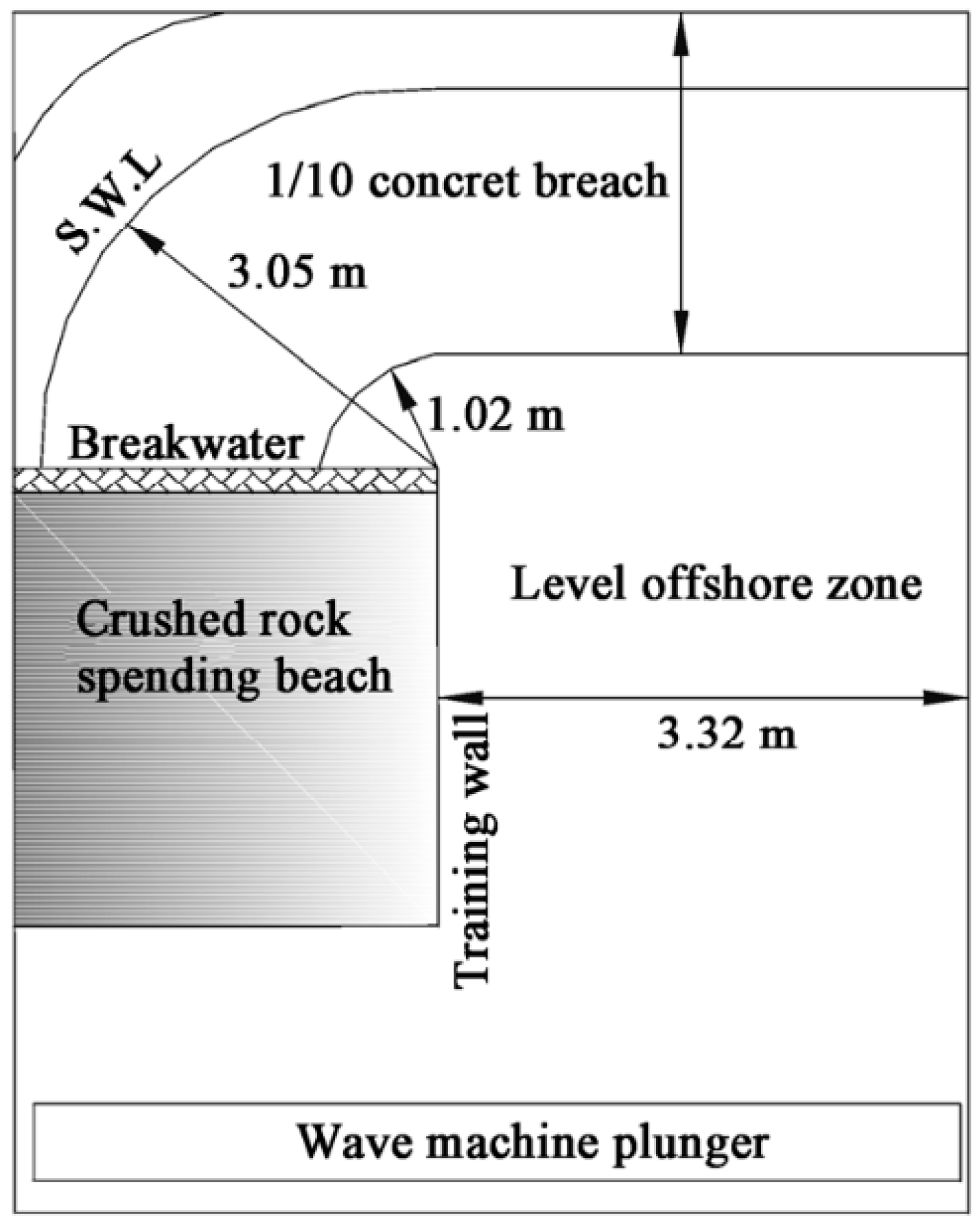
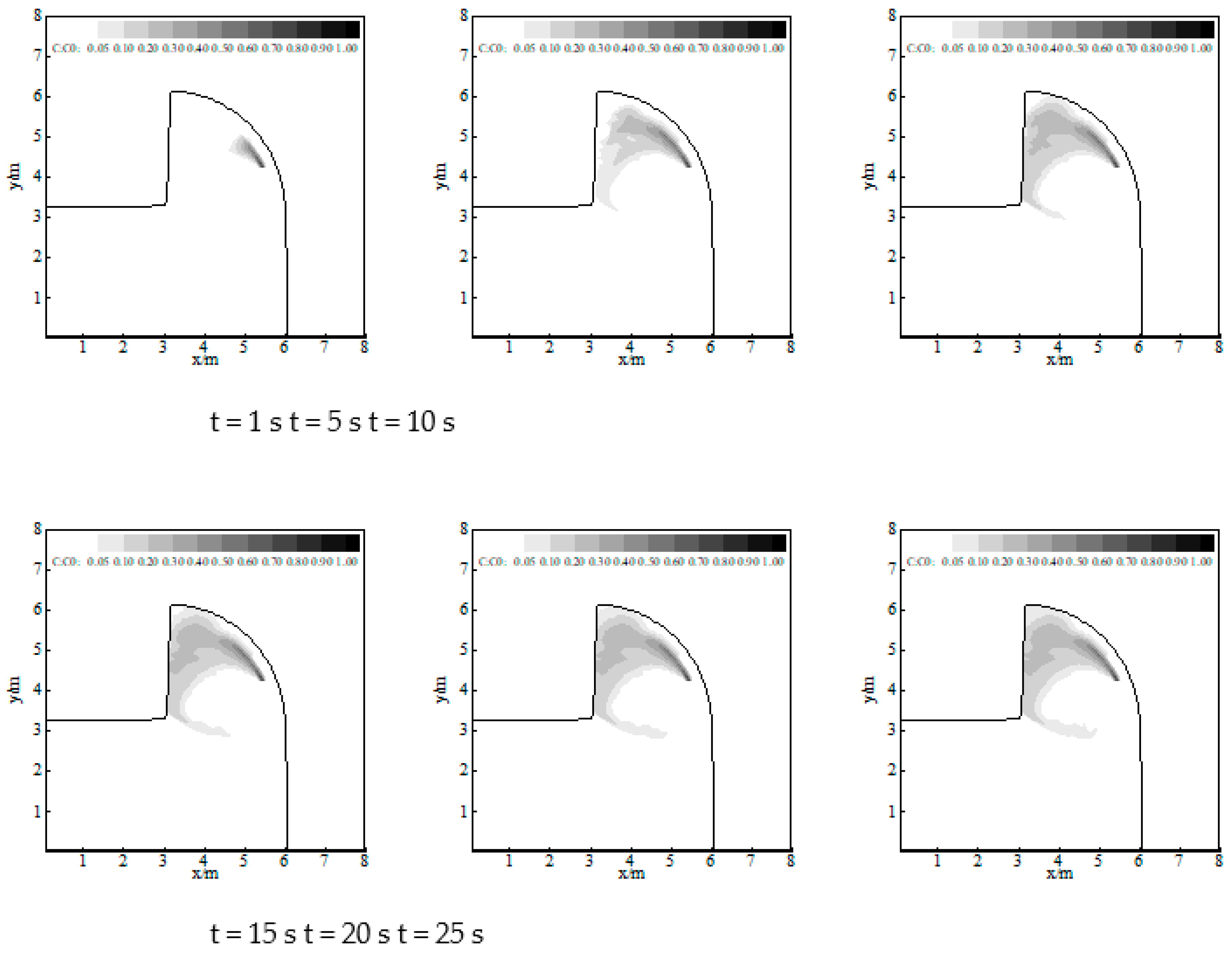
3.2. Numerical Simulation of Pollutant Transport in Gourlay Experiment

The plan layout of the Gourlay [18] experiment is shown in Figure 9. At one end of the wave tank, a pusher-type wavemaker was installed; a rocky wave break was set up in the middle left side of the tank to reduce wave reflection; an upright breakwater was adjacent to the wave break; a slope parallel to the incident wave crest with a gradient of 1/10 was set on the right side of the shallow water area; in the downwind direction of the breakwater, a slope with the same gradient of 1/10 was set at the right corner of the breakwater as the center of the circle, by which the shoreline was parallel to the diffraction wave crest everywhere; the water depth in the flat bottom area was 0.2 m; the intersection angle between the flat tank and the right end of the breakwater was exactly 90°. The grid layout of the computational domain is shown in Figure 10, where the grids are properly smoothed in order to form a better orthogonal grid system and avoid the possible computational errors due to the more abrupt right angle bending [13] at the intersection area of the flat flume and the right end of the breakwater.

To verify the wave propagation in this terrain, the incident wave height was set 9.1 cm and the incident wave period was set 1.54 s for a representative case. Figure 11 shows the wave height distribution of the numerical simulation, from which it can be seen that the incident waves are generated from the lower end of the flat flume, then propagate to the right end of the breakwater and continue to propagate to the mild sloping shallows. In the main propagation direction, the wave height attenuation caused by wave breaking is also obvious. Figure 12 shows the measured wave height distribution for this case and, compared with Figure 11, the numerical results are in good agreement with the measured data.

Gourlay [18] also conducted an experimental study on the nearshore current induced by wave diffraction and breaking through a breakwater. The incident wave height was set 69 mm and the period was set 1.0 s. The grid layout of the computational domain is the same as Figure 9. Figure 13 shows the comparison of mean water level between the numerical results and the measured data. It can be seen from the figure that the water surface is slightly decreasing when the wave arrives at the foot of the slope in the shallow water area through the breakwater, and then the water surface gradually climbs along the slope. Near the middle of the slope, the water surface starts to rise, more than 10 mm relative to the static water surface. In the fan-shaped mild slope downwind area of the breakwater, the water surface has been rising, but the elevation is obviously smaller than that in the shallow water area. In general, the numerical results of water surface elevation and the measured values have a relatively consistent distribution trend. Figure 14 shows the comparison of the numerical results of nearshore current distribution obtained from this paper with the measured data [18] and the numerical results of Nielsen [31]; the three show a good correlation. The nearshore current is mainly distributed as eddies in the mild sloping fan area downwind of the breakwater. The maxima of current velocity obtained from numerical simulations in this paper concentrates at the junction of the fan-shaped mild slope and the flat mild slope, which is consistent with the numerical results of Nielsen [31]. In the wave breaking area, the current motion is relatively complicated due to the intersection of the fan-shaped mild slope and the flat mild slope, and a weak rift flow is formed. The numerical results of this paper are not as obvious as the experimental results on the velocity vector distribution of the vortices in the downwind area under the breakwater, which may be related to the fact that the depth-averaged velocity is obtained from the numerical simulations in this paper, while the measured data are the velocity of a certain place under the water surface. In general, with reference to the measured data [18] and the numerical results of Nielsen [31], the numerical results of this paper are well simulated.

The numerical simulation results of wave-current fields above are used as the dynamic basis to further couple the numerical model of pollutant transport in the curvilinear coordinate system established in this paper, and the pollutant transport of continuous point source has been simulated in this case. Figure 15 shows the numerical results of the pollutant distribution at each moment. The highlighted part in the figure shows the pollutant concentration distribution, and the pollutant edge concentration relative to the discharge point concentration is 10⁻². From the figure, it can be seen that the distribution range of pollutants with relative concentration values above 0.6 is relatively small, mainly concentrated in the area around 1.5 m from the discharge point, while pollutants with relative concentration values between 0.2 and 0.6 occupy a larger distribution range. The pollutants show an obvious rotational development in the fan-shaped mild sloping region depending on the boundary of the computational domain, which is consistent with the eddy motion of the nearshore current in this region. In the process of pollutant transport from the discharge point to the left end of the breakwater, the pollutants show more and more obvious diffusion trend while convective propagation. Especially at the intersection of the fan-shaped mild slope and the left end of the breakwater, the diffusion effect of pollutants distribution is very significant. As can be seen from Figure 14a, this phenomenon is not only related to the diffusion effect in the process of pollutant transport, but also may be related to the presence of small-scale eddy at the intersection leading to the intensification of pollutant diffusion. In the process of pollutants leaving the breakwater and propagating to the upper mild sloping area, the distribution of pollutants becomes significantly narrower, which is not only related to the reduction of pollutants concentration in the area away from the discharge point, but also consistent with the relatively narrow distribution of nearshore currents developing in the same direction in the area. In general, the numerical results of the wav-current fields in this case reasonably explain the pollutant transport phenomenon under this topographic condition.

4. Conclusions

The nearshore waves and current fields included by the wave breaking and other effects are important environmental hydrodynamic factors and play a crucial role in the transport of pollutants. In this paper, a numerical model of nearshore pollutant transport under co-action of waves and currents in the orthogonal curve coordinate system has been obtained by orthogonal curve transformation, and the numerical model of wave propagation based on the parabolic mild slope equation and the numerical model of nearshore current in the orthogonal curve coordinate system have been coupled to establish a systematic numerical model for numerically simulating the transport of pollutant. The numerical results of pollutant distribution have been verified by the experiment of pollutant transport under the co-action of waves and currents conducted at the State Key Laboratory of Coastal and Offshore Engineering of Dalian University of Technology. On this basis, the coupled numerical model has been further applied to simulate and analyze the pollutant transport of Gourlay experiment with complex boundaries, which has shown consistent results with the distribution of nearshore waves and currents. This coupled numerical model of nearshore pollutant transport derived from the parabolic mild slope equation is suitable for large sea area modeling, and has the satisfactory computing efficiency, which determines the expectant prospect in practical projects. The following research on application will be further carried out.

References

1. Qiu, D.H. Science and technology problems in coastal and offshore engineering. J. Dalian Univ. Technol. 2000, 40, 631–637. [Google Scholar]
2. Shen, L.D.; Gui, Q.Q.; Zou, Z.L.; He, L.L.; Chen, W.; Jiang, M.T. Experimental study and numerical simulation of mean longshore current for mild slope. Wave Motion. 2020, 99, 102651. [Google Scholar]
3. Shen, Y.M.; Tang, J.; Zheng, Y.H.; Qiu, D.H. Numerical simulation of wave current field in coastal zone based on parabolic mild slope equation. J. Hydraul. Eng. 2006, 37, 301–307. [Google Scholar]
4. Longuet-Higgins, M.S.; Stewart, R.W. Radiation stress and mass transport in gravity waves, with application to ‘surf beats’. J. Fluid Mech. 1962, 13, 481–504. [Google Scholar] [CrossRef]
5. Tang, J.; Shen, Y.M.; Cui, L.; Zheng, Y.H. Numerical simulation of random wave-induced currents. Chin. J. Theor. Appl. Mech. 2008, 40, 455–463. [Google Scholar]
6. Wen, H.J.; Ren, B.; Dong, P.; Zhu, G.C. Numerical analysis of wave-induced current within the inhomogeneous coral reef using a refined SPH model. Coast. Eng. 2020, 156, 103616. [Google Scholar] [CrossRef]
7. Zheng, Y.H.; Shen, Y.M.; Wu, X.G.; You, Y.G. Determination of wave energy dissipation factor and numerical simulation of wave height in the surf zone. Ocean Eng. 2004, 31, 1083–1092. [Google Scholar] [CrossRef]
8. Zheng, J.H.; Hajime, M. Numerical modeling of multi-directional random wave transformation in wave-current coexisting water areas. Adv. Water Sci. 2008, 19, 78–83. [Google Scholar]
9. Tang, J.; Shen, Y.M.; Qiu, D.H. Numerical study of pollutant movement in waves and wave-induced longshore currents in surf zone. Acta Oceanol. Sin. 2008, 27, 122–131. [Google Scholar]
10. Hsu, C.E.; Hsiao, S.C.; Hsu, J.T. Parametric analyses of wave-Induce nearshore current system. J. Coast. Res. 2017, 33, 795–801. [Google Scholar] [CrossRef]
11. Kirby, J.T. Parabolic wave computations in non-orthogonal coordinate systems. J. Waterw. Port Coast. Ocean Eng. 1988, 114, 673–685. [Google Scholar] [CrossRef]
12. Kirby, J.T.; Dalrymple, R.A.; Kaku, H. Parabolic approximations for water waves in conformal coordinate systems. Coast. Eng. 1994, 23, 185–213. [Google Scholar] [CrossRef]
13. Shi, F.Y.; Dalrymple, R.A.; Kirby, J.T.; Chen, Q.; Kennedy, A. A fully nonlinear Boussinesq model in generalized curvilinear coordinates. Coast. Eng. 2001, 42, 337–358. [Google Scholar] [CrossRef]
14. Gao, J.L.; Ma, X.Z.; Zang, J.; Dong, G.H.; Ma, X.J.; Zhu, Y.Z.; Zhou, L. Numerical investigation of harbor oscillations induced by focused transient wave groups. Coast. Eng. 2020, 158, 103670. [Google Scholar] [CrossRef]
15. Gao, J.L.; Ma, X.Z.; Dong, G.H.; Chen, H.Z.; Liu, Q.; Zang, J. Investigation on the effects of Bragg reflection on harbor oscillations. Coast. Eng. 2021, 170, 103977. [Google Scholar] [CrossRef]
16. Sun, T.; Tao, J.H. Numerical simulation of pollutant transport acted by wave for a shallow water sea bay. Int. J. Numer. Methods Fluids 2006, 51, 469–487. [Google Scholar]
17. Tang, J.; Cui, L. Numerical study of pollutant transport in breaking random waves on mild slope zone. Procedia Environ. Sci. 2010, 2, 274–287. [Google Scholar] [CrossRef]
18. Gourlay, M.R. Wave Generated Currents; University of Queensland: Queensland, Australia, 1978. [Google Scholar]
19. Kirby, J.T. Higher-order approximations in the parabolic equation method for water waves. J. Geophys. Res. 1986, 91, 933–952. [Google Scholar] [CrossRef]
20. Dally, W.R.; Dean, R.G.; Dalrymple, R.A. Wave height verification across beaches of arbitrary profile. J. Geophys. Res. 1985, 90, 11917–11927. [Google Scholar] [CrossRef]
21. Grasmeijer, B.T.; Ruessink, B.G. Modeling of waves and currents in the nearshore parametric vs. probabilistic approach. Coast. Eng. 2003, 49, 185–207. [Google Scholar] [CrossRef]
22. Zhang, H.S.; Ding, P.X.; Zhao, H.J. Numerical simulation model of wave propagation in curvilinear coordinates. Acta Oceanol. Sin. 2003, 25, 110–119. [Google Scholar]
23. Lu, Y.J.; Zuo, L.Q.; Shao, X.J.; Wang, H.C.; Li, H.L. A 2D mathematical model for sediment transport by waves and tidal currents. China Ocean Eng. 2005, 19, 571–586. [Google Scholar]
24. Longuet-Higgins, M.S. Longshore currents generated by obliquely incident sea waves, 1 and 2. J. Geophys. Res. 1970, 75, 6778–6789. [Google Scholar] [CrossRef]
25. Jin, Z.Q. A hybrid turbulence model for numerical solution of longshore current and rip current. J. Hohai Univ. 1988, 16, 76–85. [Google Scholar]
26. Katopodi, I.; Ribberink, J.S. Quasi-3D modeling of suspended sediment transport by currents and waves. Coast. Eng. 1992, 18, 83–110. [Google Scholar] [CrossRef]
27. Van-Rijin, L.C. Sedimentation of dredged channels by currents and waves. J. Waterw. Port Coast. Ocean Eng. 1986, 112, 541–559. [Google Scholar] [CrossRef]
28. Falconer, R.A. Water quality simulation study of a natural harbor. J. Waterw. Port Coast. Ocean Eng. 1986, 112, 15–34. [Google Scholar] [CrossRef]
29. Elder, J.W. Computational Hydraulics; Pitman Publishing Limited: London, UK, 1979. [Google Scholar]
30. Zou, Z.L.; Chang, M.; Qiu, D.H.; Wang, F.L.; Dong, G.H. Experimental study of longshore currents. J. Hydrodyn. Ser. A. 2002, 17, 174–180. [Google Scholar]
31. Nielsen, C.; Apelt, C. The application of wave induced forces to a two-dimensional finite element long wave hydrodynamic model. Ocean Eng. 2003, 30, 1233–1251. [Google Scholar] [CrossRef]
Figure 1. Layout of experiment (unit/m).
Water 15 03251 g001
Figure 2. The calculation field and contour.
Water 15 03251 g002
Figure 3. Orthogonal calculation grids.
Water 15 03251 g003
Figure 4. Comparison of simulated and measured wave height, surface elevation, and current ve−locity (a) Case1, (b) Case2, (c) Case3.
Water 15 03251 g004
Figure 5. The distribution of pollutant concentrations at a certain moment.
Water 15 03251 g005
Figure 6. Comparison of the simulated and measured data of the pollutant concentration field in Case 1.
Water 15 03251 g006
Figure 7. Comparison of the simulated and measured data of the pollutant concentration field in Case 2.
Water 15 03251 g007
Figure 8. Comparison of the simulated and measured data of the pollutant concentration field in Case 3.
Water 15 03251 g008
Figure 9. Layout of Gourlay experiment [16].
Water 15 03251 g009
Figure 10. Orthogonal calculation grids. (The grid density used in the numerical calculations is three times the grid shown in this figure).
Water 15 03251 g010
Figure 11. Contour plot of calculated wave height (unit/cm).
Water 15 03251 g011
Figure 12. Observed wave height in Gourlay experiment (unit/cm).
Water 15 03251 g012
Figure 13. Comparison of mean water level.
Water 15 03251 g013
Figure 14. Comparison of velocity vectors (a) Gourlay experimental results, (b) Nielsen [31] numerical results, (c) Numerical results in this paper.
Water 15 03251 g014
Figure 15. The simulated results of pollutant concentration.
Water 15 03251 g015