

Simulation and Reconstruction of Runoff in the High-Cold Mountains Area Based on Multiple Machine Learning Models
 , , ,
, , ,
Abstract
:1. Introduction
2. Research Area and Data
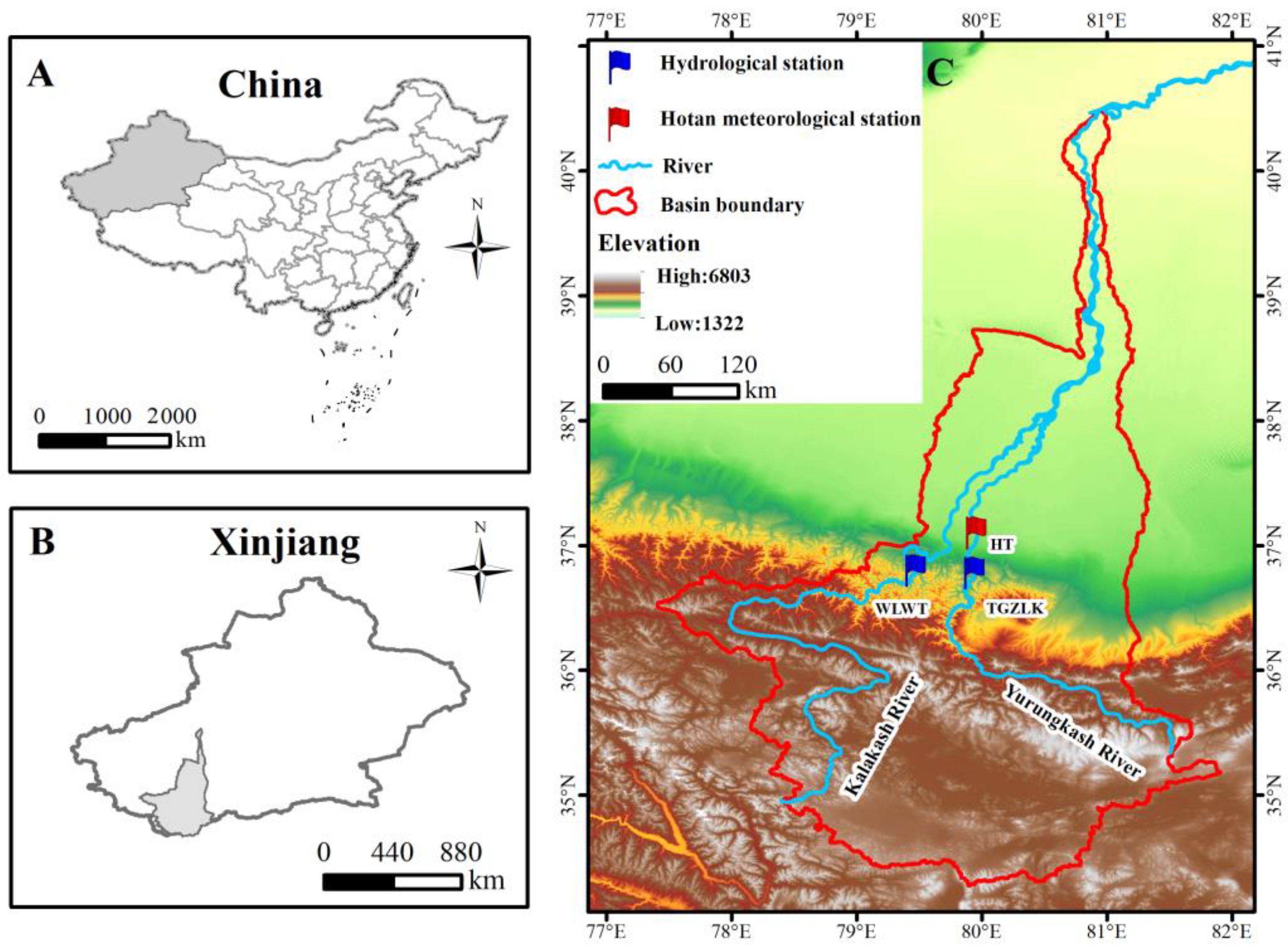
2.1. Research Area
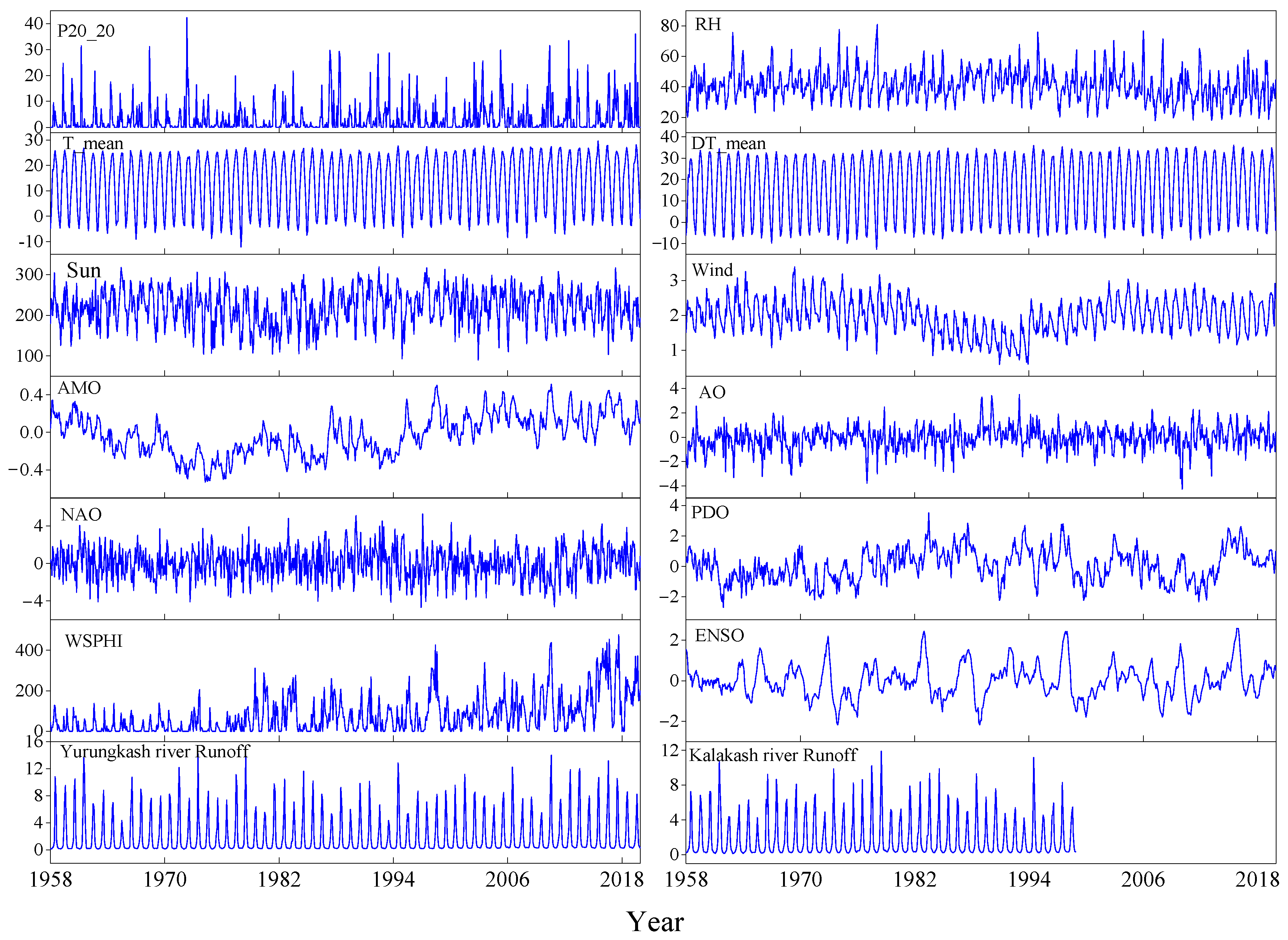
2.2. Data
3. Research Methods
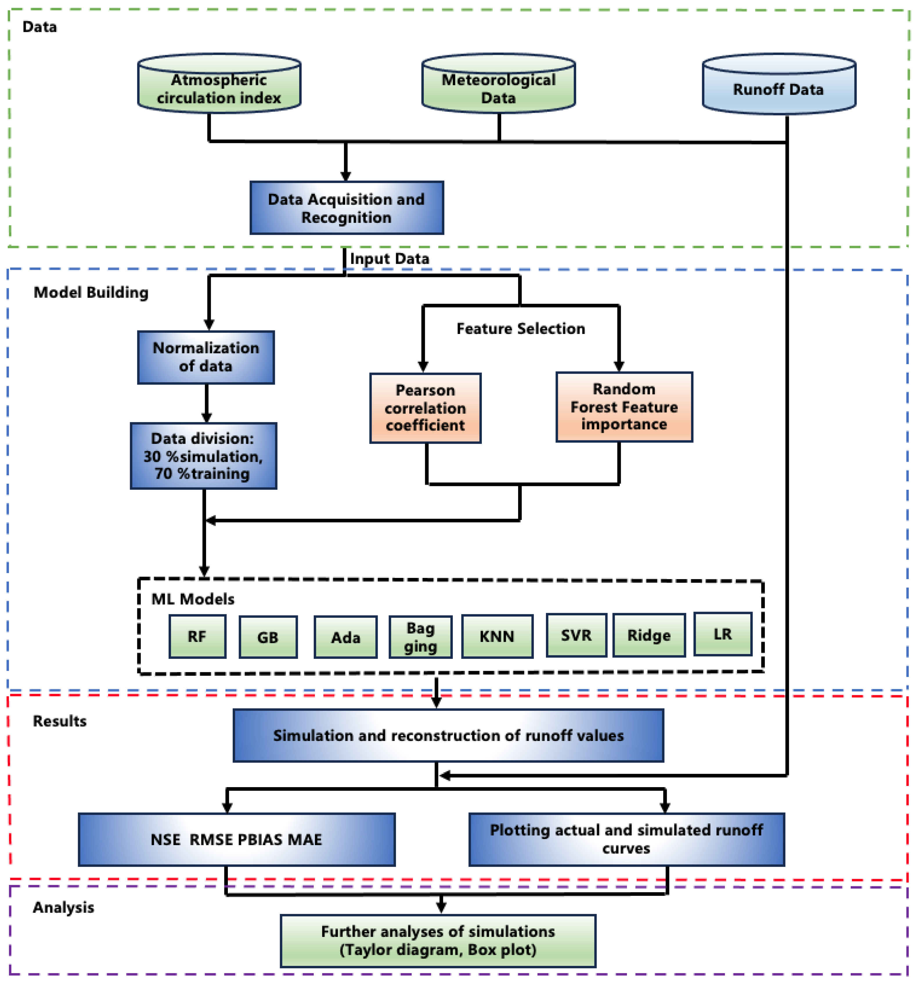
3.1. Runoff Simulation and Reconstruction Modelling
3.2. Feature Selection
3.3. Evaluation Parameters
4. Results and Analyses
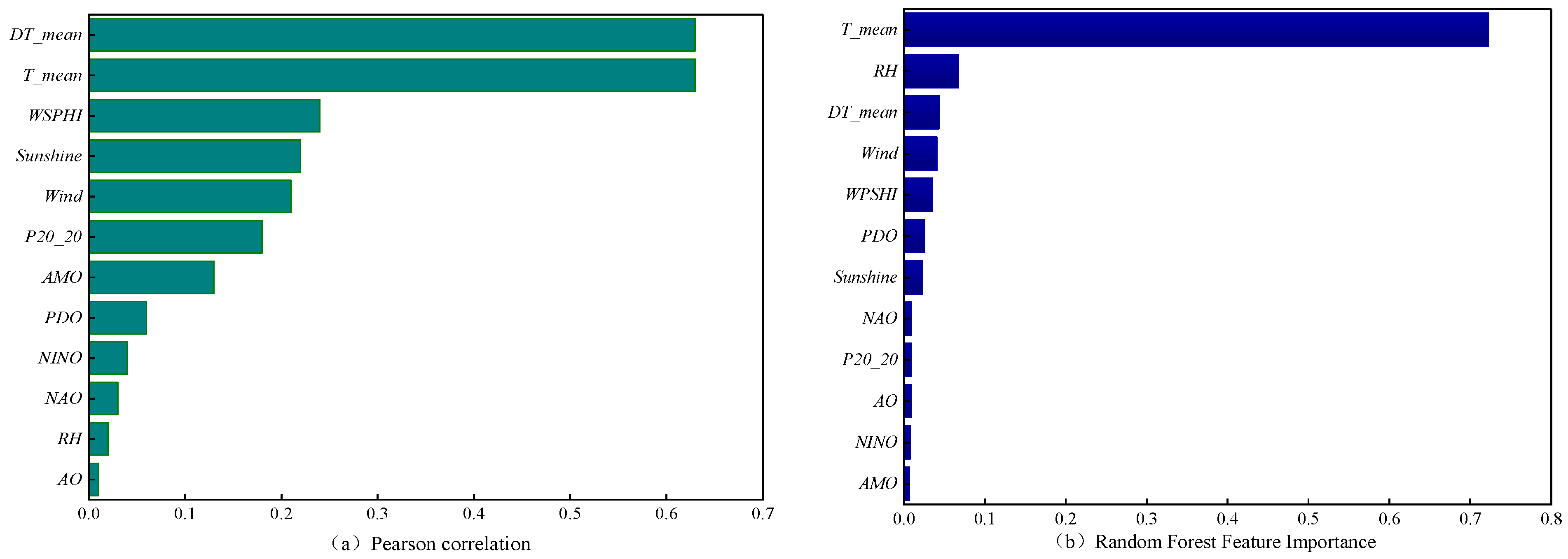
4.1. Feature Analysis
4.1.1. Pearson Correlation Coefficient
4.1.2. Random Forest Feature Importance
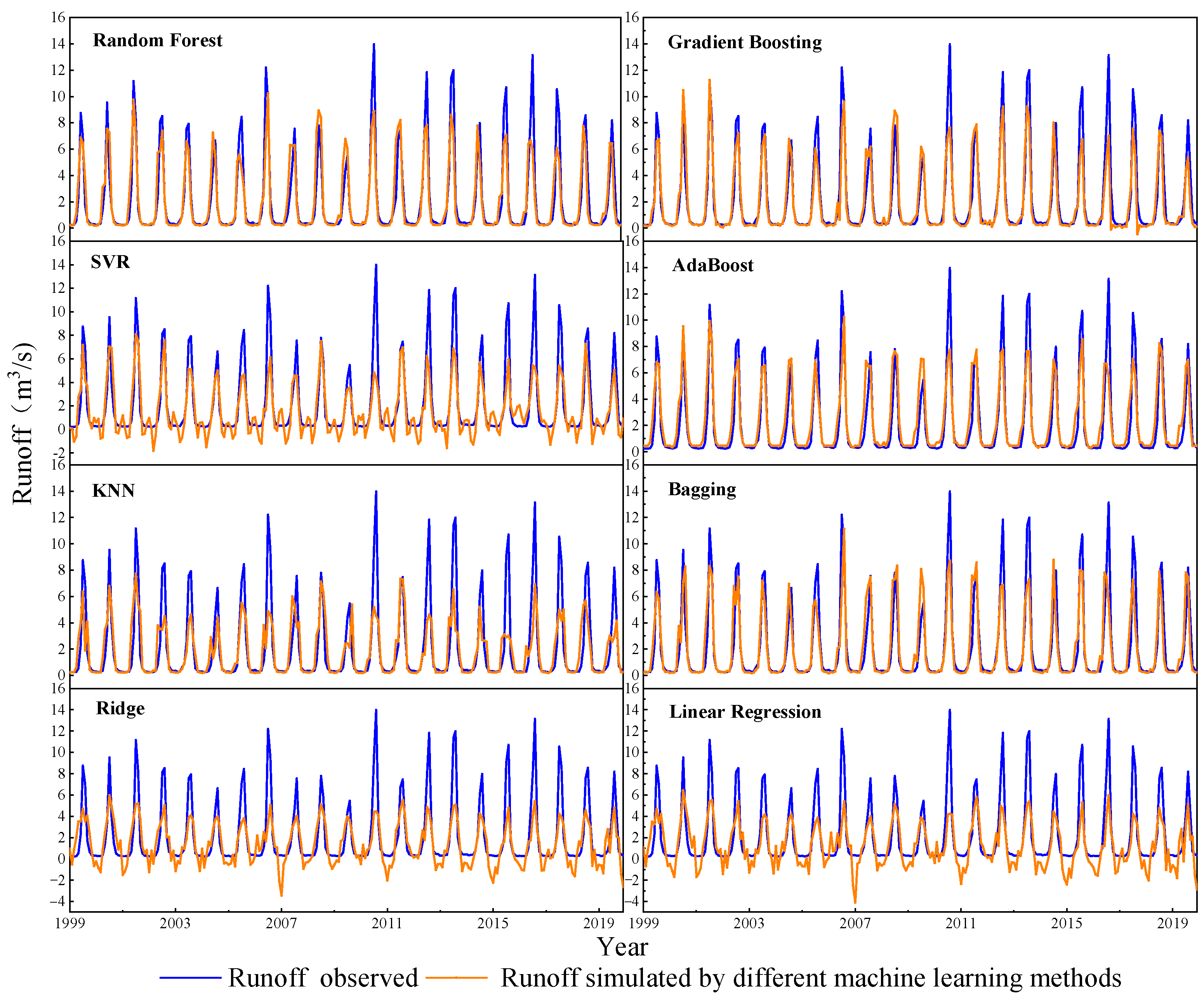
4.2. Runoff Simulation of the Yurungkash River
4.3. Runoff Simulation and Reconstruction of the Kalakash River
4.3.1. Runoff Simulation of the Kalakash River
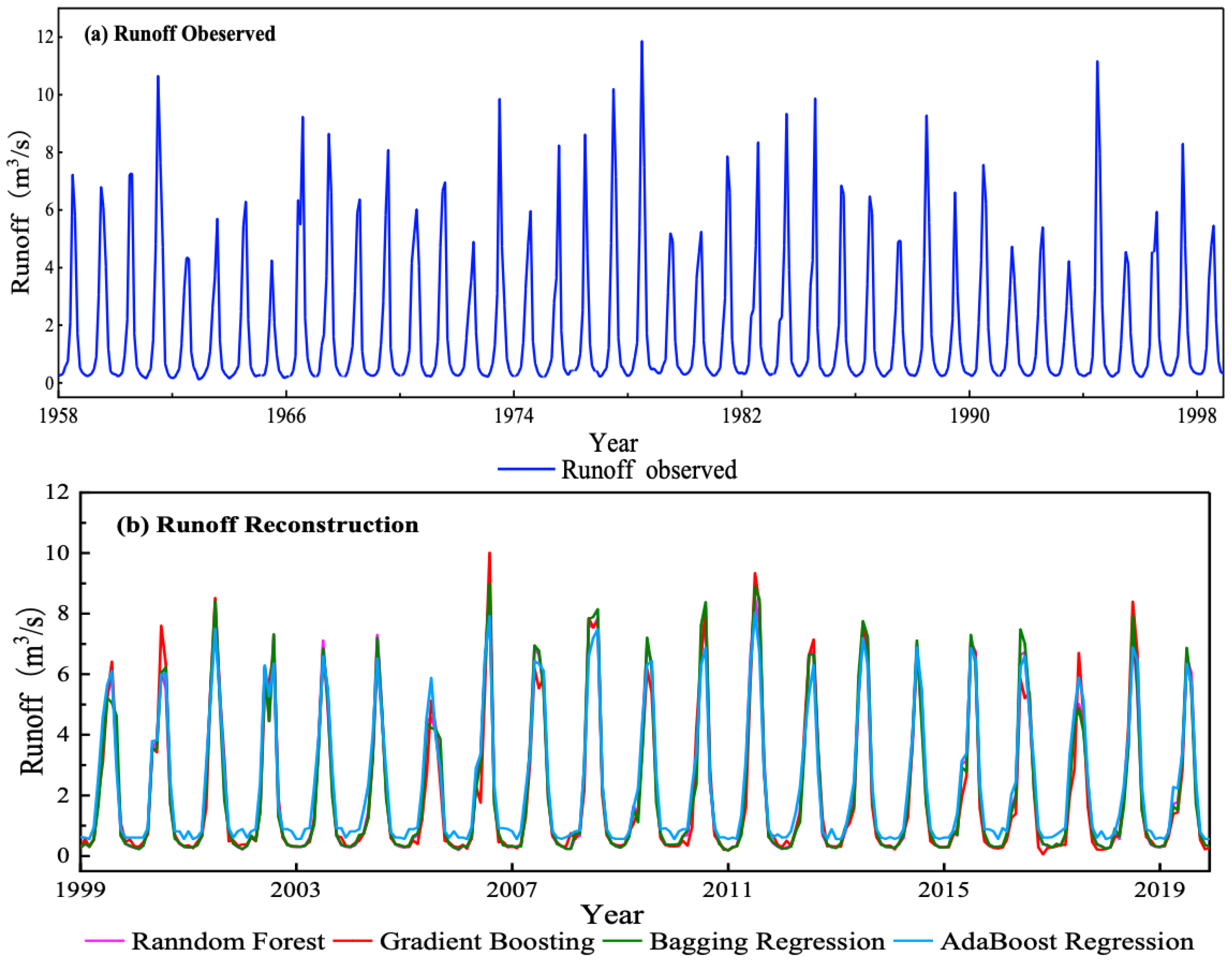
4.3.2. Runoff Reconstruction of the Kalakash River
5. Discussion
6. Conclusions
- (1)
- Temperature is the most important driver of runoff changes in the mountainous areas upstream of the Hotan River, followed by precipitation, hours of sunshine, wind speed, and weak correlation of atmospheric circulation. The random forest features were ranked in order of importance as T_mean > RH > DT_mean > Wind > WSPHI > PDO > Sun > NAO > P20_20 > AO > ENSO > AMO, with a total of 12 elements selected as the machine learning training input data.
- (2)
- Machine learning (ML) methods can successfully simulate runoff changes in the HCMA. Comprehensive runoff curve coincidence and evaluation parameters using gradient boosting, random forest, AdaBoost, and bagging showed obvious advantages over several other ML methods with NSE of 0.84, 0.82, 0.78, and 0.78, respectively, and the other four methods performed the simulation poorly.
- (3)
- The four methods including random forest were applied to simulate the runoff of the Kalakash River from 1978 to 1998 with good results, and the Nash–Sutcliffe efficiency coefficients exceeded 0.75. The reconstruction results of the runoff data of the missing period (1999–2019) reflected the intra-annual and inter-annual variations of the runoff characteristics.
Author Contributions
Funding
Data Availability Statement
Acknowledgments
Conflicts of Interest
Appendix A

| ML Models | Parameters |
|---|---|
| Random Forest | Bootstrap = True, criterion = ‘mse’, max_depth = 100, max_samples = 490, n_estimators = 1000, random_state = 99 |
| Gradient Boosting | n_estimators = 2000, learning_rate = 0.01, max_depth = 15, max_features = ‘sqrt’, alpha = 0.9 |
| SVR | Verbose = False, degree = 3, coef0 = 0.0, kernel = ‘rbf’, tol = 0.001, epsilon = 0.1, max_iter = −1, shrinking = True, cache_size = 200 |
| AdaBoost | n_estimators = 50, learning_rate = 1.0, random_stat e = None, base_estimator = None, loss = ‘linear’ |
| KNN | n_neighbors = 4, weights = ‘uniform’, metric_params = None, n_jobs = None, p = 2, algorithm = ‘auto’ |
| Bagging | n_estimators = 90, oob_score = True, random_state = 90, max_samples = 490 |
| Ridge | Normalize = False, fit_intercept = True, alpha = 1.0, copy_X = True, max_iter = None, tol = 0.001, solver = ‘auto’, random_state = None |
| Linear Regression | fit_intercept = True, normalize = False, copy_X = True, n_jobs = None, positive = False |
References
- Luo, M.; Liu, T.; Meng, F.; Duan, Y.; Bao, A.; Xing, W.; Feng, X.; De Maeyer, P.; Frankl, A. Identifying climate change impacts on water resources in Xinjiang, China. Sci. Total Environ. 2019, 676, 613–626. [Google Scholar] [CrossRef] [PubMed]
- Rangecroft, S.; Harrison, S.; Anderson, K.; Magrath, J.; Castel, A.P.; Pacheco, P. Climate change and water resources in arid mountains: An example from the Bolivian Andes. Ambio 2013, 42, 852–863. [Google Scholar] [CrossRef] [PubMed]
- Zhang, J.; Xu, B.; Gu, Z.; Lv, Y.; Yin, Z.; Guo, X.; Li, L. Coupling of river discharges and alpine glaciers in arid Central Asia. Quat. Int. 2023, 667, 19–28. [Google Scholar] [CrossRef]
- Yang, B.; Du, W.; Li, J.; Bao, A.; Ge, W.; Wang, S.; Lyu, X.; Gao, X.; Cheng, X. The Influence of Glacier Mass Balance on River Runoff in the Typical Alpine Basin. Water 2023, 15, 2762. [Google Scholar] [CrossRef]
- Wang, C.; Xu, J.; Chen, Y.; Bai, L.; Chen, Z. A hybrid model to assess the impact of climate variability on streamflow for an ungauged mountainous basin. Clim. Dyn. 2018, 50, 2829–2844. [Google Scholar] [CrossRef]
- Jiang, J.; Cai, M.; Xu, Y.; Fang, G. The changing trend of flooding in the Aksu River basin. J. Glaciol. Geocryol 2021, 43, 1–10. [Google Scholar]
- Wang, X.; Chen, R.; Li, K.; Yang, Y.; Liu, J.; Liu, Z.; Han, C. Trends and Variability in Flood Magnitude: A Case Study of the Floods in the Qilian Mountains, Northwest China. Atmosphere 2023, 14, 557. [Google Scholar] [CrossRef]
- Sommer, C.; Malz, P.; Seehaus, T.C.; Lippl, S.; Zemp, M.; Braun, M.H. Rapid glacier retreat and downwasting throughout the European Alps in the early 21st century. Nat. Commun. 2020, 11, 3209. [Google Scholar] [CrossRef]
- Wang, J.; Liu, D.W.; Tian, S.N.; Ma, J.L.; Wang, L.X. Coupling reconstruction of atmospheric hydrological profile and dry-up risk prediction in a typical lake basin in arid area of China. Sci. Rep. 2022, 12, 6535. [Google Scholar] [CrossRef]
- Mo, K.L.; Chen, Q.W.; Chen, C.; Zhang, J.Y.; Wang, L.; Bao, Z.X. Spatiotemporal variation of correlation between vegetation cover and precipitation in an arid mountain-oasis river basin in northwest China. J. Hydrol. 2019, 574, 138–147. [Google Scholar] [CrossRef]
- Yan, L.; Lei, Q.W.; Jiang, C.; Yan, P.T.; Ren, Z.; Liu, B.; Liu, Z.J. Climate-informed monthly runoff prediction model using machine learning and feature importance analysis. Front. Environ. Sci. 2022, 10, 1049840. [Google Scholar] [CrossRef]
- Xiao, C.; Zhong, Y.; Wu, Y.; Bai, H.; Li, W.; Wu, D.; Wang, C.; Tian, B. Applying Reconstructed Daily Water Storage and Modified Wetness Index to Flood Monitoring: A Case Study in the Yangtze River Basin. Remote Sens. 2023, 15, 3192. [Google Scholar] [CrossRef]
- Wang, F.; Shao, W.; Yu, H.J.; Kan, G.Y.; He, X.Y.; Zhang, D.W.; Ren, M.L.; Wang, G. Re-evaluation of the power of the mann-kendall test for detecting monotonic trends in hydrometeorological time series. Front. Earth Sci. 2020, 8, 14. [Google Scholar] [CrossRef]
- Abebe, S.A.; Qin, T.; Zhang, X.; Yan, D. Wavelet transform-based trend analysis of streamflow and precipitation in Upper Blue Nile River basin. J. Hydrol. Reg. Stud. 2022, 44, 101251. [Google Scholar] [CrossRef]
- Huang, T.T.; Wang, Z.H.; Wu, Z.Y.; Xiao, P.Q.; Liu, Y. Attribution analysis of runoff evolution in Kuye River Basin based on the time-varying budyko framework. Front. Earth Sci. 2023, 10, 1092409. [Google Scholar] [CrossRef]
- Quang, N.H.; Loc, H.H.; Park, E. Characterizing sediment load variability in the red river system using empirical orthogonal function analysis: Implications for water resources management in data poor regions. J. Hydrol. 2023, 624, 129891. [Google Scholar] [CrossRef]
- Feng, Z.; Niu, W.; Tang, Z.; Xu, Y.; Zhang, H. Evolutionary artificial intelligence model via cooperation search algorithm and extreme learning machine for multiple scales nonstationary hydrological time series prediction. J. Hydrol. 2021, 595, 126062. [Google Scholar] [CrossRef]
- Amiri, S.N.; Khoshravesh, M.; Valashedi, R.N. Assessing the effect of climate and land use changes on the hydrologic regimes in the upstream of Tajan river basin using SWAT model. Appl. Water Sci. 2023, 13, 130. [Google Scholar] [CrossRef]
- Zhao, Y.; Chen, Y.; Zhu, Y.; Xu, S. Evaluating the Feasibility of the Liuxihe Model for Forecasting Inflow Flood to the Fengshuba Reservoir. Water 2023, 15, 1048. [Google Scholar] [CrossRef]
- Liu, J.; Liu, T.; Bao, A.; De Maeyer, P.; Kurban, A.; Chen, X. Response of hydrological processes to input data in high alpine catchment: An assessment of the Yarkant River Basin in China. Water 2016, 8, 181. [Google Scholar] [CrossRef]
- Luo, M.; Meng, F.; Liu, T.; Duan, Y.; Frankl, A.; Kurban, A.; De Maeyer, P. Multi–model ensemble approaches to assessment of effects of local Climate Change on water resources of the Hotan River Basin in Xinjiang, China. Water 2017, 9, 584. [Google Scholar] [CrossRef]
- He, C.; Chen, F.; Long, A.; Qian, Y.; Tang, H. Improving the precision of monthly runoff prediction using the combined non-stationary methods in an oasis irrigation area. Agric. Water Manag. 2023, 279, 108161. [Google Scholar] [CrossRef]
- Perrin, C.; Oudin, L.; Andreassian, V.; Rojas-Serna, C.; Michel, C.; Mathevet, T. Impact of limited streamflow data on the efficiency and the parameters of rainfall—Runoff models. Hydrol. Sci. J. 2007, 52, 131–151. [Google Scholar] [CrossRef]
- Lu, M.; Hou, Q.; Qin, S.; Zhou, L.; Hua, D.; Wang, X.; Cheng, L. A Stacking Ensemble Model of Various Machine Learning Models for Daily Runoff Forecasting. Water 2023, 15, 1265. [Google Scholar] [CrossRef]
- Mohammadi, B. A review on the applications of machine learning for runoff modeling. Sustain. Water Resour. Manag. 2021, 7, 98. [Google Scholar] [CrossRef]
- Hao, R.; Bai, Z. Comparative Study for Daily Streamflow Simulation with Different Machine Learning Methods. Water 2023, 15, 1179. [Google Scholar] [CrossRef]
- Rizeei, H.M.; Pradhan, B.; Saharkhiz, M.A. An integrated fluvial and flash pluvial model using 2D high-resolution sub-grid and particle swarm optimization-based random forest approaches in GIS. Complex Intell. Syst. 2019, 5, 283–302. [Google Scholar] [CrossRef]
- Langhammer, J. Flood Simulations Using a Sensor Network and Support Vector Machine Model. Water 2023, 15, 2004. [Google Scholar] [CrossRef]
- Vaheddoost, B.; Safari, M.J.S.; Yilmaz, M.U. Rainfall-runoff simulation in ungauged tributary streams using drainage area ratio-based multivariate adaptive regression spline and random forest hybrid models. Pure Appl. Geophys. 2023, 180, 365–382. [Google Scholar] [CrossRef]
- Nasiboglu, R.; Nasibov, E. WABL method as a universal defuzzifier in the fuzzy gradient boosting regression model. Expert Syst. Appl. 2023, 212, 118771. [Google Scholar] [CrossRef]
- Noble, W.S. What is a support vector machine? Nat. Biotechnol. 2006, 24, 1565–1567. [Google Scholar] [CrossRef] [PubMed]
- Ratnasingam, S.; Muñoz-Lopez, J. Distance Correlation-Based Feature Selection in Random Forest. Entropy 2023, 25, 1250. [Google Scholar] [CrossRef]
- Natekin, A.; Knoll, A. Gradient boosting machines, a tutorial. Front. Neurorobotics 2013, 7, 21. [Google Scholar] [CrossRef]
- Niu, W.-J.; Feng, Z.-K.; Xu, Y.-S.; Feng, B.-F.; Min, Y.-W. Improving prediction accuracy of hydrologic time series by least-squares support vector machine using decomposition reconstruction and swarm intelligence. J. Hydrol. Eng. 2021, 26, 04021030. [Google Scholar] [CrossRef]
- Fu, X.; Shen, B.; Dong, Z.; Zhang, X. Assessing the impacts of changing climate and human activities on streamflow in the Hotan River, China. J. Water Clim. Chang. 2020, 11, 166–177. [Google Scholar] [CrossRef]
- Wei, X.; Long, A.; Yin, Z.; Jiawen, Y. Simulation of response of glacier runoff to climate change in the Hotan River Basin. Water Resour. Prot. 2022, 38, 137–144. [Google Scholar]
- Xu, Y. A study of comprehensive evaluation of the water resource carrying capacity in the arid area: A case study in the Hetian river basin of Xinjiang. J. Nat. Resour. 1993, 8, 229–237. [Google Scholar]
- Fan, M.; Xu, J.; Chen, Y.; Li, W. Modeling streamflow driven by climate change in data-scarce mountainous basins. Sci. Total Environ. 2021, 790, 148256. [Google Scholar] [CrossRef]
- Wang, X.; Luo, Y.; Sun, L.; Shafeeque, M. Different climate factors contributing for runoff increases in the high glacierized tributaries of Tarim River Basin, China. J. Hydrol. Reg. Stud. 2021, 36, 100845. [Google Scholar] [CrossRef]
- Guo, H.; Ling, H.; Xu, H.; Guo, B. Study of suitable oasis scales based on water resource availability in an arid region of China: A case study of Hotan River Basin. Environ. Earth Sci. 2016, 75, 984. [Google Scholar] [CrossRef]
- Tan, K.; Wang, X.; Gao, H. Analysis of ecological effects of comprehensive treatment in the Tarim River Basin using remote sensing data. Min. Sci. Technol. 2011, 21, 519–524. [Google Scholar] [CrossRef]
- Xue, X.; Mi, Y.; Li, Z.; Chen, Y. Long-term trends and sustainability analysis of air temperature and precipitation in the Hotan River Basin. Resour. Sci. 2008, 30, 1833–1838. [Google Scholar]
- Luo, M.; Liu, T.; Meng, F.; Duan, Y.; Huang, Y.; Frankl, A.; De Maeyer, P. Proportional coefficient method applied to TRMM rainfall data: Case study of hydrological simulations of the Hotan River Basin (China). J. Water Clim. Chang. 2017, 8, 627–640. [Google Scholar] [CrossRef]
- Liu, P.; Jiang, Z.; Li, Y.; Lan, F.; Sun, Y.; Yue, X. Quantitative Study on Improved Budyko-Based Separation of Climate and Ecological Restoration of Runoff and Sediment Yield in Nandong Underground River System. Water 2023, 15, 1263. [Google Scholar] [CrossRef]
- Nuber, S.; Rae, J.W.; Zhang, X.; Andersen, M.B.; Dumont, M.D.; Mithan, H.T.; Sun, Y.; De Boer, B.; Hall, I.R.; Barker, S. Indian Ocean salinity build-up primes deglacial ocean circulation recovery. Nature 2023, 617, 306–311. [Google Scholar] [CrossRef] [PubMed]
- Ye, Y.; Li, Z.; Li, X.; Li, Z. Projection and Analysis of Floods in the Upper Heihe River Basin under Climate Change. Atmosphere 2023, 14, 1083. [Google Scholar] [CrossRef]
- Zhang, Q.; Shen, Z.; Pokhrel, Y.; Farinotti, D.; Singh, V.P.; Xu, C.-Y.; Wu, W.; Wang, G. Oceanic climate changes threaten the sustainability of Asia’s water tower. Nature 2023, 615, 87–93. [Google Scholar] [CrossRef]
- Wang, J.; Sun, X.; Cheng, Q.; Cui, Q. An innovative random forest-based nonlinear ensemble paradigm of improved feature extraction and deep learning for carbon price forecasting. Sci. Total Environ. 2021, 762, 143099. [Google Scholar] [CrossRef] [PubMed]
- Shah, S.H.; Angel, Y.; Houborg, R.; Ali, S.; McCabe, M.F. A random forest machine learning approach for the retrieval of leaf chlorophyll content in wheat. Remote Sens. 2019, 11, 920. [Google Scholar] [CrossRef]
- Nguyen, J.M.; Jézéquel, P.; Gillois, P.; Silva, L.; Ben Azzouz, F.; Lambert-Lacroix, S.; Juin, P.; Campone, M.; Gaultier, A.; Moreau-Gaudry, A. Random forest of perfect trees: Concept, performance, applications and perspectives. Bioinformatics 2021, 37, 2165–2174. [Google Scholar] [CrossRef]
- Saravanan, S.; Abijith, D.; Reddy, N.M.; Parthasarathy, K.; Janardhanam, N.; Sathiyamurthi, S.; Sivakumar, V. Flood susceptibility mapping using machine learning boosting algorithms techniques in Idukki district of Kerala India. Urban Clim. 2023, 49, 101503. [Google Scholar] [CrossRef]
- Friedman, J.H. Greedy function approximation: A gradient boosting machine. Ann. Stat. 2001, 29, 1189–1232. [Google Scholar] [CrossRef]
- Kurani, A.; Doshi, P.; Vakharia, A.; Shah, M. A comprehensive comparative study of artificial neural network (ANN) and support vector machines (SVM) on stock forecasting. Ann. Data Sci. 2023, 10, 183–208. [Google Scholar] [CrossRef]
- Zhong, W.; Du, L. Predicting Traffic Casualties Using Support Vector Machines with Heuristic Algorithms: A Study Based on Collision Data of Urban Roads. Sustainability 2023, 15, 2944. [Google Scholar] [CrossRef]
- Ren, J.; Zhao, H.; Zhang, L.; Zhao, Z.; Xu, Y.; Cheng, Y.; Wang, M.; Chen, J.; Wang, J. Design optimization of cement grouting material based on adaptive boosting algorithm and simplicial homology global optimization. J. Build. Eng. 2022, 49, 104049. [Google Scholar] [CrossRef]
- Wang, C.; Xu, S.; Yang, J. Adaboost algorithm in artificial intelligence for optimizing the IRI prediction accuracy of asphalt concrete pavement. Sensors 2021, 21, 5682. [Google Scholar] [CrossRef] [PubMed]
- Uddin, S.; Haque, I.; Lu, H.; Moni, M.A.; Gide, E. Comparative performance analysis of K-nearest neighbour (KNN) algorithm and its different variants for disease prediction. Sci. Rep. 2022, 12, 6256. [Google Scholar] [CrossRef]
- Wang, F.; Zhen, Z.; Wang, B.; Mi, Z. Comparative study on KNN and SVM based weather classification models for day ahead short term solar PV power forecasting. Appl. Sci. 2017, 8, 28. [Google Scholar] [CrossRef]
- Garcia, S.; Derrac, J.; Cano, J.; Herrera, F. Prototype selection for nearest neighbor classification: Taxonomy and empirical study. IEEE Trans. Pattern Anal. Mach. Intell. 2012, 34, 417–435. [Google Scholar] [CrossRef] [PubMed]
- Rajan, M. An efficient Ridge regression algorithm with parameter estimation for data analysis in machine learning. SN Comput. Sci. 2022, 3, 171. [Google Scholar] [CrossRef]
- Wang, X.; Wang, X.; Ma, B.; Li, Q.; Wang, C.; Shi, Y. High-performance reversible data hiding based on ridge regression prediction algorithm. Signal Process. 2023, 204, 108818. [Google Scholar] [CrossRef]
- Hothorn, T.; Lausen, B. Double-bagging: Combining classifiers by bootstrap aggregation. Pattern Recognit. 2003, 36, 1303–1309. [Google Scholar] [CrossRef]
- Wang, Q.; Luo, Z.; Huang, J.; Feng, Y.; Liu, Z. A novel ensemble method for imbalanced data learning: Bagging of extrapolation-SMOTE SVM. Comput. Intell. Neurosci. 2017, 2017, 1827016. [Google Scholar] [CrossRef] [PubMed]
- James, G.; Witten, D.; Hastie, T.; Tibshirani, R.; Taylor, J. Linear regression. In An Introduction to Statistical Learning:With Applications in Python; Springer: Berlin/Heidelberg, Germany, 2023; pp. 69–134. [Google Scholar]
- Parashar, A.; Parashar, A.; Ding, W.; Shabaz, M.; Rida, I. Data Preprocessing and Feature Selection Techniques in Gait Recognition: A Comparative Study of Machine Learning and Deep Learning Approaches. Pattern Recognit. Lett. 2023, 172, 65–73. [Google Scholar] [CrossRef]
- Wang, W.; Jing, H.; Guo, X.; Dou, B.; Zhang, W. Analysis of Water and Salt Spatio-Temporal Distribution along Irrigation Canals in Ningxia Yellow River Irrigation Area, China. Sustainability 2023, 15, 12114. [Google Scholar] [CrossRef]
- Zhao, Y.; Zhu, W.; Wei, P.; Fang, P.; Zhang, X.; Yan, N.; Liu, W.; Zhao, H.; Wu, Q. Classification of Zambian grasslands using random forest feature importance selection during the optimal phenological period. Ecol. Indic. 2022, 135, 108529. [Google Scholar] [CrossRef]
- Alduailij, M.; Khan, Q.W.; Tahir, M.; Sardaraz, M.; Alduailij, M.; Malik, F. Machine-learning-based DDoS attack detection using mutual information and random forest feature importance method. Symmetry 2022, 14, 1095. [Google Scholar] [CrossRef]
- Fu, H.; Shen, Y.; Liu, J.; He, G.; Chen, J.; Liu, P.; Qian, J.; Li, J. Cloud detection for FY meteorology satellite based on ensemble thresholds and random forests approach. Remote Sens. 2018, 11, 44. [Google Scholar] [CrossRef]
- Han, H.; Morrison, R.R. Improved runoff forecasting performance through error predictions using a deep-learning approach. J. Hydrol. 2022, 608, 127653. [Google Scholar] [CrossRef]
- Vu, M.; Raghavan, S.V.; Liong, S.-Y. SWAT use of gridded observations for simulating runoff–a Vietnam river basin study. Hydrol. Earth Syst. Sci. 2012, 16, 2801–2811. [Google Scholar] [CrossRef]
- Lu, X.; Li, J.; Liu, Y.; Li, Y.; Huo, H. Quantitative Precipitation Estimation in the Tianshan Mountains Based on Machine Learning. Remote Sens. 2023, 15, 3962. [Google Scholar] [CrossRef]
- Yapo, P.O.; Gupta, H.V.; Sorooshian, S. Automatic calibration of conceptual rainfall-runoff models: Sensitivity to calibration data. J. Hydrol. 1996, 181, 23–48. [Google Scholar] [CrossRef]
- Gu, X.; Yang, G.; He, X.; Zhao, L.; Li, X.; Li, P.; Liu, B.; Gao, Y.; Xue, L.; Long, A. Hydrological process simulation in Manas River Basin using CMADS. Open Geosci. 2020, 12, 946–957. [Google Scholar] [CrossRef]
- Lee, J.; Noh, J. Development of a One-Parameter New Exponential (ONE) Model for Simulating Rainfall-Runoff and Comparison with Data-Driven LSTM Model. Water 2023, 15, 1036. [Google Scholar] [CrossRef]
- Xu, Y.; Hu, C.; Wu, Q.; Jian, S.; Li, Z.; Chen, Y.; Zhang, G.; Zhang, Z.; Wang, S. Research on particle swarm optimization in LSTM neural networks for rainfall-runoff simulation. J. Hydrol. 2022, 608, 127553. [Google Scholar] [CrossRef]
- Feng, Z.-K.; Niu, W.-J.; Wan, X.-Y.; Xu, B.; Zhu, F.-L.; Chen, J. Hydrological time series forecasting via signal decomposition and twin support vector machine using cooperation search algorithm for parameter identification. J. Hydrol. 2022, 612, 128213. [Google Scholar] [CrossRef]
- Patro, E.R.; De Michele, C.; Avanzi, F. Future perspectives of run-of-the-river hydropower and the impact of glaciers’ shrinkage: The case of Italian Alps. Appl. Energy 2018, 231, 699–713. [Google Scholar] [CrossRef]
- Taylor, G.P.; Loikith, P.C.; Aragon, C.M.; Lee, H.; Waliser, D.E. CMIP6 model fidelity at simulating large-scale atmospheric circulation patterns and associated temperature and precipitation over the Pacific Northwest. Clim. Dyn. 2023, 60, 2199–2218. [Google Scholar] [CrossRef]
- Fahu, C.; Tingting, X.; Yujie, Y.; Shengqian, C.; Feng, C.; Wei, H.; Jie, C. Discussion on the problem of “warming and humidification” and its future trend in the arid area of Northwest China. Sci. China Earth Sci. 2023, 53, 1246–1262. [Google Scholar] [CrossRef]
- Zhao, Q.; Ye, B.; Ding, Y.; Zhang, S.; Yi, S.; Wang, J.; Shangguan, D.; Zhao, C.; Han, H. Coupling a glacier melt model to the Variable Infiltration Capacity (VIC) model for hydrological modeling in north-western China. Environ. Earth Sci. 2013, 68, 87–101. [Google Scholar] [CrossRef]
- El Bilali, A.; Abdeslam, T.; Ayoub, N.; Lamane, H.; Ezzaouini, M.A.; Elbeltagi, A. An interpretable machine learning approach based on DNN, SVR, Extra Tree, and XGBoost models for predicting daily pan evaporation. J. Environ. Manag. 2023, 327, 116890. [Google Scholar] [CrossRef] [PubMed]
- Li, X.; Zhang, L.; Zeng, S.; Tang, Z.; Liu, L.; Zhang, Q.; Tang, Z.; Hua, X. Predicting Monthly Runoff of the Upper Yangtze River Based on Multiple Machine Learning Models. Sustainability 2022, 14, 11149. [Google Scholar] [CrossRef]
- Wang, G.; Hao, X.; Yao, X.; Wang, J.; Li, H.; Chen, R.; Liu, Z. Simulations of Snowmelt Runoff in a High-Altitude Mountainous Area Based on Big Data and Machine Learning Models: Taking the Xiying River Basin as an Example. Remote Sens. 2023, 15, 1118. [Google Scholar] [CrossRef]
- Tang, H.; Zhang, F.; Zeng, C.; Wang, L.; Zhang, H.; Xiang, Y.; Yu, Z. Simulation of Runoff through Improved Precipitation:The Case of Yamzho Yumco Lake in the Tibetan Plateau. Water 2023, 15, 490. [Google Scholar] [CrossRef]
- Aksan, F.; Suresh, V.; Janik, P.; Sikorski, T. Load Forecasting for the Laser Metal Processing Industry Using VMD and Hybrid Deep Learning Models. Energies 2023, 16, 5381. [Google Scholar] [CrossRef]
- Guo, J.; Liu, Y.; Zou, Q.; Ye, L.; Zhu, S.; Zhang, H. Study on optimization and combination strategy of multiple daily runoff prediction models coupled with physical mechanism and LSTM. J. Hydrol. 2023, 624, 129969. [Google Scholar] [CrossRef]
- Jin, Q.; Sun, Y.; Liu, Z.; He, S. Multidimensional tensor strategy for the inverse analysis of in-service bridge based on SHM data. Innov. Infrastruct. Solut. 2023, 8, 228. [Google Scholar] [CrossRef]
- Khandelwal, A.; Xu, S.; Li, X.; Jia, X.; Stienbach, M.; Duffy, C.; Nieber, J.; Kumar, V. Physics guided machine learning methods for hydrology. arXiv 2020, arXiv:2012.02854. [Google Scholar] [CrossRef]


| River Basin | Lengths (km) | Area (×104 km3) | Temperature (°C) | Precipitation (mm) | Runoff (×108 m3) | Glacier Area (km2) |
|---|---|---|---|---|---|---|
| Yurungkash | 513 | 1.98 | 10.6 | 38.4 | 21.95 | 2958.31 |
| Kalakash | 808 | 2.66 | 11.3 | 36.5 | 21.51 | 2163.17 |
| Data Types | Input Data Name | Time Span | Obtaining Sources |
|---|---|---|---|
| Meteorological data | Air temperature (T_mean) | 1958–2019 | Hotan Meteorological Station (HT) |
| Soil temperature (DT_mean) | |||
| Total precipitation (P20_20) | |||
| Relative humidity (RH) | |||
| Sunshine hours (Sun) | |||
| Wind speed (Wind) | |||
| Hydrological data | Yurungkash River runoff | 1958–2019 | Tongguziluoke Hydrographic Station (TGZLK) |
| Kalakash River runoff | 1958–1998 | Wuluwati Hydrographic Station (WLWT) | |
| Atmospheric circulation data | El Niño-Southern Oscillation (ENSO) | 1958–2019 | Global Climate Observing System (GCOS) https://www.psl.noaa.gov/gcos_wgsp/ (accessed on 5 July 2023) |
| Pacific Decadal Oscillation (PDO) | |||
| Arctic Oscillation (AO) | |||
| Atlantic Multidecadal Oscillation (AMO) | |||
| North Atlantic Oscillation (NAO) | |||
| Western Pacific Subtropical High Pressure Intensity (WPSHI) |
| ML Models | The Core Idea | Strengths and Weaknesses | Reference |
|---|---|---|---|
| Random Forest (RF) | Randomly and independently select a subset of samples to construct multiple decision trees for training, input unknown data, predict each decision tree, and use voting or averaging to obtain the final regression results. | It can better prevent the overfitting phenomenon and overcome the problem of too large a feature dimension, with simple model structure, short training time, high efficiency, strong generalization ability, and good robustness. However, for the sample set with too much data noise, it is easy to produce the overfitting phenomenon. | [48,49,50] |
| Gradient Boosting | The training process first finds a model with weak prediction accuracy, gradually reduces the residuals by adding a predictor, and calculates the residual value between the predicted and actual values of the model to achieve the purpose of improving accuracy, using the iterative principle to use the appropriate loss function, develops a strong learner based on the weak learner, and performs prediction simulation. | The training effect is better, not easy to produce overfitting, with the advantages of high interpretability, high learning efficiency, minimal prediction error, and high stability. However, it requires careful parameter tuning and longer training time. | [51,52] |
| Support Vector Regression (SVR) | Using support vector machines to fit curves for regression analysis, finding a plane to which all the data in the set are closest, minimizing the risk to the expected value, is a machine learning regression algorithm based on support vector machines. | It can effectively solve the regression problem of high-dimensional features, only needing to use part of the support vector to do the decision of the hyperplane, with high accuracy and resolution. However, it is very sensitive to missing data and not very applicable when the sample size is very large. | [53,54] |
| AdaBoost | Multiple weakly learned classifiers are learned by changing the weights of the training samples, and then these weakly learned classifiers are assembled to form a strongest learner for linear fitting to achieve the purpose of predictive simulation. | It can solve multi-class single-label and multi-label problems with high accuracy, highly flexible in use, and fully considers the weight of each classifier. However, the number of classifiers is not well set, and the imbalance of experimental data will lead to a decrease in prediction accuracy and a longer training time. | [55,56] |
| K-Nearest Neighbor (KNN) | KNN scans the set of training samples to find the training sample that is most like the test sample, and then votes to determine the class of the test sample based on the class of the most similar training sample, or votes weighted by the degree of similarity between each sample and the test sample to obtain the result. | KNN is the simplest model in the learner. Based on the KNN regression algorithm, there is no need to consider boundary instances. However, using KNN is more computationally intensive, has low prediction accuracy when the samples are unbalanced, slow to predict, and not very interpretable. | [57,58,59] |
| Ridge | An improvement on the method of least squares estimation. The core idea is to determine the value of the regular term coefficient parameter K. It is dedicated to solving the covariance data partitioning problem and is a regularized regression model. | Enough to effectively reduce the data overfitting phenomenon, the prediction of unknown data is more robust and the obtained regression coefficients are more in line with the mathematical reality, but its fitting ability is easily limited and the underfitting phenomenon may occur. | [60,61] |
| Bagging | The input randomized uniformly selected dataset is trained in multiple rounds to construct weak learners with differences and parallel relationships, which are combined to obtain the final strong learner. | Bagging can be used directly to solve multi-classification and regression problems; by reducing the variance of the classifier, it improves the flourish error and can effectively prevent overfitting. However, underfitting can occur. | [62,63] |
| Linear Regression | Based on regression analysis in mathematics, a straight line is used to describe the relationship more accurately between one or more independent variables and the dependent data. The input data are trained and processed in an algorithmic language to produce a simple prediction value. | The algorithm is simple, fast, and interpretable; however, it can only be used for regression problems, lacks some logic, has a low accuracy of predicted value, and is prone to overfitting. | [64] |
| ML Methods | NSE | PBIAS (%) | RMSE | MAE |
|---|---|---|---|---|
| Random Forest | 0.82 | 4.89 | 1.32 | 0.70 |
| Gradient Boosting | 0.84 | 9.44 | 1.24 | 0.65 |
| SVR | 0.68 | 24.95 | 1.74 | 1.11 |
| AdaBoost | 0.78 | −14.42 | 1.38 | 0.81 |
| KNN | 0.56 | 13.94 | 2.03 | 1.10 |
| Bagging | 0.78 | 11.07 | 1.42 | 0.75 |
| Ridge | 0.53 | 34.13 | 2.11 | 1.42 |
| Linear Regression | 0.51 | 39.99 | 2.14 | 1.48 |
| ML Methods | NSE | PBIAS (%) | RMSE | MAE |
|---|---|---|---|---|
| Random Forest | 0.78 | −19.17 | 1.08 | 0.61 |
| Gradient Boosting | 0.78 | −18.00 | 1.06 | 0.59 |
| Bagging | 0.76 | −19.71 | 1.11 | 0.62 |
| AdaBoost | 0.75 | −31.13 | 1.13 | 0.74 |
Disclaimer/Publisher’s Note: The statements, opinions and data contained in all publications are solely those of the individual author(s) and contributor(s) and not of MDPI and/or the editor(s). MDPI and/or the editor(s) disclaim responsibility for any injury to people or property resulting from any ideas, methods, instructions or products referred to in the content. |
© 2023 by the authors. Licensee MDPI, Basel, Switzerland. This article is an open access article distributed under the terms and conditions of the Creative Commons Attribution (CC BY) license (https://creativecommons.org/licenses/by/4.0/).
Share and Cite
Wang, S.; Sun, M.; Wang, G.; Yao, X.; Wang, M.; Li, J.; Duan, H.; Xie, Z.; Fan, R.; Yang, Y. Simulation and Reconstruction of Runoff in the High-Cold Mountains Area Based on Multiple Machine Learning Models. Water 2023, 15, 3222. https://doi.org/10.3390/w15183222
Wang S, Sun M, Wang G, Yao X, Wang M, Li J, Duan H, Xie Z, Fan R, Yang Y. Simulation and Reconstruction of Runoff in the High-Cold Mountains Area Based on Multiple Machine Learning Models. Water. 2023; 15(18):3222. https://doi.org/10.3390/w15183222
Chicago/Turabian StyleWang, Shuyang, Meiping Sun, Guoyu Wang, Xiaojun Yao, Meng Wang, Jiawei Li, Hongyu Duan, Zhenyu Xie, Ruiyi Fan, and Yang Yang. 2023. "Simulation and Reconstruction of Runoff in the High-Cold Mountains Area Based on Multiple Machine Learning Models" Water 15, no. 18: 3222. https://doi.org/10.3390/w15183222