Runoff Prediction in the Xijiang River Basin Based on Long Short-Term Memory with Variant Models and Its Interpretable Analysis

Abstract

The Long Short-Term Memory (LSTM) neural network model is an effective deep learning approach for predicting streamflow, and the investigation of the interpretability of deep learning models in streamflow prediction is of great significance for model transfer and improvement. In this study, four key hydrological stations in the Xijiang River Basin (XJB) in South China are taken as examples, and the performance of the LSTM model and its variant models in runoff prediction were evaluated under the same foresight period, and the impacts of different foresight periods on the prediction results were investigated based on the SHapley Additive exPlanations (SHAP) method to explore the interpretability of the LSTM model in runoff prediction. The results showed that (1) LSTM was the optimal model among the four models in the XJB; (2) the predicted results of the LSTM model decreased with the increase in foresight period, with the Nash–Sutcliffe efficiency coefficient (NSE) decreasing by 4.7% when the foresight period increased from one month to two months, and decreasing by 3.9% when the foresight period increased from two months to three months; (3) historical runoff had the greatest impact on streamflow prediction, followed by precipitation, evaporation, and the North Pacific Index (NPI); except evaporation, all the others were positively correlated. The results can provide a reference for monthly runoff prediction in the XJB.

1. Introduction

Accurate runoff prediction is the foundation for water resources management, allocation, and utilization, which can provide effective scientific support for regional flood control and drought resistance, the optimization of reservoir scheduling, and the planning and design of hydraulic engineering [1,2,3]. The intricate interplay between climate change and human activities renders runoff formation highly sensitive and results in complex, non-linear, and non-stationary runoff sequences that pose a significant challenge for accurate prediction [4]. Therefore, as runoff patterns become increasingly diverse, it remains a critical focus and challenge in hydrological prediction to explore and develop high-precision runoff prediction models and innovative methods [5,6].

Currently, models used for runoff prediction can be broadly categorized into two types: process-driven models and data-driven models [7,8,9,10,11]. A process-driven model utilizes hydrological cycle analysis and simulation to achieve accurate runoff predictions. While this model can effectively reveal the physical mechanisms of runoff formation, it requires extensive and precise hydrological data. Furthermore, challenges related to model parameter determination and poor generalizability are common [12]. A data-driven model predicts runoff by mining the historical data for relationships between driving factors and target values, offering flexibility in application, remedying the strict requirements of conceptual and physical hydrological models on watershed hydrological conditions, and producing satisfactory simulation results [13,14,15]. As deep learning models continue to advance and computing power improves, the simulation and forecasting capabilities of traditional machine learning have been significantly enhanced. With these advancements, it has become possible to better capture the temporal and spatial structural features in hydrological, meteorological, and geographical data [16,17,18,19,20]. Based on a multi-gate structure, the Long Short-Term Memory (LSTM) network has overcome the problem of vanishing gradients that are commonly encountered in traditional recurrent neural networks and is widely used in the field of runoff prediction [21,22,23,24]. Numerous studies have shown that the LSTM model is not only capable of describing the complex precipitation–runoff relationship of watersheds on a daily scale but also has significant advantages in mining long-term correlations in time series data, particularly in its excellent performance in flood forecasting [25,26,27,28,29]. Besides its ability to mine long-term correlations, the LSTM model boasts structural flexibility. By incorporating other model structures into its standard architecture, such as the Convolutional Neural Network LSTM (CNN-LSTM), Bi-directional LSTM (Bi-LSTM), and Convolutional Long Short-Term Memory (Conv-LSTM), we can create hybrid models that achieve even greater accuracy in prediction [30,31,32,33]. The CNN-LSTM model can combine the characteristics of convolutional neural networks and recurrent neural networks. Barzegar et al. used a CNN-LSTM model to predict water levels in a lake and achieved good results. Their model was able to accurately predict water levels up to two weeks in advance, which could be useful for managing water resources and preventing flooding [34]. Jaseena et al. achieved more reliable and accurate results in wind speed prediction by using the Bi-LSTM model, which uses a bi-directional transmission structure and can comprehensively consider the forward and backward connections of the data [35]. In order to address the problem of spatiotemporal forecasting, a Conv-LSTM hybrid model has been developed with the advantages of spatial feature extraction and learning temporal dependencies in sequential data. Ha et al. developed a Conv-LSTM model to predict the monthly streamflow of the Yangtze River in three flood years [36]. While variant models generated by improving the LSTM model have shown progress in predicting hydrological phenomena, there is currently a lack of a comprehensive evaluation of their performance for streamflow predictions in watersheds. The quantification of the impact of relevant input variables in deep learning-based streamflow simulation, as well as the interpretation of improved streamflow forecasting performance, are still open questions that require further investigation. Although deep learning models have shown good performance in hydrological prediction, their highly non-linear structure makes it difficult to interpret their predictions, which presents some obstacles to the application of these models. Currently, most research efforts in the field of machine learning are focused on improving the predictive performance of deep learning models. However, understanding the rationale behind their predictions remains a major challenge [37,38]. Most of the runoff prediction models built based on machine learning are opaque, with black box or gray box characteristics, and the internal mechanism of the models is unclear. The interpretation is poor, the influence direction of the feature on the output is not clear, and the visibility of the importance of the feature is poor [39,40,41,42]. Common Feature Importance interpretation methods include Feature Importance, Feature Effects, and Feature Interactions. And these have certain applications in hydrology research [43,44]. However, while these methods play an important role in interpretability, they all have different shortcomings. The recent emergence of SHapley Additive exPlanations (SHAP) appears to have changed this situation. SHAP originated from game theory and introduced an additive explanation model, where all features are considered contributors. The response of machine learning output to input can be obtained through calculated SHAP values [45,46]. In addition, the SHAP method has global and local interpretation capabilities, which can provide an explanation of the influence of global features, as well as a local explanation for a single sample or prediction. And the SHAP method has a wide range of applicability, suitable for a variety of machine learning models, including neural networks, decision trees, etc. These advantages can make up for the shortcomings of Feature Importance, Feature Effects, and Feature Interactions. In feature analysis research, SHAP has been proven to be effective in various fields such as medicine [47], automotive engineering [48], materials science [49], and water environment [50,51]. However, to our knowledge, only a few studies have applied interpretable machine learning methods to the attribution analysis of hydrological variables. Moreover, relevant studies have shown that atmospheric circulation is a dominant factor driving climate and weather changes, as well as a key driver of the water cycle, which has a certain impact on streamflow [52,53]. Using an atmospheric circulation factor as the input to the machine learning model not only takes into account the physical factors of runoff formation but also improves the prediction effect of the model [54,55].

The main objectives of this study are the following: (1) to identify the atmospheric circulation factors that have the greatest impact on streamflow and analyze the time-lag effect between historical streamflow, precipitation, evaporation, atmospheric circulation factors, and streamflow forecasts; (2) to investigate the effects of atmospheric circulation factors on streamflow changes in the Xijiang River Basin (XJB) from 1961 to 2018 using the cross-wavelet analysis method; (3) to evaluate the performance of LSTM and its variants in medium- to long-term streamflow prediction by analyzing the impact of different model structures on prediction results under different lead times; (4) to enhance the credibility of the optimal model by conducting interpretability analysis based on SHAP values.

2. Study Area and Data Processing

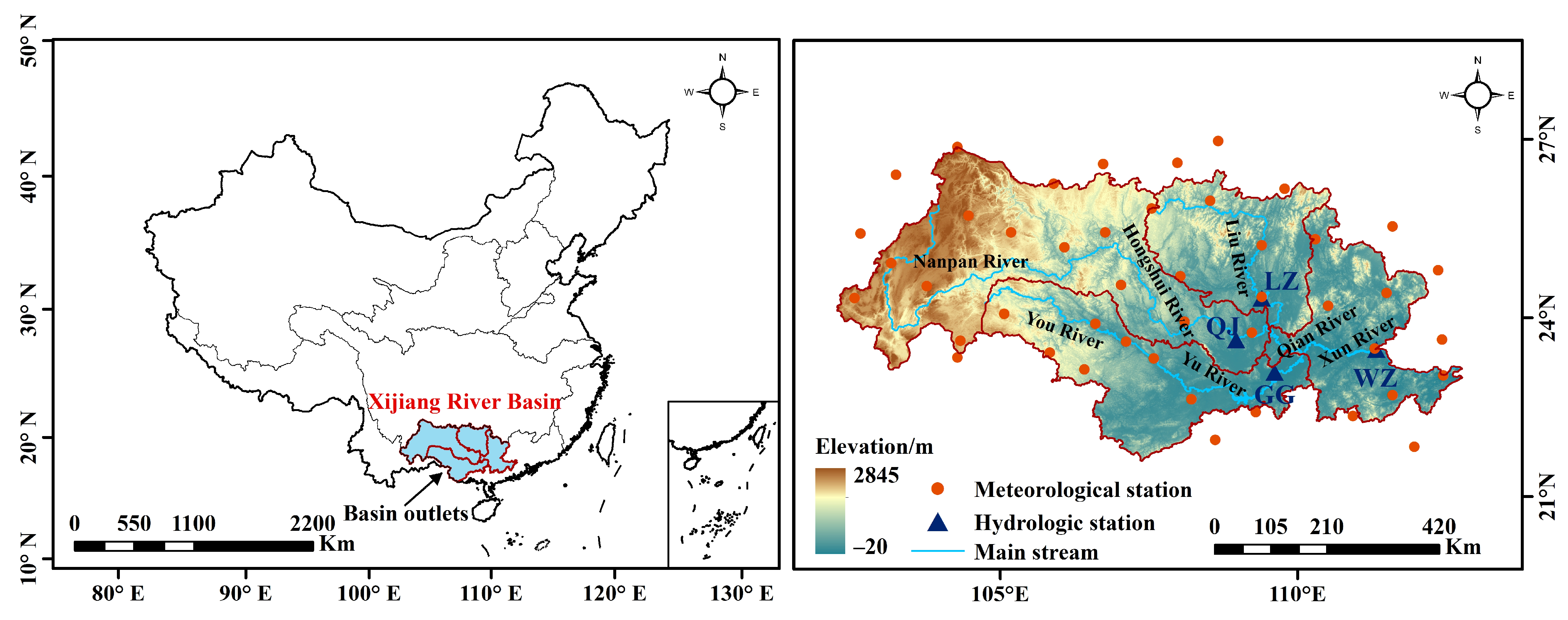
2.1. Study Area

The Xijiang River is the largest tributary of the Pearl River, which originates from Maxiong Mountain, Qujing City, Yunnan Province. It flows into the Pearl River Delta at Sixianjiao, Sanshui, Guangdong Province, with a total length of 2241 km. The main streams from upstream to downstream are the Nanpan River, Hongshui River, Qian River, Xun River, and Xijiang River. The Xijiang River is its general name. The drainage area reaches 353,100 km², 79% of the total area of the Pearl River Basin. The elevation of the basin is high in the Northwest and low in the Southeast. The Yunnan-Guizhou Plateau is in the Northwest, hills and basins are in the middle, and a plain delta is in the East. The terrain of the XJB is complex, and there are significant spatial differences in meteorological and hydrological elements. Based on this, the XJB is divided into four sub-basins: the Upper Xijiang River Basin, the Liu River Basin, the Yu River Basin, and the Middle-Lower Xi River Basin. The hydrological control stations for these sub-basins are Qianjiang (QJ), Liuzhou (LZ), Guigang (GG), and Wuzhou (WZ), respectively.

2.2. Data Processing

The data used in the study consists of observed runoff and meteorological data from various stations, as depicted in Figure 1, spanning the years from 1961 to 2018. Among these, there are missing data for certain months from the LZ station for the period between 1988 and 2000. To address this, missing data for the affected station were interpolated based on concurrent data from downstream stations. Considering the difference of precipitation on the windward slope and the leeward slope in spatial interpolation, Yan et al. [56] showed that the co-Kriging interpolation method of the spherical model and the semi-variance function was adopted in the spatial interpolation of precipitation in Guizhou Province, and better results were obtained. This method considered the influence of the terrain and slope face on precipitation [57]. In addition, the Xijiang River Basin and Guizhou Province have great geographical similarities. Therefore, the collaborative Kriging interpolation method was adopted for spatial interpolation through the software ArcGIS10.3. Furthermore, a rigorous quality control procedure was implemented to ensure data reliability. Regarding atmospheric circulation factors, a set of nine commonly used circulation indices for the same period were chosen as potential factors. These indices include Niño-Southern Oscillation (ENSO), Pacific Decadal Oscillation (PDO), North Atlantic Oscillation (NAO), Arctic Oscillation (AO), Atlantic Multi-decadal Oscillation (AMO), Indian Ocean Dipole Mode Index (DMI), North Pacific Index (NPI), Pacific North American pattern (PNA), and Sunspot Index (SSI) (https://www.ncdc.noaa.gov/teleconnections (accessed on 12 March 2023)).

3. Methodology

3.1. Model Introduction

The LSTM model, as a special type of recurrent neural network, is composed of multiple memory cell structures, each of which is controlled by three “gates” [21]. Figure 2a shows the structure of an LSTM model’s memory cell, where the forget gate f_t determines the amount of previous cell state information to be discarded; the input gate determines the proportion of newly acquired information to be stored in the current cell state C_t; and the output gate O_t determines the final output information at this moment. The specific formulas are as follows:

$$f_t=\sigma (W_f[h_{t-1},x_t]+b_f)$$

(1)

$$i_t=\sigma (W_i[h_{t-1},x_t]+b_i)$$

(2)

$$C_t^{\prime }=tanh(W_c[h_{t-1},x_t]+b_c)$$

(3)

$$C_t=f_t\otimes C_{t-1}+i_t\otimes C_{t-1}^{\prime }$$

(4)

$$O_t=\sigma (W_o[h_{t-1},x_t]+b_o)$$

(5)

$$h_t=o_{t}tanh\otimes C_{t}t$$

(6)

where x_t is the input vector, h_t−1 is the output information of the previous unit state, σ is the sigmoid activation function, $\otimes$ represents the vector multiplication, W_f, W_i, W_c, and W_o are the weight matrices of the neural network, and b_f, b_i, b_c, and b_o are the bias vectors.

In the process of modeling through the software Anaconda2020, by using the method of controlling variables, five hyperparameters of the LSTM model are calibrated, namely time step, dropout rate, batch size, number of units in the hidden layer, and epochs. For each hyperparameter, an initial search space was defined first, and the method of grid search was used to search each hyperparameter, keeping the other hyperparameters unchanged. Through the performance evaluation on the test set, the optimal value of each hyperparameter was selected, other hyperparameters were kept unchanged, the next hyperparameter was added to the adjustment, and the interaction between different hyperparamete was considered. The above steps were repeated until all hyperparameters were calibrated. The final calibration parameters were as follows: time step of 1, batch size of 128, dropout rate of 0.01, 32 units in the hidden layer, and 100 epochs.

The CNN-LSTM model structure, as shown in Figure 2b, combines the CNN and LSTM models. The CNN model extracts and integrates data features through two steps of convolutional kernel pooling, while the LSTM model filters and memorizes the integrated data features before outputting predictions through a fully connected layer [58]. Compared to the LSTM model, the CNN-LSTM model has three additional parameters: filters, convolution kernel size, and pooling layer, all set at 128, (3, 3), and 1, respectively, with other parameters being the same as those of the LSTM model.

The Conv-LSTM model structure, as shown in Figure 2c, aims to establish temporal relationships while characterizing local spatial features. Its internal structure is the same as that of the LSTM model, with the main difference being the calculation method of the “gates”, which is through convolutional calculations for Conv-LSTM and matrix calculations for LSTM [59]. The LSTM model uses one-dimensional input data, which is not suitable for spatial sequence data, whereas the Conv-LSTM model uses two-dimensional input data to overcome this limitation. The Conv-LSTM model has the same parameter types as the CNN-LSTM model, with filters and the convolution kernel size set at 128 and (3, 3), respectively, and other parameters being the same as those of the LSTM model.

The Bi-LSTM model structure, as shown in Figure 2d, processes any sequence forward and backward independently using separate hidden layers. The hidden layers integrate past and future information, giving the Bi-LSTM model the ability to capture data information in both directions [35]. In theory, the Bi-LSTM model can better consider the temporal relationships in runoff data than traditional LSTM models. Apart from the number of hidden layer units, the parameter settings for the Bi-LSTM model are the same as those for the LSTM model. Both sets of hidden layer units are set at 32.

3.2. Wavelet Analysis

The atmospheric circulation is an important factor affecting regional climate change. Its variations and anomalies can simultaneously or sequentially affect distant regions spatially, and the resulting correlation is called teleconnection [60]. Based on wavelet transform and cross-spectrum, the Cross-Wavelet Transform (XWT) method can analyze the multi-time scale teleconnection relationship between two sequences in the time-frequency domain and reveal the phase relationship of the two sequences in the high-energy area [61,62]. The specific principle is as follows: assuming that the two-time sequences are X = {x_i|i = 1, 2, …, n} and Y = {y_i|i = 1, 2, …, n}, their continuous wavelet transforms are $W_n^X(s)$ and $W_n^Y(s)$, respectively. Then, the cross-wavelet spectrum can be defined as follows:

$$W_n^{XY}(s)=W_n^X(s)W_n^{Y*}(s)$$

(7)

where ${ W}_n^{Y*}$(S) is the complex conjugate of ${ W}_n^Y$(S); and ${ W}_n^{XY}$(S) is the absolute value of the cross-wavelet power spectrum.

Although cross-wavelet analysis can reveal the co-localization of two sequences in the high-energy region, its analytical capability for low-energy regions is insufficient [63]. Hence, in this study, wavelet coherence analysis (WTC) was used for analyzing the teleconnection relationship between runoff and atmospheric circulation factors through Matlab2021a software. The specific definition is as follows:

$$R_n^2(n)=\frac{{\left|S\left[s^{-1}{W}_n^{XY}(s)\right]\right|}^2}{S\left[s^{-1}{\left|W_n^X(s)\right|}^2\right]\cdot S\left[s^{-1}{\left|W_n^Y(s)\right|}^2\right]}$$

(8)

where ${\left|S\left[s^{-1}{W}_n^{XY}(s)\right]\right|}^2$ is the cross-product of the fluctuating amplitudes of two time series at a certain frequency; and $S\left[s^{-1}{\left|W_n^X(s)\right|}^2\right]\cdot S\left[s^{-1}{\left|W_n^Y(s)\right|}^2\right]$ is the amplitude of the oscillating waves of two time series.

3.3. Evaluation Indicators

To evaluate the performance of different models in predicting monthly runoff, indicators such as root mean square error (RMSE), mean absolute error (MAE), and the Nash–Sutcliffe efficiency coefficient (NSE) were selected to assess the accuracy of the predictions [64]. As shown in

Table 1. Formulas of evaluation indicators.

Evaluation Indicators	Formula	Optimal Value
RMSE	$RMSE=\sqrt{\frac{1}{n}{\displaystyle \sum {}_{i=1}^n{(Q_f-Q_{obs})}^2}}$	0
MAE	$MAE={\displaystyle \sum _{i=1}^n\left|Q_f-Q_{obs}\right|}/n$	0
NSE	$NSE=1-{\displaystyle \sum _{i=1}^n{\left(Q_f-Q_{obs}\right)}^2}/{\displaystyle \sum _{i=1}^n{\left(Q_{obs}-\overline{Q_{obs}}\right)}^2}$	1

, Q_obs represents the observed values, Q_f represents the predicted values, $\overline{Q_{obs}}$ represents the mean of the observed values, and n is the number of observed values.

3.4. Interpretable Machine Learning Method

One of the limitations of using machine learning models is their lack of interpretability. Specifically, SHAP is an interpretable machine learning method based on game theory that quantifies the impact of each feature on model predictions. By calculating the SHAP value for each feature, we can understand how each feature affects the output of the model in a given input case. SHAP visualization tools help us understand the logic behind model predictions, providing an intuitive way to interpret complex machine-learning models [45]. The SHAP value for each input variable represents the weighted average of its marginal contribution. The SHAP method introduces a Shapley Kernel to approximate Shapley Values, making the calculation feasible. A Shapley Kernel is a weighted kernel function used to calculate the impact of each feature on the predicted value, and its formula is as follows:

$${\varphi }_i(x,f)={\displaystyle \sum {}_{S\subseteq N\backslash \left\{i\right\}}}\frac{\left|S\right|!\left(\left|N\right|-\left|S\right|-1\right)!}{\left|N\right|!}\left[f\left(x_{S\cup \left\{i\right\}}\right)-f(x_S)\right]$$

(9)

where x is the input value of the model, f is the ML model; x_S represents the feature subset S of the input value x; f(x_S) represents the predicted value of the feature subset S; i is the feature to calculate the Shapley Value; N is the feature set; f(x_S∪{i}) represents the predicted value of the feature subset S plus feature i; |S| represents the cardinality of the feature subset S; |N| represents the cardinality of the entire feature set N.

The mathematical formula of the SHAP importance measure is as follows:

$$Mean \left(|SHAP value|\right)=\frac{{\displaystyle {\sum }_{i=1}^N\left|{\varphi }_i(x,f)\right|}}{N}$$

(10)

where Mean(|SHAP value|) represents the average of the absolute values of the Shapley values.

4. Results

4.1. Feature Selection

4.1.1. Selection of Atmospheric Circulation Factors

Taking into account the impact of climate change on runoff, atmospheric circulation factors are introduced to screen out the factors that have a significant impact on runoff, which are then integrated into the runoff prediction model to further improve its accuracy. Currently, there are no specific principles to follow for selecting the input features of a machine learning model. Previous studies have mostly used the correlation coefficient method, which has yielded relatively good results [65]. In view of this, the Pearson correlation coefficients between monthly runoff and nine atmospheric circulation factors with different time delays of 0 to 6 months were calculated, and the factor with the highest correlation coefficient was selected as the input factor for the model from the circulation factors that passed the 0.01 significance test, which was the NPI. In general, NPI is the largest when the delay is 1 month, the Pearson correlation coefficient with a 1-month delay is shown in

Table 2. The correlation coefficient between monthly runoff and atmospheric circulation factors with a 1-month delay.

Hydrological Station	ENSO	PDO	NAO	AO	AMO	DMI	NPI	PNA	SSI
QJ	0.026	0.013	−0.029	0.073	−0.032	−0.015	0.512 **	−0.052	0.018
LZ	0.072	0.055	−0.049	0.087 *	0.026	0.024	0.452 **	−0.088 *	0.034
GG	−0.021	−0.063	−0.042	0.064	−0.028	−0.026	0.487 **	−0.056	0.008
WZ	0.040	0.024	−0.001	0.098 **	−0.031	0.006	0.517 **	−0.087 *	0.021

Note: ** means that the correlation coefficient passed a two-tailed test at the 0.01 significance level; * means that the correlation coefficient passed a two-tailed test at the 0.05 significance level.

.

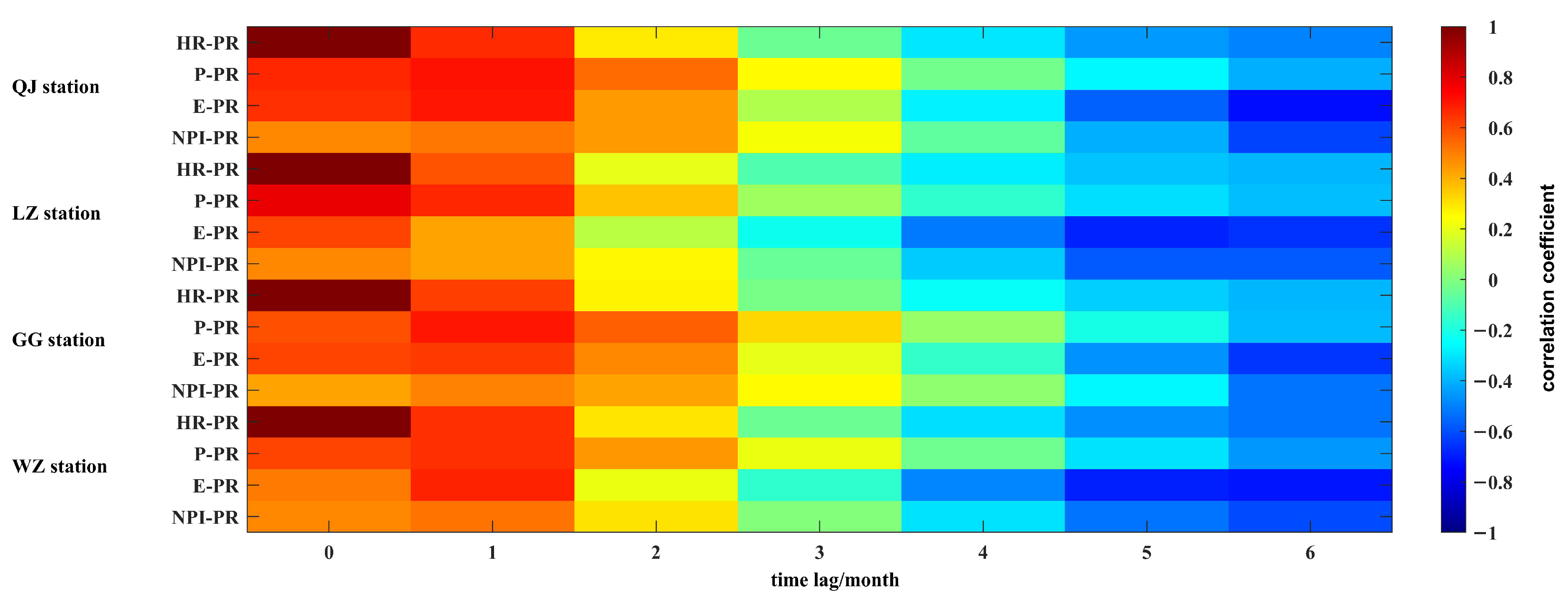
4.1.2. Delayed Effect Analysis

Given the hysteresis effect of factors on runoff, such as precipitation and evaporation, as well as the varying time lags in their impact on runoff, it is critical to analyze and select suitable factors for accurately predicting runoff. The correlation coefficients between precipitation, evaporation, the atmospheric circulation factor NPI, and runoff were calculated at the four hydrological stations of QJ, LZ, GG, and WZ, separately. A correlation coefficient greater than 0.3 can pass a 95% confidence level test, as shown in Figure 3. It was observed that for the QJ station, the 1-month time lag between the historical runoff, precipitation, evaporation, NPI, and predicted runoff showed the highest correlation coefficients, which were 0.66, 0.71, 0.70, and 0.51, respectively. For the LZ station, when the time lag between the historical runoff, precipitation, evaporation, NPI, and predicted runoff was 0 months, the highest correlation coefficients reached 0.58, 0.79, 0.61, and 0.4, respectively. The time lag (1 month) in the GG station was the same as that in the QJ station, with the highest correlation coefficients of 0.62, 0.70, 0.63, and 0.49, respectively. And for the WZ station, the time lag between the historical runoff, precipitation, evaporation, NPI, and predicted runoff was also 1 month, with the highest correlation coefficients of 0.65, 0.66, 0.68, and 0.52, respectively. In addition, when the lag time was 3 months, there was a significant negative correlation between the predicted runoff and various factors. Therefore, based on the comprehensive lag effect analysis, it was determined that all predictive factors should have a consistent time lag of 1 month.

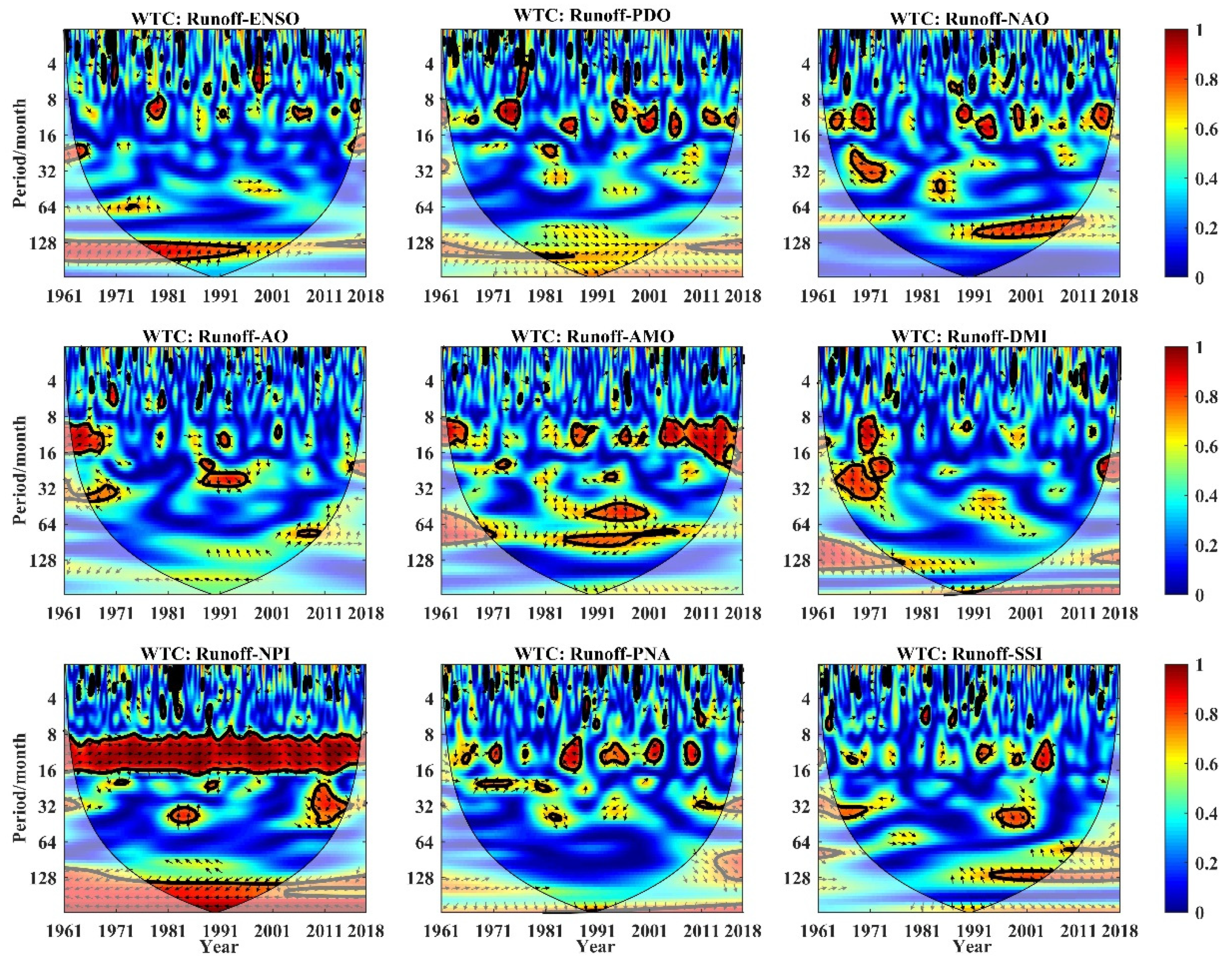
4.2. Driving Effect of Atmospheric Circulation Factors on Runoff Change

In order to explore the main driving factors of monthly runoff variations in the XJB from 1961 to 2018, we adopted a cross-wavelet analysis to further analyze the common characteristics between the monthly runoff and nine atmospheric circulation factors (ENSO, PDO, AO, NAO, AMO, DMI, NPI, PNA, and SSI). Different from the Pearson correlation coefficient method, a cross-wavelet analysis reveals the correlation between two non-stationary signals in both the time domain and frequency domain, which can provide richer feature information than a correlation analysis in the frequency domain. In addition, a cross-wavelet analysis can also reflect the common period between sequences at different scales. The analysis results are shown in Figure 4 and Figure 5 below. Figure 4 shows the cross-wavelet transform diagram of the monthly runoff and atmospheric circulation factors of the WZ station in the low-energy region, that is, in the wavelet condensation spectrum. It can be seen that there is a significant resonance period with a positive correlation between runoff and ENSO, which was 128–190 months in 1973–1995. Runoff and PDO had six significant resonance periods, which were 8–16 months in 1972–1976, 2002–2006, and 2011–2014 with a positive correlation, and 8–16 months in 1983–1987, 1993–1996, and 1998–2002 with a negative correlation, respectively. Runoff and NAO had five significant resonance periods, which were 8–16 months in 1968–1972, and 100–128 months in 1991–2010 with a positive correlation, and 24–40 months in 1967–1972, 1991–1995, and 2011–2010 with a negative correlation, respectively. Runoff and AO had two significant resonance periods with a positive correlation, which were 9–16 months in 1962–1968 and 24–30 months in 1987–1996. Runoff and AMO had three significant resonance periods, which were 48–64 months in 1990–2000 and 8–20 months in 2002–2016 with a positive correlation, and 90–120 months in 1985–1998 with a negative correlation, respectively. Runoff and DMI had two significant resonance periods with a negative correlation, which were 8–16 months in 1968–1972 and 18–40 months in 1964–1975. Runoff and NPI had three significant resonance periods, which were 8–16 months in 1961–2018, 24–48 months in 2009–2015 with a positive correlation, and 128–256 months in 1976–2002 with a negative correlation, respectively. Runoff and PNA had four significant resonance periods with a negative correlation, which were 8–16 months in 1982–1986, 1992–1995, 1998–2003, and 2008–2011. Runoff and SSI had three significant resonance periods, which were 32–48 months in 1995–2001, 10–16 months in 2002–2016 with a positive correlation, and 110–128 months in 1995–2005 with a negative correlation, respectively.

Figure 5 shows the cross-wavelet transform diagram of the monthly runoff and atmospheric circulation factors of the WZ station in the high-energy region, that is, the wavelet energy spectrum. It is worth mentioning that runoff and teleconnection factors (ENSO, PDO, NAO, AO, AMO, DMI, NPI, PNA, SSI) also had short-term intermittent oscillation periods of 8–16 months in 1961–2018, with the NPI having the greatest impact on runoff and showing a positive correlation.

4.3. Comparative Analysis of Model Prediction Performance

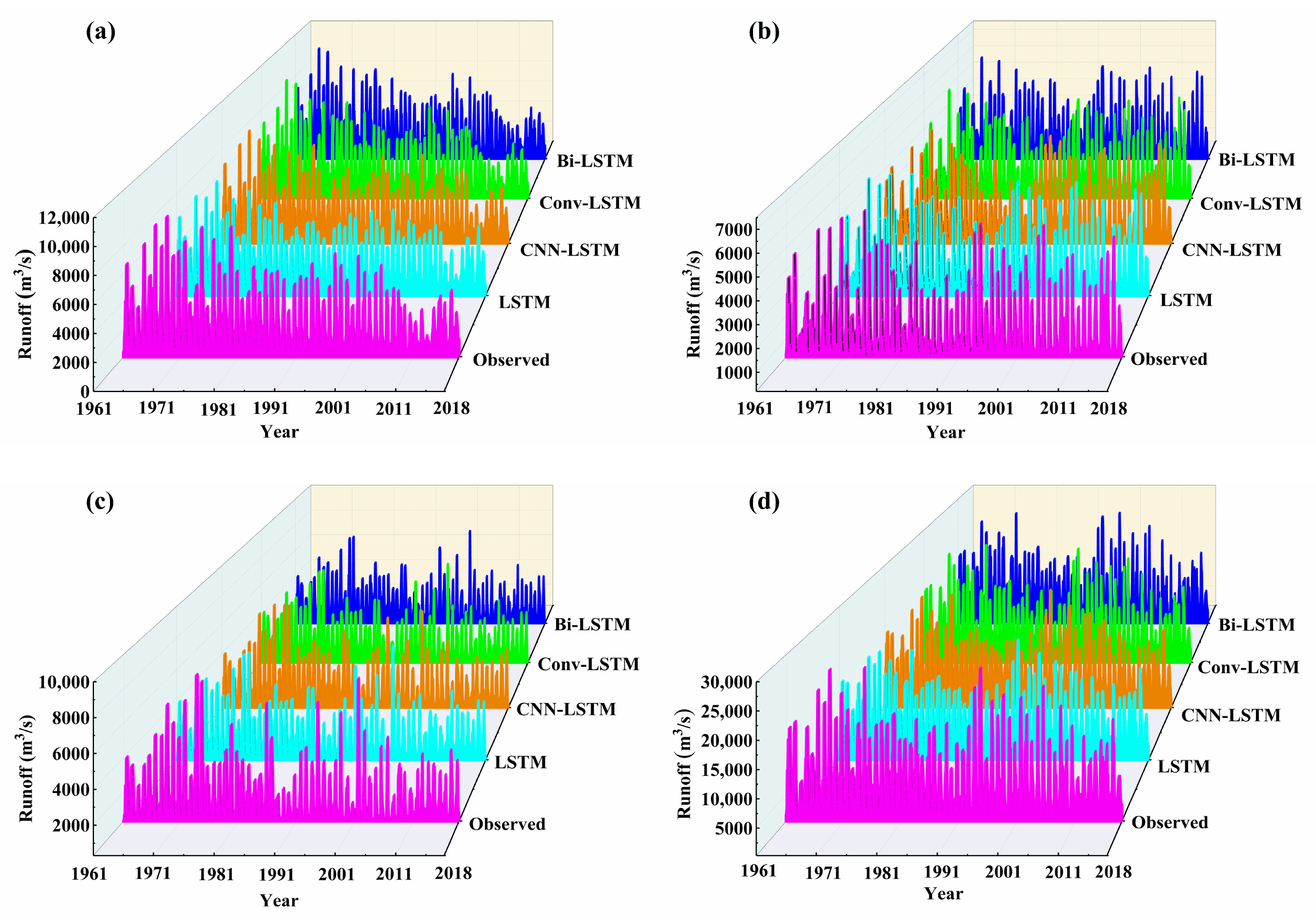
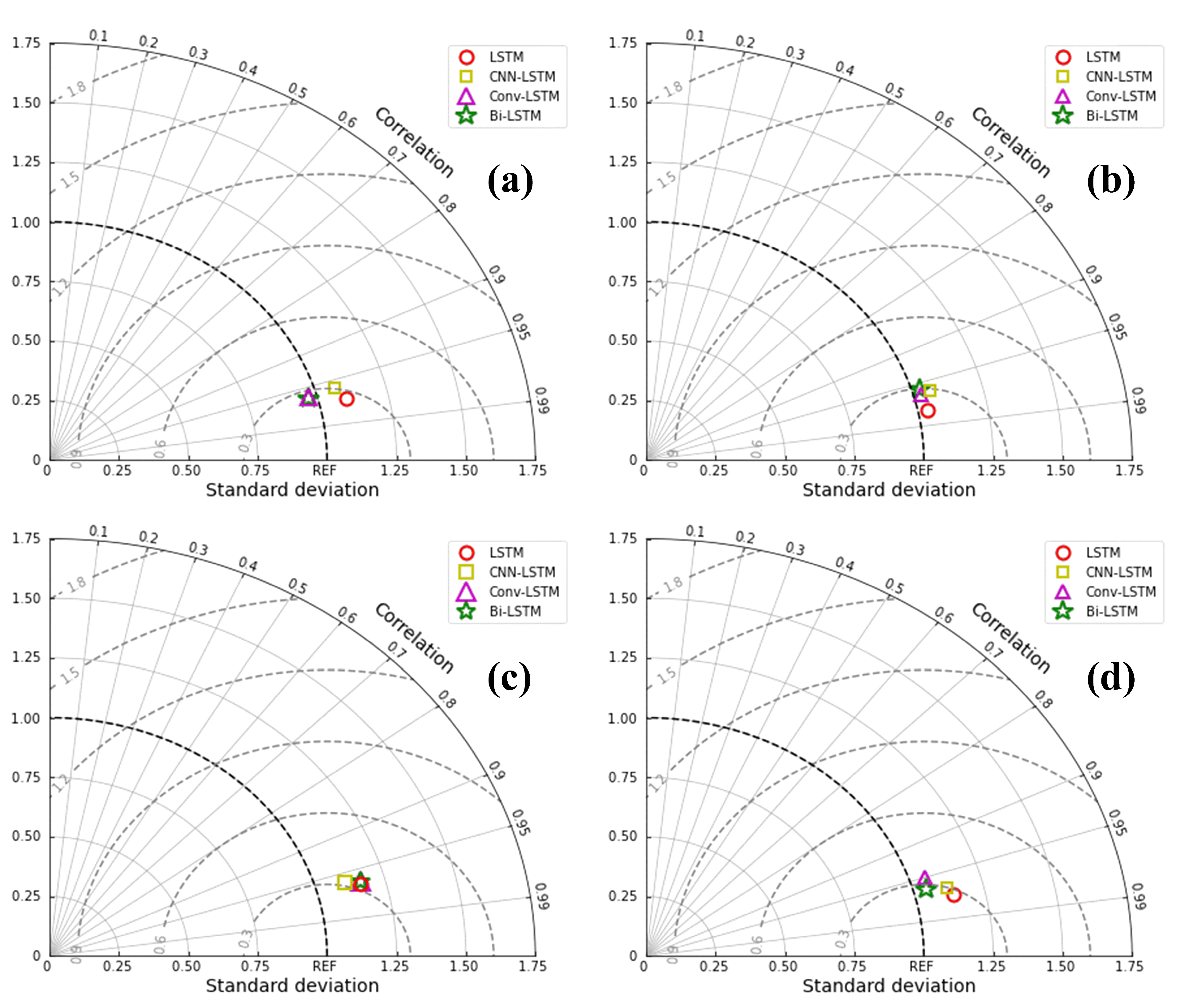
4.3.1. Prediction Performance of Different Models in the Same Forecast Period

To accurately study the predictive performance of different models within the same forecasting period, the historical runoff, precipitation, evaporation, and atmospheric circulation factors were selected as the input variables, and the predicted runoff was selected as the output variable. A 1-month time lag was used to capture the temporal variability. To avoid issues such as overfitting due to limited training data, monthly data from 1961 to 2010 were used as the training set, while data from 2011 to 2018 were used as the testing set for model training and evaluation. Figure 6 shows the runoff forecast results in the four stations of QJ, LZ, GG, and WZ in the XJB. It is worth noting that the predicted runoff in the four models closely matched the observed runoff, with a consistent overall trend of runoff variation. This indicated that the employed models had a high accuracy in predicting runoff, making them viable options for runoff forecasting.

Figure 7 compares the observed and predicted runoffs obtained from different models in WZ. It could be seen that all four models demonstrated relatively high accuracy. The LSTM model had the highest level of fit, with data points tightly clustered around the fitted line. The other three models (CNN-LSTM, Conv-LSTM, and Bi-LSTM) showed varying degrees of deviation from the fitted line. Overall, compared with the LSTM model, there were still some deviations in the prediction results from other models.

To better visualize the performance of different models in predicting runoff at various hydrological stations and address the issue where similar a distribution cannot be inferred from images, several evaluation metrics were introduced to quantitatively assess the prediction results (

Table 3. Evaluation index values of different models at different stations.

Station	Model	Training Set			Test Set
		NSE	RMSE (103 m3/s)	MAE (103 m3/s)	NSE	RMSE (103 m3/s)	MAE (103 m3/s)
QJ	LSTM	0.944	0.456	0.274	0.950	0.249	0.203
	CNN-LSTM	0.921	0.529	0.308	0.920	0.305	0.244
	Conv-LSTM	0.920	0.535	0.312	0.939	0.275	0.218
	Bi-LSTM	0.927	0.526	0.296	0.942	0.269	0.212
LZ	LSTM	0.959	0.252	0.137	0.960	0.241	0.210
	CNN-LSTM	0.925	0.338	0.163	0.926	0.343	0.282
	Conv-LSTM	0.929	0.337	0.231	0.925	0.363	0.326
	Bi-LSTM	0.916	0.362	0.251	0.926	0.340	0.269
GG	LSTM	0.933	0.405	0.237	0.954	0.221	0.195
	CNN-LSTM	0.922	0.416	0.248	0.923	0.286	0.242
	Conv-LSTM	0.927	0.415	0.246	0.919	0.296	0.249
	Bi-LSTM	0.928	0.412	0.242	0.922	0.288	0.245
WZ	LSTM	0.950	1.318	0.869	0.955	0.833	0.698
	CNN-LSTM	0.934	1.439	0.901	0.923	1.060	0.818
	Conv-LSTM	0.900	1.695	0.928	0.906	1.197	0.922
	Bi-LSTM	0.920	1.460	0.916	0.911	1.153	0.867

). It was observed that the LSTM model achieved the highest training accuracy among the four stations in the training dataset, with NSE values ranging from 0.933 to 0.959, RMSE values ranging from 0.252 to 1.318 (10³ m³/s), and MAE values ranging from 0.137 to 0.869 (10³ m³/s). Moreover, the LSTM model exhibited superior predictive performance in the testing dataset as well, with NSE ranging from 0.950 to 0.960, RMSE ranging from 0.221 to 0.833 (10³ m³/s), and MAE ranging from 0.195 to 0.698 (10³ m³/s). The NSE value of the CNN-LSTM model was approximately 0.92 across all four stations, and the Conv-LSTM and Bi-LSTM models exhibited an NSE value of approximately 0.91 in GG and WZ. Furthermore, the NSE value remained steady at around 0.93 in QJ and LZ. It could be concluded that although the Conv-LSTM and Bi-LSTM models had good generalization ability, their predictive performance was affected by station data, and their prediction accuracy at different stations had greater uncertainty compared to that of the LSTM and CNN-LSTM models. In addition, due to the differences in the actual runoff at different stations, RMSE and MAE exhibited varying patterns. Among them, the RMSE and MAE values in WZ were significantly larger than those at the other three stations, which was because the WZ station was located downstream of the XJB and to some extent aggregates the runoff from the other three upstream stations.

In order to enrich the evaluation criteria for different models, Taylor diagrams were introduced to assess their predictive performance. Firstly, the standard deviation was normalized to eliminate the problem of varying station data causing differences in magnitude (Figure 8 and Figure 9). Based on Figure 8, it was observed that the correlation coefficients between the predicted and observed runoff values of different models within the training dataset were consistently above 0.95, which suggested that the prediction results made by the four models were reliable. Furthermore, taking into account the varying representative locations of these models across differing stations, it was found that LSTM exhibited the highest correlation, followed by the CNN-LSTM, Bi-LSTM, and Conv-LSTM models. As seen in Figure 9, it was evident that the test set exhibited a higher degree of correlation compared to the training set, which suggested that the model had undergone significant improvements in accuracy after being trained. Through the above analysis, it can be inferred that among the four hydrological stations in the XJB, the LSTM model outperformed the other three models in terms of both accuracy and reliability. Moreover, the predicted results generated by the LSTM model also exhibited the highest degree of correlation with the observed values.

4.3.2. Prediction Performance of Optimal Model under Different Foresight Periods

According to the previous analysis, it is known that the LSTM model has the highest accuracy in predicting runoff in the XJB, and the NSE can reach above 0.95 for a 1-month time lag. To investigate the prediction accuracy of the model under a different forecast period, the LSTM model was used to predict the monthly runoff with a forecast period of 1–3 months in the XJB (

Table 4. Comparison of prediction effect of LSTM model in test set under different foresight periods.

Forecast Period	Error Indicator	QJ	LZ	GG	WZ
1 month	NSE	0.950	0.960	0.954	0.955
	RMSE (103 m3/s)	0.249	0.241	0.221	0.833
	MAE (103 m3/s)	0.203	0.210	0.195	0.698
2 month	NSE	0.897	0.901	0.889	0.893
	RMSE (103 m3/s)	0.295	0.274	0.243	1.310
	MAE (103 m3/s)	0.266	0.280	0.244	0.832
3 month	NSE	0.858	0.863	0.859	0.849
	RMSE (103 m3/s)	0.312	0.290	0.269	1.664
	MAE (103 m3/s)	0.297	0.321	0.276	0.920

). In the QJ station, the NSE values for a forecast period of 1–3 months were 0.950, 0.897, and 0.858, respectively, with values decreasing by 5.58% and 4.35%, respectively. In the LZ Station, the NSE values for a forecast period of 1–3 months were 0.960, 0.901, and 0.863, with values decreasing by 6.15% and 4.22%, respectively. In the GG Station, the NSE values for a forecast period of 1–3 months were 0.954, 0.889, and 0.859, with values decreasing by 6.81% and 3.37%, respectively. In the WZ Station, the NSE values for a forecast period of 1–3 months were 0.955, 0.893, and 0.849, with values decreasing by 6.49% and 4.93%, respectively. It can be inferred from the above analysis that with the increase of the forecasting horizon, the accuracy of the model tends to decrease to some extent. Moreover, the decrease in accuracy was relatively smaller for a 3-month forecasting horizon than for a 2-month horizon. Additionally, the changing trends of the RMSE and MAE increased with the decrease in NSE.

4.4. Interpretability Analysis of LSTM Model

According to the predicted results in the models, it can be inferred that the optimal model was the LSTM. To improve the interpretability of this model, we utilized the SHAP visualization tool to investigate the importance and the positive and negative effects of each input feature on the predicted results. The mean SHAP values of each feature were calculated based on the average of the absolute SHAP values of all samples. The contribution degree and global impact of input features are shown in Figure 10 and Figure 11. The contribution degree of input features was generated based on the SHAP value, which sorts features according to their impact on model output. In this figure, the SHAP value of each feature represented its relative contribution to the model output. The global impact graph provided a more macro perspective, showing the overall impact of each feature in the model on the output. It did not just focus on the impact of a single sample but also revealed the model’s feature impact changes across the input space. In the input feature contribution, we could identify the features that had an important impact on the prediction and then understand why the model made a certain prediction. In a global impact graph, each data point represented a sample, and the variable points of a feature were arranged according to the size of the SHAP value. If there are multiple variable points with the same SHAP value, it means that these features had a similar degree of influence on the model’s prediction results. The number of variable points with the same SHAP value could reflect the common impact of features in the overall model, providing us with deeper insight and interpretation. As seen in Figure 10, it was evident that the influence of different input features on the runoff prediction results was consistent throughout the basin. Specifically, historical runoff had the greatest impact, followed by precipitation, and finally evaporation and NPI. Figure 11 showed that the historical runoff, precipitation, and NPI had varying degrees of positive impacts on the predicted runoff, with a positive correlation, while evaporation had a negative impact on the predicted runoff, with a negative correlation. In addition, due to the strong spatial heterogeneity within the XJB, the contributions of meteorological factors, such as precipitation and evaporation, to runoff generation varied among different sub-basins. The interpretation results were consistent with the actual law in a certain range, which can further enhance the credibility of the model.

5. Discussion

5.1. Reasons for Differences in Model Prediction Accuracy

The time scale of the runoff prediction (hour, day, month) should serve water resource management, such as water resource scheduling, water resource allocation, and flood and drought disaster prevention. The LSTM and its variant models used in this study, namely CNN-LSTM, Conv-LSTM, and Bi-LSTM, had achieved good prediction results in other basins and at different time scales [24,25,36,66,67,68,69]. In terms of data sets, the training set size allowed the models to be trained adequately. First, the training set was large enough in number to cover the diversity and complexity of the data, and the data set was taken from real data. In addition, from the results of model training, the index NSE of the training set and the test set of the LSTM model and its variant models in different hydrological stations could reach above 0.90, and there was little difference between the two values. Among them, the LSTM model with the best accuracy can reach the maximum of 0.960 in the test set of the LZ station. The models could achieve excellent performance, and there was no overfitting or underfitting phenomenon, with a certain generalization ability. In terms of selecting input variables, historical runoff, precipitation, evaporation data, and atmospheric circulation factors were chosen as input variables for the models. The parameters of each model are fully calibrated to achieve the corresponding highest accuracy. The predictive performances of different models were analyzed, and the results showed that the LSTM model had a higher prediction accuracy and stability than other variant models across different stations in the XJB (as shown in Table 3). The possible reasons for the difference in predictive accuracy among different models are that the CNN-LSTM, Conv-LSTM, and Bi-LSTM models have made improvements based on the LSTM model, enhancing their abilities in different aspects. However, this enhancement of ability also has limitations. As for the aforementioned variant models, the CNN-LSTM model is mainly used in image processing. In the case of processing different types of data, it requires a conversion of data format, which limits its ability to perform direct processing [70]. When processing temporal information, the Conv-LSTM model is parallelly stacked in layers, and each layer operates independently. However, extracting spatial features may affect the propagation of temporal information, resulting in a decrease in its ability to process temporal information and subsequently leading to a decrease in its predictive accuracy [71]. The Bi-LSTM model still cannot transmit the starting point information of a sequence well for excessively long sequences. In the case of streamflow prediction, when dealing with a large quantity of data over a long period of time, this limitation results in its relatively low predictive accuracy [72].

5.2. Uncertainty

There are two main sources of uncertainty in this study. Firstly, there are missing data for certain months from the period of 1988–2000 in the LZ station. Although these gaps were filled using downstream station data and underwent rigorous quality control, the interpolated values may not be completely accurate, which could potentially affect the model training and prediction results. Secondly, the selection of model parameters directly affects the prediction results. In this study, the parameters were selected using a controlled variable approach, and the chosen parameters were within the optimal range. However, it is unknown whether there are better parameters outside of this range.

5.3. Advantages and Limitations

Global climate change has led to increasingly unpredictable weather patterns, including frequent occurrences of extreme flood and drought events, which has brought about more uncertainty in the prediction of river runoffs. In addition, the accuracy of forecasts is influenced by uncertain factors such as model structure and input variables. Therefore, it is crucial to select a suitable set of forecast factors from numerous hydro-meteorological elements for a given watershed [53,73,74]. In this study, the selection of forecast factors was primarily based on two considerations. Firstly, early-stage runoff was taken into account due to its strong autocorrelation and the assumption that the historical patterns of a runoff would continue into the future [75]. Secondly, other factors that affect a runoff were also considered. From the perspective of the runoff generation mechanism, it is known that the formation process of runoff is mainly influenced by climate factors and underlying surface conditions in the watershed. Among these factors, climate characteristics, particularly precipitation and evaporation, are the most important factors that affect long-term runoff changes [76]. Precipitation is the source of runoffs, and its spatial distribution and amount directly affect the formation of runoffs. Additionally, the magnitude of evaporation affects variations in the amount of runoff [77]. Moreover, the XJB is located in a monsoon precipitation zone where atmospheric circulation factors have a certain influence on climate change [78]. Yang et al. indicate that the NPI has a significant influence on the runoff change in the basin, which supports our research results [79]. Understanding the predictions made by deep learning models is currently a challenge in the field of machine learning. Previous studies have mostly failed to explain the reasons behind the model’s predicted results [80]. In this study, we use a game theory-based global sensitivity analysis method called the SHAP interpretability method to analyze the contribution of each input feature to the predicted results, and thus improve the reliability and application value of the model. Figure 10 and Figure 11 demonstrate that historical runoff has the greatest impact on runoff prediction, followed by precipitation, evaporation, and NPI, respectively.

This paper proposes the application of LSTM and its variant models in runoff prediction for the XJB. The aim is to provide decision-makers with a convenient and reliable method for accurate runoff predictions with high predictive accuracy. However, there are also some limitations in this paper. The hydrological stations selected in this study are mainly located in the middle and lower reaches of the XJB, and further verification of the applicability of the model to the entire XJB requires additional hydrological stations.

6. Conclusions

Based on precipitation, runoff, and other data from the XJB from 1961 to 2018, this paper constructed a runoff prediction model using LSTM and its variant models. Historical runoff, precipitation, evaporation, and the NPI (an atmospheric circulation factor) were used as inputs, while the predicted runoff was the output. The optimal model was chosen based on a comparison of predicted and observed values. The selected optimal model was then used to analyze the runoff predictions for different foresight periods. In addition, the SHAP method was employed to analyze the interpretability of the optimal model, identifying the importance and contribution (positive or negative) of each input feature to the predicted results. The findings are summarized below:

(1)

The NPI is the most influential atmospheric circulation factor affecting the runoff in the XJB.

(2)

When comparing different models with the same forecast period, the LSTM model had higher NSE results in the QJ, LZ, GG, and WZ, with values of 0.950, 0.960, 0.954, and 0.955, respectively. These values were higher than those in the other three models tested at the same stations. Therefore, it can be concluded that the LSTM model is the optimal choice among the four models used in this study.

(3)

With the optimal model, the LSTM model, its prediction results decreased as the foresight period increased. Specifically, the NSE decreased by 4.7% when the foresight period increased from one month to two months, and it decreased by 3.9% when the foresight period increased from two months to three months. This suggested that although the decrease in the NSE was slow as the foresight period increased, there was a converging trend of a declining NSE with a longer foresight period.

(4)

Based on SHAP values, an interpretability analysis was conducted on the LSTM model. The results showed that in the XJB, historical runoff had the greatest impact on runoff prediction results, followed by precipitation, evaporation, and the NPI. Evaporation was negatively correlated with runoff, while historical runoff, precipitation, and the NPI were positively correlated.

References

1. Dey, P.; Mishra, A. Separating the impacts of climate change and human activities on streamflow: A review of methodologies and critical assumptions. J. Hydrol. 2017, 548, 278–290. [Google Scholar] [CrossRef]
2. Sepehri, A.; Sarrafzadeh, M.H. Effect of nitrifiers community on fouling mitigation and nitrification efficiency in a membrane bioreactor. Chem. Eng. Process. 2018, 128, 10–18. [Google Scholar] [CrossRef]
3. Zhang, S.; Chen, J.; Gu, L. Overall uncertainty of climate change impacts on watershed hydrology in China. Int. J. Climatol. 2022, 42, 507–520. [Google Scholar] [CrossRef]
4. Zhu, S.; Zhou, J.Z.; Ye, L.; Meng, C.Q. Streamflow estimation by support vector machine coupled with different methods of time series decomposition in the upper reaches of Yangtze River, China. Environ. Earth Sci. 2016, 75, 531. [Google Scholar] [CrossRef]
5. Amiri, E. Forecasting daily river flows using nonlinear time series models. J. Hydrol. 2015, 527, 1054–1072. [Google Scholar] [CrossRef]
6. Speight, L.J.; Cranston, M.D.; White, C.J.; Kelly, L. Operational and emerging capabilities for surface water flood forecasting. Wires Water 2021, 8, e1517. [Google Scholar] [CrossRef]
7. Kalra, A.; Miller, W.P.; Lamb, K.W.; Ahmad, S.; Piechota, T. Using large-scale climatic patterns for improving long lead time streamffow forecasts for Gunnison and San Juan River Basins. Hydrol. Process. 2013, 27, 1543–1559. [Google Scholar] [CrossRef]
8. Lin, G.F.; Chou, Y.C.; Wu, M.C. Typhoon flood forecasting using integrated two-stage Support Vector Machine approach. J. Hydrol. 2013, 486, 334–342. [Google Scholar] [CrossRef]
9. Xu, X.; Yang, D.; Yang, H.; Lei, H. Attribution analysis based on the Budyko hypothesis for detecting the dominant cause of runoff decline in Haihe basin. J. Hydrol. 2014, 510, 530–540. [Google Scholar] [CrossRef]
10. Faghih, M.; Mirzaei, M.; Adamowski, J.; Lee, J.; El-Shaffe, A. Uncertainty estimation in ffood inundation mapping: An application of non-parametric bootstrapping: Uncertainty in ffood inundation mapping. River Res. Appl. 2017, 33, 611–619. [Google Scholar] [CrossRef]
11. Van, S.P.; Le, H.M.; Thanh, D.V.; Dang, T.D.; Loc, H.H.; Anh, D.T. Deep learning convolutional neural network in rainfall–runoff modelling. J. Hydroinformatics 2020, 22, 541–561. [Google Scholar] [CrossRef]
12. Dou, Y.; Ye, L.; Gupta, H.V.; Zhang, H.; Behrangi, A.; Zhou, H. Improved flood forecasting in basins with no precipitation stations: Constrained runoff correction using multiple satellite precipitation products. Water Resour. Res. 2021, 57, e2021WR029682. [Google Scholar] [CrossRef]
13. Kratzert, F.; Klotz, D.; Herrnegger, M.; Sampson, A.K.; Hochreiter, S.; Nearing, G.S. Toward improved predictions in ungauged basins: Exploiting the power of machine learning. Water Resour. Res. 2019, 55, 11344–11354. [Google Scholar] [CrossRef]
14. Mirzaei, M.; Yu, H.; Dehghani, A.; Galavi, H.; Shokri, V. A novel stacked long short-term memory approach of deep learning for streamflow simulation. Sustainability 2021, 13, 13384. [Google Scholar] [CrossRef]
15. Kim, T.; Yang, T.T.; Gao, S.; Zhang, L.J.; Ding, Z.Y.; Wen, X.; Gourley, J.J.; Hong, Y. Can artificial intelligence and data-driven machine learning models match or even replace process-driven hydrologic models for streamflow simulation?: A case study of four watersheds with different hydro-climatic regions across the CONUS. J. Hydrol. 2021, 598, 126423. [Google Scholar] [CrossRef]
16. Rahmani, F.; Lawson, K.; Ouyang, W.; Appling, A.; Oliver, S.; Shen, C. Exploring the exceptional performance of a deep learning stream temperature model and the value of streamflow data. Environ. Res. Lett. 2021, 16, 024025. [Google Scholar] [CrossRef]
17. Jiang, S.J.; Zheng, Y.; Solomatine, D. Improving AI system awareness of geoscience knowledge: Symbiotic integration of physical approaches and deep learning. Geophys. Res. Lett. 2020, 47, e2020GL088229. [Google Scholar] [CrossRef]
18. Fung, K.F.; Huang, Y.F.; Chai, H.K.; Mirzaei, M. Improved SVR machine learning models for agricultural drought prediction at downstream of Langat River Basin, Malaysia. J. Water Clim. Chang. 2020, 11, 1383–1398. [Google Scholar] [CrossRef]
19. Fan, C.; Song, C.; Liu, K.; Ke, L.; Xue, B.; Chen, T.; Fu, C.; Cheng, J. Century-scale reconstruction of water storage changes of the largest lake in the inner mongolia plateau using a machine learning approach. Water Resour. Res. 2021, 57, e2020WR028831. [Google Scholar] [CrossRef]
20. Karthikeyan, L.; Mishra, A.K. Multi-layer high-resolution soil moisture estimation using machine learning over the United States. Remote Sens. Environ. 2021, 266, 112706. [Google Scholar] [CrossRef]
21. Hochreiter, S.; Schmidhuber, J. Long short-term memory. Neural Comput. 1997, 9, 1735–1780. [Google Scholar] [CrossRef] [PubMed]
22. Liu, P.; Wang, J.; Sangaiah, A.; Xie, Y.; Yin, X.C. Analysis and prediction of water quality using LSTM deep neural networks in IoT environment. Sustainability 2019, 11, 2058. [Google Scholar] [CrossRef]
23. Gao, S.; Huang, Y.F.; Zhang, S.; Han, J.C.; Wang, G.Q.; Zhang, M.X.; Lin, Q.A. Short-term runoff prediction with GRU and LSTM networks without requiring time step optimization during sample generation. J. Hydrol. 2020, 589, 125188. [Google Scholar] [CrossRef]
24. Gauch, M.; Kratzert, F.; Klotz, D.; Nering, G.; Lin, J.; Hochreiter, S. Rainfall-runoff prediction at multiple timescales with a single Long Short-Term Memory network. Hydrol. Earth Syst. Sci. 2021, 25, 2045–2062. [Google Scholar] [CrossRef]
25. Kratzert, F.; Klotz, D.; Brenner, C.; Schulz, K.; Herrnegger, M. Rainfall–runoff modelling using long short-term memory (LSTM) networks. Hydrol. Earth Syst. Sci. 2018, 22, 6005–6022. [Google Scholar] [CrossRef]
26. Yuan, X.H.; Chen, C.; Lei, X.H.; Yuan, Y.B.; Adnan, R.M. Monthly runoff forecasting based on LSTM–ALO model. Stoch. Environ. Res. Risk Assess. 2018, 32, 2199–2212. [Google Scholar] [CrossRef]
27. Le, X.H.; Ho, H.V.; Lee, G.; Jung, S. Application of long short-term memory (LSTM) neural network for flood forecasting. Water 2019, 11, 1387. [Google Scholar] [CrossRef]
28. Kao, I.F.; Zhou, Y.L.; Chang, L.C.; Chang, F.J. Exploring a Long Short-Term Memory based Encoder-Decoder framework for multi-step-ahead flood forecasting. J. Hydrol. 2020, 583, 124631. [Google Scholar] [CrossRef]
29. Zhang, J.Y.; Yan, H. A long short-term components neural network model with data augmentation for daily runoff forecasting. J. Hydrol. 2023, 617, 128853. [Google Scholar] [CrossRef]
30. Kim, T.Y.; Cho, S.B. Predicting residential energy consumption using CNN-LSTM neural networks. Energy 2019, 182, 72–81. [Google Scholar] [CrossRef]
31. Huang, C.J.; Kuo, P.H. A deep cnn-lstm model for particulate matter (PM2.5) forecasting in smart cities. Sensors 2018, 18, 2220. [Google Scholar] [CrossRef]
32. Barzegar, R.; Aalami, M.T.; Adamowski, J. Short-term water quality variable prediction using a hybrid CNN-LSTM deep learning mode. Stoch. Stoch. Environ. Res. Risk Assess. 2020, 34, 415–433. [Google Scholar] [CrossRef]
33. Moishin, M.; Deo, R.C.; Prasad, R.; Raj, N.; Abdulla, S. Designing deep-based learning flood forecast model with ConvLSTM hybrid algorithm. IEEE Access 2021, 9, 50982–50993. [Google Scholar] [CrossRef]
34. Barzegar, R.; Aalami, M.T.; Adamowski, J. Coupling a hybrid CNN-LSTM deep learning model with a boundary corrected maximal overlap discrete wavelet transform for multiscale Lake water level forecasting. J. Hydrol. 2021, 598, 126196. [Google Scholar] [CrossRef]
35. Jaseena, K.U.; Kovoor, B.C. Decomposition-based hybrid wind speed forecasting model using deep bidirectional LSTM networks. Energ. Convers. Manag. 2021, 234, 113944. [Google Scholar] [CrossRef]
36. Ha, S.; Liu, D.; Mu, L. Prediction of Yangtze River streamflow based on deep learning neural network with El Niño-Southern Oscillation. Sci. Rep. 2021, 11, 11738. [Google Scholar] [CrossRef] [PubMed]
37. Montavon, G.; Samek, W.; Müller, K.R. Methods for interpreting and understanding deep neural networks. Digit. Signal Process. 2018, 73, 1–15. [Google Scholar] [CrossRef]
38. McGovern, A.; Ryan, L.; Gagne, D.J.; Jergensen, G.E.; Elmore, K.L.; Homeyer, C.R.; Smith, T. Making the black box more transparent: Understanding the physical implications of machine learning. Bull. Am. Meteorol. Soc. 2019, 100, 2175–2199. [Google Scholar] [CrossRef]
39. Nearing, G.S.; Kratzert, F.; Sampson, A.K.; Pelissier, C.S.; Klotz, D.; Frame, J.M.; Prieto, C.; Gupta, H.V. What role does hydrological science play in the age of machine learning? Water Resour. Res. 2020, 57, e2020WR028091. [Google Scholar] [CrossRef]
40. Lee, Y.G.; Oh, J.Y.; Kim, D.; Kim, G. Shap value-based feature importance analysis for short-term load forecasting. J. Electr. Eng. Technol. 2023, 18, 579–588. [Google Scholar] [CrossRef]
41. Kitani, R.; Iwata, S. Verification of Interpretability of Phase-Resolved Partial Discharge Using a CNN With SHAP. IEEE Access 2023, 11, 4752–4762. [Google Scholar] [CrossRef]
42. Linardatos, P.; Papastefanopoulos, V.; Kotsiantis, S. Explainable ai: A review of machine learning interpretability methods. Entropy 2020, 23, 18. [Google Scholar] [CrossRef]
43. Xia, Q.; He, J.; He, B.; Chu, Y.; Li, W.; Sun, J.; Wen, D. Effect and genesis of soil nitrogen loading and hydrogeological conditions on the distribution of shallow groundwater nitrogen pollution in the North China Plain. Water Res. 2023, 243, 120346. [Google Scholar] [CrossRef] [PubMed]
44. Molnar, C. Interpretable Machine Learning; Lulu Press: Morrisville, NC, USA, 2020. [Google Scholar]
45. Štrumbelj, E.; Kononenko, I. Explaining prediction models and individual predictions with feature contributions. Knowl. Inf. Syst. 2014, 41, 647–665. [Google Scholar] [CrossRef]
46. Lundberg, S.M.; Lee, S.I. A unified approach to interpreting model predictions. Adv. Neural Inf. Process. Syst. 2017, 30, 4768–4777. [Google Scholar]
47. Lama, L.; Wilhelmsson, O.; Norlander, E.; Gustafsson, L.; Lager, A.; Tynelius, P.; Ẅarvik, L.; Östenson, C.G. Machine learning for prediction of diabetes risk in middle-aged Swedish people. Heliyon 2021, 7, e07419. [Google Scholar] [CrossRef] [PubMed]
48. Wen, X.; Xie, Y.; Wu, L.; Jiang, L. Quantifying and comparing the effects of key risk factors on various types of roadway segment crashes with LightGBM and SHAP. Accid. Anal. Prev. 2021, 159, 106261. [Google Scholar] [CrossRef]
49. Mangalathu, S.; Hwang, S.H.; Jeon, J.S. Failure mode and effects analysis of RC members based on machine-learning-based SHapley Additive exPlanations (SHAP) approach. Eng. Struct. 2020, 219, 110927. [Google Scholar] [CrossRef]
50. Wang, R.Z.; Kim, J.H.; Li, M.H. Predicting stream water quality under different urban development pattern scenarios with an interpretable machine learning approach. Sci. Total Environ. 2021, 761, 144057. [Google Scholar] [CrossRef]
51. Wang, S.; Peng, H.; Liang, S. Prediction of estuarine water quality using interpretable machine learning approach. J. Hydrol. 2022, 605, 127320. [Google Scholar] [CrossRef]
52. Huang, S.Z.; Li, P.; Huang, Q.; Leng, G.Y.; Hou, B.B.; Ma, L. The propagation from meteorological to hydrological drought and its potential influence factors. J. Hydrol. 2017, 547, 184–195. [Google Scholar] [CrossRef]
53. Liu, S.Y.; Huang, S.Z.; Huang, Q.; Xie, Y.Y.; Leng, G.Y.; Luan, J.K.; Song, X.Y.; Wei, X.; Li, X.Y. Identification of the non-stationarity of extreme precipitation events and correlations with large-scale ocean-atmospheric circulation patterns: A case study in the Wei River Basin, China. J. Hydrol. 2017, 548, 184–195. [Google Scholar] [CrossRef]
54. Meng, E.; Huang, S.; Huang, Q.; Fang, W.; Wang, H.; Leng, G.; Wang, L.; Liang, H. A hybrid VMD-SVM model for practical streamflow prediction using an innovative input selection framework. Water Resour. Manag. 2021, 35, 1321–1337. [Google Scholar] [CrossRef]
55. Song, P.; Liu, W.; Sun, J.; Wang, C.; Kong, L.; Nong, Z.; Lei, X.; Wang, H. Annual runoff forecasting based on multi-model information fusion and residual error correction in the Ganjiang River Basin. Water 2020, 12, 2086. [Google Scholar] [CrossRef]
56. Yan, X.G.; Wu, L.N.; Zhou, Y.; Song, J.L.; Deng, S.X. On the association of Co-kriging interpolation method research based on GlS: A case study in Karst area of Guizhou Province. J. Yunnan Univ. 2017, 39, 432–439. (In Chinese) [Google Scholar]
57. Khan, M.; Almazah, M.M.; EIlahi, A.; Niaz, R.; Al-Rezami, A.Y.; Zaman, B. Spatial interpolation of water quality index based on Ordinary kriging and Universal kriging. Geomat. Nat. Hazards Risk 2023, 14, 2190853. [Google Scholar] [CrossRef]
58. Wu, H.C.; Yang, Q.L.; Liu, J.M.; Wang, G.Q. A spatiotemporal deep fusion model for merging satellite and gauge precipitation in China. J. Hydrol. 2020, 584, 124664. [Google Scholar] [CrossRef]
59. Shi, X.; Gao, Z.; Lausen, L.; Wang, H.; Yeung, D.Y.; Wong, W.K.; Woo, W.C. Deep learning for precipitation nowcasting: A benchmark and a new model. Adv. Neural Inf. Process. Syst. 2017, 30, 144–146. [Google Scholar]
60. Wallace, J.M.; Gutzler, D.S. Teleconnections in the geopotential height field during the northern hemisphere winter. Bull. Am. Meteorol. Soc. 1981, 109, 784–812. [Google Scholar] [CrossRef]
61. Ng, E.K.W.; Chan, J.C.L. Geophysical applications of partial wavelet coherence and multiple wavelet coherence. J. Atmos. Ocean. Technol. 2012, 29, 1845–1853. [Google Scholar] [CrossRef]
62. Hu, W.; Si, B.C. Technical Note: Multiple wavelet coherence for untangling scale specific and localized multivariate relationships in geosciences. Hydrol. Earth Syst. Sci. 2016, 20, 3183–3191. [Google Scholar] [CrossRef]
63. Nalley, D.; Adamowski, J.; Biswas, A.; Gharabaghi, B.; Hu, W. A multiscale and multivariate analysis of precipitation and streamflow variability in relation to ENSO, NAO and PDO. J. Hydrol. 2019, 574, 288–307. [Google Scholar] [CrossRef]
64. Nash, J.E.; Sutcliffe, J.V. River flow forecasting through conceptual models part I-A discussion of principles. J. Hydrol. 1970, 10, 282–290. [Google Scholar] [CrossRef]
65. Yu, D.Y.; Zhu, W.J.; Pan, Y.Z. The role of atmospheric circulation system playing in coupling relationship between spring NPP and precipitation in East Asia area. Environ. Monit. Assess. 2008, 145, 135–143. [Google Scholar]
66. Sangrody, H.; Zhou, N.; Salih, T.; Khorramdel, B.; Motalleb, M.; Sareiloo, M. Long term forecasting using machine learning methods. In Proceedings of the IEEE Power and Energy Conference at Illinois (PECI), Champaign, IL, USA, 22–23 February 2018; IEEE: Piscataway, NJ, USA, 2018; pp. 1–5. [Google Scholar]
67. Yue, Z.X.; Ai, P.; Xiong, C.S.; Hong, M.; Song, Y.H. Mid- to long-term runoff prediction by combining the deep belief network and partial least-squares regression. J. Hydroinformatics 2020, 22, 1283–1305. [Google Scholar] [CrossRef]
68. Li, P.; Zhang, J.; Krebs, P. Prediction of flow based on a CNN-LSTM combined deep learning approach. Water 2022, 14, 993. [Google Scholar] [CrossRef]
69. Wu, J.H.; Wang, Z.C.; Hu, Y.; Tao, S.; Dong, J.H.; Tsakiris, G. Runoff forecasting using convolutional neural networks and optimized Bi-directional long short-term memory. Water Resour. Manag. 2023, 37, 937–953. [Google Scholar] [CrossRef]
70. Gamboa, J.C.B. Deep Learning for time-series analysis. Comput. Sci. 2017, 1701, 01887. [Google Scholar]
71. Wang, Y.; Long, M.; Wang, J.; Gao, Z.; Yu, P.S. PredRNN: Recurrent neural networks for predictive learning using spatiotemporal LSTMs. Adv. Neural Inf. Process. Syst. 2017, 30, 1–10. [Google Scholar]
72. Wang, S.Z.; Cao, J.N.; Yu, P. Deep Learning for spatio-temporal data mining: A survey. IEEE Trans. Knowl. Data Eng. 2022, 34, 3681–3700. [Google Scholar] [CrossRef]
73. Sivakumar, B.; Berndtsson, R. Advances in Data-Based Approaches for Hydrologic Modeling and Forecasting; World Scientific: Singapore, 2010. [Google Scholar]
74. Bai, Y.; Bezak, N.; Zeng, B.; Li, C.; Zhang, J. Daily runoff forecasting using a cascade long short-term memory model that considers different variables. Water Resour. Manag. 2021, 35, 1167–1181. [Google Scholar] [CrossRef]
75. Zeng, M.; Li, J.Q.; Ming, Y.W.; Yang, S.S.; Li, J. Analysis on the influence of reservoir group on the runoff of Datong station in dry season. IOP Conf. Ser. Earth Environ. Sci. 2021, 768, 012047. [Google Scholar] [CrossRef]
76. Guo, W.X.; Hu, J.W.; Wang, H.X. Analysis of runoff variation characteristics and influencing factors in the Wujiang River basin in the past 30 years. Int. J. Environ. Res. Public Health 2021, 19, 372. [Google Scholar] [CrossRef] [PubMed]
77. Jong, S.I.; Om, K.C.; Pak, Y.I. Influences of atmospheric circulation patterns on interannual variability of winter precipitation over the northern part of the Korean Peninsula. Clim. Res. 2021, 85, 35–50. [Google Scholar] [CrossRef]
78. Zhang, Q.; Xiao, M.; Singh, V.P.; Li, J. Regionalization and spatial changing properties of droughts across the Pearl River basin, China. J. Hydrol. 2012, 472, 355–366. [Google Scholar] [CrossRef]
79. Yang, P.; Zhang, S.; Xia, J.; Zhan, C.; Wang, W.; Luo, X.; Chen, N.; Li, J. Analysis of drought and flood alternation and its driving factors in the Yangtze River basin under climate change. Atmos. Res. 2022, 270, 106087. [Google Scholar] [CrossRef]
80. Simonyan, K.; Zisserman, A. Very deep convolutional networks for large-scale image recognition. Comput. Sci. 2014, 9, 1556. [Google Scholar]
Figure 1. Location of the XJB and selected hydrologic control stations and meteorological stations.
Water 15 03184 g001
Figure 2. The schematic diagrams of different models: (a) LSTM, (b) CNN-LSTM, (c) Conv-LSTM, and (d) Bi-LSTM.
Water 15 03184 g002
Figure 3. Time-lag selection is based on the highest correlation coefficients, with HR, P, E, NPI, and PR denoting historical runoff, precipitation, evaporation, North Pacific Index, and predicted runoff, respectively.
Water 15 03184 g003
Figure 4. Cross-wavelet coherence spectrum (the arrow pointing to the right (left) indicates an in-phase (anti-phase) relationship between runoff and other factors. The area enclosed by the thick black solid line represents the region passing a 95% confidence test. The same below).
Water 15 03184 g004
Figure 5. Cross-wavelet energy spectrum between runoff and other factors.
Water 15 03184 g005
Figure 6. Comparison of observed and predicted runoff in the (a) QJ, (b) LZ, (c) GG, and (d) WZ stations, respectively.
Water 15 03184 g006
Figure 7. Comparison of observed and predicted runoffs based on the (a1,a2) LSTM, (b1,b2) CNN-LSTM, (c1,c2) Conv-LSTM, and (d1,d2) Bi-LSTM models, respectively.
Water 15 03184 g007
Figure 8. Taylor plots of training set in the (a) QJ, (b) LZ, (c) GG, and (d) WZ stations, respectively, with the horizontal and vertical coordinates representing standard deviation, the internal dashed line representing RMSE, the outer arc representing the correlation coefficient, and the same below.
Water 15 03184 g008
Figure 9. Taylor plots of test set in the (a) QJ, (b) LZ, (c) GG, and (d) WZ stations, respectively.
Water 15 03184 g009
Figure 10. Importance rankings of input features in the (a) QJ, (b) LZ, (c) GG, and (d) WZ stations, respectively.
Water 15 03184 g010
Figure 11. Global influence map of input features in the (a) QJ, (b) LZ, (c) GG, and (d) WZ stations, respectively. The positive values represent positive correlation and negative values represent negative correlation.
Water 15 03184 g011