Abstract
The study evaluated nine empirical methods for estimating reference evapotranspiration (ETo) in Bosnia and Herzegovina (BiH) across different climatic zones. The methods compared were the Hargreaves–Samani method (HS), the modified Hargreaves–Samani method (HM), the calibrated Hargreaves–Samani method (HC), the Priestley–Taylor method (PT), the Copais method (COP), the Makkink method (MAK), the Penman–Monteith method based on air temperature and overall average windspeed (PMT2), the Penman–Monteith method based on air temperature and regional average windspeed (PMT1.3), and the Penman–Monteith method based on air temperature and site-specific windspeed (PMTlok). These methods were tested against the “Food Agricultural Organization-Penman Monteith approach” (FAO-PM). The evaluation was performed using data from 20 meteorological stations in BiH, considering a common irrigation season (April–October) for two periods (2000–2005 and 2018–2022). The stations represented three climatic zones: semi-arid (SA), dry sub-humid (DSH), and moist sub-humid (MSH). The performance and ranking of the ETo methods were analyzed using the TOPSIS method. The trend of ETo during the common irrigation season for the period from 2018 to 2022 was determined using the Mann–Kendall test. The results of the study indicated that the HC method showed the best performance across all three climatic zones. The average root mean square error (RMSE) was 0.67 mm day−1, 0.49 mm day−1, and 0.50 mm day−1 for the SA, DSH, and MSH zones, respectively. As an alternative to the HC method, the PT method is recommended for its favorable results in both periods and in all zones. On the other hand, the HS method exhibited the highest average overestimation, particularly in the MSH zone, where ETo values were 18% higher compared with those of the FAO-PM method. The COP method also showed high overestimation and was not recommended for use. Regarding the MAK method, it resulted in underestimation during the period from 2000 to 2005, ranging from 17% in the DSH zone to 11% in the MSH zone. However, its performance improved during the period from 2018 to 2022, for which it ranked second place in the MSH zone. Among the PMT methods, the PMTlok, which utilized local average windspeed, yielded the best results. Despite performing well in the neighboring country of Serbia, the HM method showed poor overall performance in BiH. The findings of this study can serve as a foundation for further research in BiH to enhance irrigation practices in response to climate changes.
1. Introduction
Crop evapotranspiration (ETc) is a crucial factor in the planning and management of water resources in agriculture. Accurate estimation of ETc allows for efficient irrigation scheduling and optimal water use, leading to improved crop yield and water conservation. Evapotranspiration is defined as a physical process whereby water is transferred to the soil-plant-atmosphere system [1]. The ETc can be directly measured using the Eddy covariance method (EC) and a lysimeter and indirectly measured using the reference evapotranspiration (ETo) and crop coefficient (Kc). Direct measurement of ETo using the micrometeorological technique of Eddy covariance offers distinct advantages, relying on fewer theoretical assumptions and demonstrating broad applicability. This approach is highly valued by micrometeorologists, as it directly captures the exchange of gases and energy between ecosystems and the atmosphere. The Eddy covariance method precisely and continuously quantifies the fluxes in carbon and water vapor flows within an ecosystem, representing the most efficient means of gauging such exchanges [2]. Nevertheless, the significant cost associated with EC instruments and hardware can limit the number of observation points and hinder replication in sampling [3,4]. This cost limitation also introduces a significant bias in the global distribution of EC observations, which are primarily concentrated in Western Europe, the United States, and more recently, parts of Asia [4].
In contrast, weighing lysimeters offer an alternative for comprehensive quantification of various water sources including precipitation, dew, fog, and ETo itself. However, using lysimeters and processing real data introduces susceptibility to errors. These errors originate from factors such as data gaps, deviations due to external influences (e.g., animal contact), mass variations after leachate sampling, scale sensitivity to temperature changes, and crop growth and removal, among others [5]. Furthermore, lysimeters require significant volumes of soil to provide comparable heat and water transport conditions to undisturbed soil. They require unimpeded plant root growth, which requires extensive and expensive installation, especially for hydraulic weight lysimeters. Considering the significant maintenance and operational costs, especially in developing countries, various empirical methods have emerged to calculate ETo. Notably, the ETo and Kc approach is widely accepted for calculating crop evapotranspiration due to its simplicity and cost-effectiveness.
ETo represents the evapotranspirative power of the atmosphere under reference conditions, which are not influenced by specific crop characteristics or cultivation techniques. It is calculated based on weather parameters such as air temperature, relative humidity, wind speed, and solar radiation [1]. The crop coefficient (Kc) accounts for the crop-specific characteristics and growth stages, modifying the reference evapotranspiration to estimate the actual crop water requirement. Kc values are typically determined experimentally for different crop types and growth stages, and they are often updated and refined based on research and field observations [6,7].
The knowledge of ETo estimation is very important, primarily for the estimation of crop water requirements, soil–water balance, the use of hydrological models, as well as crop growth modeling. The ETo estimation models available in the literature [8,9] may be broadly classified as (1) fully physical combination models that account for mass and energy conservation principles; (2) semi-physical models that deal with either mass or energy conservation principles; and (3) black box models based on artificial neural networks, empirical relationships, and fuzzy and genetic algorithms.
In recent decades, an ETo revision has been performed, which has resulted in two standard procedures for ETo calculation. These assume that the surfaces underlying collected weather data are well watered, so that near-surface meteorological measurements reflect the cooling and humidifying effects of an evaporating surface. The two primary procedures are as follows:
- -
- The FAO (Food and Agriculture Organization), the FAO Expert Group on the Revision of Methods for Calculating Plant Water Requirements, which issued a publication called “FAO Irrigation and Drainage paper 56” and adopted grass as a reference crop.
- -
- The ASCE-EWRI (American Association of Civil Engineers—Institute for Water Resources and the Environment), the Committee for Standardization of Reference Evapotranspiration, which issued a report on standardized ETo and adopted alfalfa as a reference crop.
Both groups of scientists recommended the FAO Penman–Monteith (FAO-PM) method as the standard method for ETo calculation, as well as for testing the other ETo estimation methods [10]. The FAO-PM method is a new standard for reference evapotranspiration that overcomes the shortcomings of the previous FAO Penman method. It is based on a hypothetical crop with an assumed height of 0.12 m, a surface resistance of 70 s m−1, and an albedo of 0.23 [1]. This crop closely resembles the evaporation of an extension surface of green grass of uniform height, actively growing and adequately watered. The FAO-PM method provides values that are consistent with actual crop water use data worldwide [1].
The PM-ETo equation can be contradicted by researchers who would prefer not to have a standard evaporative surface with fixed characteristics such as grass, which are important when using lysimeters and other precise measurement systems [11]. The evaluation of vegetation conditions implies a precise assessment of the local plant cover, type, and density, which can differ significantly in various climate types. For instance, in arid and semi-arid regions, the vegetation may consist of drought-tolerant plants with sparse foliage, whereas in humid climates, lush and dense vegetation predominates. This divergence underscores the need for a nuanced approach that accommodates the specificities of each climate type. Water stress, together with degree of ground cover, can create an impact on the canopy resistance and albedo of green grass, induced by a high temperature and low air humidity [12,13,14,15]. In scenarios characterized by drought-induced water stress, the selection of a simplified empirical calculation for ETo becomes pivotal. Recent research highlights the standardized precipitation-evapotranspiration index (SPEI) as a multi-timescale indicator incorporating both precipitation and evapotranspiration [16]. The SPEI offers advanced insights into various types of droughts and their impacts on diverse climatic systems. Notably, several studies indicate that the SPEI index is particularly sensitive to the potential evapotranspiration variable within the SPEI assessment [17]. Consequently, the severity of drought events detected using the SPEI varies based on the accuracy of the chosen evapotranspiration method [16,18].
However, the FAO-PM method is not without limitations. The main disadvantage of the FAO-PM method is the need for numerous input data, which are often not available at meteorological sites [19,20,21], especially in developing countries such as Bosnia and Herzegovina (BiH) [19] or other regions [22]. When the data are available, they are often inaccurate due to poor maintenance of meteorological sites and sensors, especially those for solar radiation, humidity, and windspeed measurement [23]. The problem with the windspeed measurements is usually due to inadequate fetch around the sensors, whereas imperfections in humidity data might be due to the inadequate aeration of the shelter in which the sensor is placed. Other problems might be due to advection, especially in dry areas. In some cases, the FAO-PM method tends to underestimate ETo in semi-arid and windy regions (2–18%) compared to the measured ETo values [24,25]. ETo underestimation by the FAO-PM method might be also due to the fixed value of surface resistance (rs) [26,27].
The above text highlights the challenges associated with estimating reference evapotranspiration (ETo) in BiH due to limited data availability. These limitations lead to the development and use of empirical methods that require less input parameters for ETo calculation. Among numerous empirical methods, the most attention has been given to those that require only air temperature data, since this parameter is widely available at meteorological stations, and measurement errors are easy to discover and correct. Previous studies in the region have relied on monthly average data, which may not provide the most accurate results for irrigation purposes [15,19]. However, the testing of empirical approaches, based on limited data requirements, in respect to the FAO-PM method is recommended before their effective application in practice.
There are numerous studies in which different methods were tested against the Penman–Monteith method, and the results were dependent on climatic conditions and the specific site location, the period of observation and the type of data (daily, monthly) used for the ETo estimate, and the site elevation as well as seaside vicinity [19,20,21,22,23,24,25]. The remarkable development of artificial intelligence in recent years has enabled researchers to acquire large data sets with non-linear relationships between various climatic variables to accurately predict ETo [21]. Models such as ANNs (Artificial Neural Networks), ELMs (Extreme Learning Machines), SVMs (Support Vector Machines), ANFISs (Adaptive Neuro-Fuzzy Inference Systems), etc. have been used in many studies [26,27,28,29,30,31] and showed their effectiveness in ETo evaluation using only temperature data or a combination composed of various climatic variables [21]. The application of artificial intelligence in agriculture has improved volume and yield quality through automated weeding and irrigation-related practices.
Accurate ETo estimation is crucial for determining crop water requirements and improving irrigation scheduling, especially for new irrigation schemes. Collecting a complete set of properly measured weather parameters for ETo estimation is difficult due to equipment and site limitations, leading to the application of various empirical methods in most cases. Regarding this, this study aims to evaluate the performance of nine different empirical methods, which have limited data requirements, against the FAO Penman–Monteith (FAO-PM) approach. The evaluation is conducted in three different climatic zones: semi-arid (SA), dry sub-humid (DSH), and moist sub-humid (MSH). The researchers also compare the ranking of these methods against the ETo FAO-PM approach during two different observation periods. To select the most appropriate method for ETo calculations in different climatic zones, the TOPSIS ranking method is applied. The need for comparative analysis of different models is highlighted in many studies [32,33]. This study focuses specifically on estimating ETo for the period from April to October, which corresponds to the common irrigation season in BiH. Increasing monthly maximum temperatures recorded on all examined stations could have a negative impact on agricultural production. Thus, the Mann–Kendall test [34] is applied to determine ETo trends during the common irrigation season for the period from 2018 to 2022.
Through a comprehensive assessment of various empirical methods across diverse climatic zones, this research aims to increase the precision of estimating reference evapotranspiration (ETo) and thereby enhance irrigation scheduling within the country. The incorporation of robust statistical tools, including the Mann–Kendall and TOPSIS ranking methods, facilitates a systematic and quantitative evaluation of these empirical approaches in contrast to the established FAO Penman–Monteith method.
This study introduces a novel temporal resolution in its analysis, enhancing the accuracy and practicality of its results. This characteristic approach, which has not been previously investigated in the region, strengthens the credibility of the findings. The results generated by this study possess the potential to inform and refine irrigation strategies, strengthen water resource management practices, and simplify crop planning in the local context. In this way, the research contributes to increasing the resistance of the agricultural sector to climate fluctuations.
By identifying the most appropriate empirical methods for estimating reference evapotranspiration in evolving climatic conditions, this study provides a solid basis for implementing adaptive measures in agriculture. The implications extend beyond research, as the findings have implications for guiding policy formulation and decision making related to allocations of water resources, efficient irrigation management, and strategic agricultural planning across Bosnia and Herzegovina.
Overall, this research not only advances the field of agricultural and irrigation practices within Bosnia and Herzegovina but also provides valuable insights into the performance of empirical methods for reference evapotranspiration calculation. As such, it represents an invaluable resource that meets the needs of researchers, policymakers, and practitioners all working to optimize water management and strengthen the sustainability of agriculture in the region.
2. Materials and Methods
2.1. Weather Data Acquisition and Description
The climate of Bosnia and Herzegovina is heterogeneous due to numerous natural factors such as orographic characteristic, the vicinity of the Adriatic Sea, and the interchange of cold air fronts from Northern Europe and hot air masses from the Mediterranean. The weather is influenced by the currents from the Atlantic, cyclones from the Mediterranean and the Adriatic Sea, and anticyclones from continental Asia. All these processes are greatly disturbed by the relief that appears as the main modifier. Hence, BiH is characterized by a temperate-continental climate in the north and a Mediterranean climate in the south, and the land separating these two regions is an area of high mountains, plateaus, and gorges in which, depending on altitude, a mountain climate dominates.
The collection of daily weather data (air temperature, humidity, solar radiation, windspeed, and precipitation) was performed at 20 meteorological stations characterized with different climatology and shown in Figure 1.
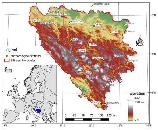
Figure 1.
Geographic location of BiH with altitudes and location of weather stations considered in the study (http://www.ikc-berlin.de/bosnisch/html/bosna/KARTE-BOSNE.htm (accessed on 5 February 2023) and http://www.bosnaonline.org/opce-karte-bosne-i-hercegovine (accessed on 5 February 2023)).
The analyzed territory in this study spans between 42°30′ and 45°20′ latitude and between 15°40′ and 19°40′ longitude. The weather data were gathered from 18 meteorological stations throughout BiH, with the addition of one border station in the Republic of Serbia (RS) and one in the Republic of Croatia (RC). The purpose of including these border stations is twofold. First, their data is used for data interpolation, which helps to fill in the gaps and provide more comprehensive coverage of climatic conditions in the eastern and northern parts of BiH. These areas are relatively poorly covered by the existing meteorological stations within BiH. Second, by considering the climatic conditions in these neighboring regions, the study aims to capture a more accurate representation of the overall climatic patterns within the analyzed territory.
Figure 2 presents the land cover for Bosnia and Herzegovina, with its five main and dominant types.
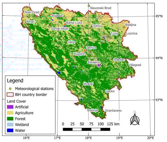
Figure 2.
Land cover in BiH. (https://land.copernicus.eu/faq/about-data-access (accessed on 5 February 2023)).
The dominant land cover in BiH is forested land (Figure 2), which covers more than half (54.6%) of the country’s territory [35]. These forests primarily consist of broad-leaved forests. The northern and northeastern parts of the country are mainly characterized by agricultural land, where arable land and crops are present [36]. Agricultural land, including pastures and meadows, accounts for 42.2% of the total land cover [35]. Arable land accounts for 19.6% of the total agricultural land. Artificial areas, such as urban and built-up areas, account for 2% of the land cover. Wetlands and water bodies make up a smaller portion, with wetlands occupying 0.1% and water bodies covering 1% of the total land area. The remaining land cover percentages are attributed to less dominant categories such as semi-natural vegetation and open spaces/bare soils [37].
The meteorological stations are distributed almost regularly throughout the country and cover all the altitudes at which agricultural production is carried out. They are shown in Table 1.

Table 1.
Name, altitude (ALT), latitude (LAT), and longitude (LONG) of the meteorological stations used in the analysis.
In the study, the altitude of meteorological stations in BiH was in a range of 97 m above sea level (m.a.s.l.) in Bijeljina to 947 m.a.s.l. in Gacko. Although the Slavonski Brod meteorological station had the lowest altitude (88 m.a.s.l.), this is not considered relevant since it belongs to Croatia. As mentioned before, the inclusion of the Slavonski Brod station serves the purpose of capturing climatic conditions in the neighboring region rather than for altitude-related analysis within BiH.
The daily measurements of the weather parameters for the common irrigation season were available at the studied meteorological stations and were used to calculate ETo. Using the daily input data, the average values of daily, monthly, and annual basic weather parameters during the common irrigation season (April–October) were calculated. In Table 2, an overview of these average values for the periods of 2000–2005 and 2018–2022 is presented. The global aridity index [38] was used to classify meteorological stations into different zones, and it is presented also in Table 2. The aridity index is a metric defined by the United Nations Convention for Combat Desertification, and it represents the ratio of mean annual precipitation to mean annual ETo calculated in this study [38]. Aridity indices [39,40] provide a measure of available moisture to the specific crop potential growth [39]. In this research, precipitation data were collected from the meteorological stations at the respective hydrometeorological institutions, and ETo data were calculated using the FAO-PM method [1]. In the first observation period, meteorological stations were categorized into two zones, dry sub-humid (DSH) and moist sub-humid (MSH). In the second observation period, in addition to DSH and MSH zones, a semi-arid (SA) zone emerged.
Table 2.
Input data set, climatic zones with respect to the P/ETo ratio, analyzed periods, and source of the data.
In Table 2, the following weather data are presented: P—precipitation (mm), average sum for irrigation season; Tmax—maximum air temperature (°C); Tmin—minimum air temperature (°C); Tavg—mean air temperature (°C); RHmax—maximum relative humidity (%); RHmin—minimum relative humidity (%); RHm—mean relative humidity (%); n—duration of sunshine hours (h), average sum for irrigation season; Rs—solar radiation (MJ m−2 day−1); u—average wind speed (m s−1) measured at 10 m height; ETo—reference evapotranspiration estimated by the FAO-PM approach (mm), average sum for irrigation season.
The meteorological stations in the study were equipped with mercury and alcohol thermometers for measuring the temperature, a rain gauge for precipitation measurement (mm), a Campbell–Stocks heliograph for the measurement of sunshine duration (h), as well as an anemometer set at 10 m height for capturing the wind speed in m s−1. Air relative humidity was determined using a psychrometer calculator, which is based on readings of a dry bulb thermometer and a wet bulb thermometer, partial vapor pressure, and dew point temperature. The sensors are maintained regularly according to the standards of the World Meteorological Organization (WMO).
The daily weather data were collected and elaborated for the common irrigation season, which spans from April to October, for two different time periods, 2000–2005 and 2018–2022. These two periods were selected based on the availability of good-quality data for all locations. However, for the second study period (2018–2022), two stations (Jajce and Grančarevo) were excluded from the analysis, since there were no accessible weather data. Regarding stations from the Republic of Serbia and Croatia (Loznica and Slavonski Brod), the period of analysis (2018–2022) is missing the last two years (2021 and 2022), since we could not obtain data for those years. Furthermore, the months from November to March were not taken into consideration due to frequent occurrences of precipitation and snowfall during these months, which poses challenges in the maintenance of weather stations and the collection of accurate data.
The analysis of the aridity index (P/ETo ratio) for the 2000–2005 and 2018–2022 periods in BiH reveals some significant findings. In both periods, the majority of BiH falls into the MSH zone, with 13 out of 18 stations in the first period and 10 out of 16 stations in the second period falling into this category. However, a notable change occurs between the two periods. In the second period, there is a substantial decline in precipitation and an increase in evapotranspiration observed across all stations in BiH. This reduction in precipitation leads to the emergence of a new climate zone, the semi-arid zone (SA), which was not present during the first period. The station in Gacko experienced the most significant reduction in precipitation, with a decrease of 184 mm. This reduction classifies Gacko as having a DSH climate character. Similarly, although Bijeljina showed a slight decrease in evapotranspiration, the reduction in precipitation by 162 mm places this station in the semi-arid climate type. The decreasing trend of the aridity index in the second period indicates potential significant climate changes in the next decade or so within the territory of BiH. These changes suggest a shift towards drier conditions and increasing aridity, which can have substantial impacts on the environment, agriculture, and water resources in the region.
The areas located in the DSH zone primarily encompass the eastern, southeastern, and southern parts of BiH. In this zone, the ETo values during the common irrigation season (April–October) were higher than 750 mm. On the other hand, the MSH zone includes the western, northwestern, and northeastern parts of BiH, where the ETo values for the common irrigation period were lower than 750 mm.
The aridity index for the 2018–2022 period in BiH indicated that 4 stations out of 16 (25%) entered the SA zone (Bijeljina, Višegrad, Trebinje, and Mostar), whereas 2 stations remained in the DSH zone (Banja Luka and Gacko). A noteworthy change occurred at the Banja Luka station, which transitioned from the MSH zone to the DSH zone during the second period analyzed. This suggests an increase in aridity and drier climate conditions in that area. Regions that were previously characterized by abundant precipitation and favorable conditions for rainfed agriculture are now experiencing a shift towards dry semi-arid climate conditions.
2.2. Data Quality Analysis, Elaboration, and Adjustment
2.2.1. Data Quality Analysis
A quality assurance and correction process was conducted on the collected daily weather data following the procedure proposed by Allen et al. [1,41]. This process involved implementing control measures to ensure the accuracy and reliability of the data. Table 3 shows the percentage of input daily data failures that were corrected using the procedure described below.
Table 3.
Input daily data error for common irrigation season during two periods of observation.
To identify errors in the meteorological parameters, lower and upper thresholds were set. Any data falling outside of these thresholds were flagged as potential errors. Most of the errors encountered were attributed to poor data entry during the manual input into the electronic database. To minimize such errors, data entries without logical inconsistencies were discarded. In the case in which the error was logical and recognizable, such as a comma, or maximum and minimum temperature values were swapped, the data were compared with the original record in the meteorological log and then corrected. These errors mostly occurred in the data of the first observation period and with the stations in Bijeljina, Banja Luka, and Trebinje (Table 3).
For parameters that exhibited illogical errors, adjustments and corrections were made by referring to the average values of those parameters at the corresponding time from neighboring stations with similar climatic characteristics. This approach allowed for the estimation and rectification of erroneous values based on the surrounding data.
2.2.2. Missing Data
During the analysis of the meteorological data, it was observed that some weather parameters were missing for certain individual records and days at some of the meteorological stations for both observation periods. Specifically, the missing data pertained to relative humidity (RH), sunshine duration (n), and windspeed (u), as indicated in Table 3. In the second observation period, seven meteorological stations lacked data on maximum (RHmax) and minimum (RHmin) relative humidity for the years 2021 and 2022. In addition, the Gacko, Loznica, and Slavonski Brod stations had extended periods or even entire seasons with missing data. An additional discrepancy arose during the first observation period, for which data on the sunshine duration were conspicuously missing at six stations. However, it is worth noting that during the subsequent observation period, a comprehensive record of sunshine duration data was accessible for almost all stations, which meant a significant improvement in data collections and recording practices. Windspeed data were notably missing, with up to 20% of data being absent for the Zenica station (Table 3). To address these issues, a procedure was followed to estimate missing data based on available information.
If wind data were not available for a particular station, data from a neighboring station were utilized if they existed for the same period and if the neighboring station had similar climatic and orographic characteristics. This approach allowed for the use of reliable wind data from a nearby location to fill in the gaps at the station with missing data. In cases in which there was no similarity with the neighboring station, the mean value of the same parameter was used for the corresponding period from the remaining examined years in which the measurements existed. The same procedure was applied to the daily values of maximum and minimum air temperature, as well as the sunshine duration.
In the absence of directly measured daily relative humidity, the missing data were calculated using the formulas proposed by FAO 56, which provide a method for estimating relative humidity [1]. The estimation of the actual vapor pressure (ea) was performed based on the dew point temperature (Tdew), which was assumed to be equal to the daily minimum temperature (Tmin). This assumption is valid for humid regions where, at sunrise, the air temperature is close to Tmin. In that case, the air is nearly saturated with water vapor, resulting in almost 100% relative humidity. If we assume that Tmin represents Tdew, then we can use Equation (1) to calculate ea as:
Relative humidity was calculated as:
where e°(Tmin) is the actual vapor pressure at the minimum temperature, and e°(Tmax) is the actual vapor pressure at the maximum temperature [kPa].
At some stations (Table 3), there were only mean values of relative humidity (RHm). At these stations, the actual vapor pressure (ea) was calculated using the expression:
where es is saturation vapor pressure [kPa], and ea is actual water pressure [kPa].
The solar radiation (Rs) data were not available at all stations in the first period of observation (Table 3); thus, the value of Rs was estimated using the method recommended by FAO 56 [1]. There are two formulas used for Rs estimation, depending on whether data on the duration of sunshine (n) in hours were available. For the stations for which n was not measured, the Hargreaves radiation formula was applied:
where Ra is extra-terrestrial radiation (MJ m−2 day−1), and KRs is the empirical correction coefficient, which is 0.16 for inland areas and 0.19 for locations in the coastal area.
At other stations, n was measured, and Rs was calculated using the Angstrom expression:
where n is the actual sunshine duration (h), N is the maximum sunshine duration (h), as = 0.25, and bs = 0.5.
2.2.3. Solar Radiation Data Analysis and Correction
The accuracy of solar radiation (Rs) data was assessed by comparing them to solar radiation on a clear day, known as Rso (reference solar radiation). The ratio of Rs to Rso was plotted graphically in relation to the day of the year for each examined station. In this study, Rso was calculated using the method proposed by Allen [41] as:
where Rso is clear-sky solar radiation (MJ m−2 day−1), and z is station elevation above sea level (m).
Since Rso is the maximum solar radiation that reaches the Earth’s surface on any given day, the curve Rs/Rso shows the errors that might have occurred for determining Rs. In cases in which the measured Rs values were below the Rso curve, a correction was performed to adjust the Rs values. The Rs correction was performed at all tested meteorological stations, involving the determination of correction coefficients through trial-and-error methods for each year separately. The correction coefficients were derived to bring the measured Rs values closer to the expected values based on the Rs/Rso curve. The specific values of the correction coefficients for each year are presented in Table 4 in the Results and Discussion section of this study. The corrected values of Rs were used for further analyses.
Table 4.
Correction coefficients for Rs at the studied meteorological stations (2000–2005 and 2018–2022).
2.3. Methods Used to Estimate Reference Evapotranspiration (ETo)
In the study, the reference evapotranspiration (ETo) was calculated on a daily basis for each meteorological station, considering both study periods: 2000–2005 and 2018–2022. Nine empirical methods were compared with ETo estimated using the FAO-PM method [1]. The selection of the empirical methods was based on previous studies and their application in the region.
2.3.1. FAO Penman–Monteith Method (FAO-PM)
The FAO Penman–Monteith approach (FAO-PM) is considered to be a standard method for ETo estimation. According to Allen et al. [1], it is expressed as:
where ETo is reference evapotranspiration (mm day−1), Rn is net radiation at the crop surface (MJ m−2 day−1), G is the soil heat flux density (MJ m−2 day−1), γ is a psychrometric constant (kPa °C−1), T is the mean daily air temperature at 2 m height (°C), U2 is the average windspeed measure at 2 m height (m·s−1), es is saturation vapor pressure (kPa), ea is actual vapor pressure (kPa), es − ea is the saturation vapor pressure deficit (kPa), and Δ is the slope vapor pressure curve (kPa °C−1). The mentioned parameters are calculated using standard procedures proposed by FAO 56 [1].
2.3.2. Hargreaves–Samani Method (HS)
The Hargreaves–Samani method (HS) is based only on maximum and minimum air temperatures, and it is expressed as:
2.3.3. Modified Hargreaves–Samani Method
The modified Hargreaves–Samani (HM) method [42,43] is derived by the calibration of the exponent 0.5, which is changed to 0.424. Calibration of the exponent 0.5 was performed according to regional analysis of data from three locations (Niš, Palić, and Sarajevo). The HM method is expressed as follows:
2.3.4. Calibrated Hargreaves–Samani Method (HC)
In this method, the Hargreaves exponent, which is set to 0.5, was modified for all the meteorological stations during the common irrigation season. Calibration of the exponent 0.5 was performed by comparing the HS method with the FAO-PM method, with the new exponent being accepted when the regression coefficient (b) had a value of one. This iterative process was replicated for each meteorological station and for each common irrigation season. The HS method calibrated in this manner, with the adjusted exponent value, is referred to as the calibrated Hargreaves–Samani method (HC). The calibration of the Hargreaves exponent aimed to improve the accuracy and agreement of the HS method with the FAO-PM method in estimating reference evapotranspiration.
2.3.5. Priestley–Taylor Method (PT)
The Priestley–Taylor method is a simplified Penman method expressed as follows:
where α = 1.26, Δ is the slope of the saturating vapor pressure versus temperature (mb °C−1), γ is the psychometric constant (kPa °C−1), and λ is the latent heat of vaporization (λ = 2.45 MJ kg−1 at 20 °C).
2.3.6. Makkink Method (MAK)
The Makkink method is also known as the radiation method. It was published in 1957 [44], and it is expressed as:
2.3.7. Copais Method (COP)
The Copais method is derived using bilinear polynomial regression analyzing meteorological data specific for the central Greece region [45]. This method was chosen based on its demonstrated good performance in moderate climate conditions. The formula is expressed as follows:
where ETo is reference evapotranspiration (mm day−1), m1 = 0.057, m2 = 0.277, m3 = 0.643, and m4 = 0.0124.
C1 and C2 can be calculated according to the formulas:
where RH—mean air relative humidity (%), T—average air temperature (°C).
2.3.8. Penman–Monteith Method with Limited Data Availability—Based on Air Temperature Data (PMT)
The temperature-based Penman–Monteith method used in this research requires the minimum and maximum air temperature to estimate the reference evapotranspiration (ETo). However, for windspeed, a global average value of 2 m/s (U2g) is proposed as a default when site-specific data are unavailable [1]. Previous studies have indicated that using a regional (U2r) or local (U2l) value for windspeed yields better results compared to the global value of U2g = 2 m s−1 [46,47]. In the countries of the former Yugoslavia, it has been determined that the regional value for windspeed is U2r = 1.3 m·s−1. The local value of windspeed (U2l) was obtained as a local average from meteorological observations over a period of 30 years (1961–1990). Since the windspeed measurements at the examined meteorological stations were taken at a height of 10 m, correction was needed to estimate the windspeed at a height of 2 m. Correction was performed using the following formula:
where U10 is the windspeed measured at 10 m height (m s−1).
Penman–Monteith Method Based on Air Temperature and Overall Average Windspeed (PMT2)
To calculate ETo with this method, only data for the maximum and minimum air temperature are required, and 2 m s−1 is adopted for windspeed.
where U2g is the global windspeed (2 m s−1).
Penman–Monteith Method Based on Air Temperature and Regional Average Windspeed (PMT1.3)
For this version of the PMT method, only the data for the maximum and minimum air temperature are required, and for the windspeed, the regional value of 1.3 m s−1 is adopted in the countries of the former Yugoslavia.
where U2r is the regional wind speed (1.3 m s−1).
Penman–Monteith Method Based on Air Temperature and Site-Specific Windspeed (PMTlok)
Using this version of the PMT method, the site-specific average wind speed was calculated for each station for the period from 1961 to 1990.
where U2l is the local wind speed (m s−1).
In this paper, the three PMT methods are tested to assess improvements in the estimation of reference evapotranspiration (ETo) by incorporating more accurate windspeed data.
2.4. Statistical Evaluation of the Methods’ Performance
In this study, various statistical indicators were used to compare the estimates of reference evapotranspiration (ETo) obtained from empirical methods with those obtained from the standard FAO-PM method. These statistical indicators were chosen based on their wide applicability in hydrological studies and their ability to provide insights into the accuracy and performance of the different methods [24,25,31,38,46].
A comparison of measured and estimated values of daily ETo was performed using a simple linear regression, in which the measured values of ETo were taken as a dependent variable b (slope), the estimated values of ETo were taken as an independent variable x, n is the number of tested values, Pi is estimated value, and Oi is measured value. The slope of linear regression was estimated as:
The determination coefficient (R2) is a statistical indicator that assesses the representativeness of a regression model, which is based on the analysis of variance. It is calculated as the ratio of the sum of squares of the deviations interpreted by the regression model to the total sum of squares of the deviation. In other words, it represents the percentage of the total variation in the dependent variable (y) that is accounted for by the regression model.
The root mean square error (RMSE) is a statistical indicator that measures the variability or dispersion of the residuals between the predicted values (Pi) and observed values (Oi) in the same units as Oi. It provides a measure of the average magnitude of these residuals and serves as an estimate of the standard deviation of the errors. A smaller RMSE indicates a better model performance. The RMSE is given as:
Since the RMSE is expressed in variable units, it is much more convenient and easier to interpret than the R2.
The mean absolute error (MAE) quantifies the average magnitude of the simulation error. The MAE provides a measure of the average absolute deviation between the predicted and observed values regardless of the direction of the errors.
The mean relative error (MRE) represents the mean relative error in % that shows the magnitude of the error in relative terms. It indicates the percentage of the observed value by which the predicted value deviates on average.
The maximum absolute error (Emax) represents the maximum deviation or difference between a predicted value (Pi) and its corresponding observed value (Oi) in a data set.
The Nash–Sutcliffe efficiency coefficient (NSE) is a dimensionless indicator that represents the ratio of the mean square error and the variance of the measured values. The NSE provides a measure of the performance of the model in relation to the observed values. The best method is one in which the NSE value is close to one, and at the same time, the RMSE parameter shows the lowest value.
The index of agreement (dlA) is a descriptive indicator that measures the agreement or similarity between observed and predicted values. It is an indicator of the degree to which the prediction model is free of error. The index of agreement is a dimensionless indicator whose value ranges from 0 to 1, where a value of 1 indicates an ideal fit. It represents the ratio between the mean square of the error and the “potential error” defined as the sum of the squares of the absolute value of the distance from ETo, pm and ETo, eq to eq and represents the highest value that can be achieved for each pair of measured and estimated models.
2.4.1. TOPSIS Ranking Method
The ideal point method, TOPSIS [32], is well known as a multicriteria method used to rank a given number of alternatives assessed across selected evaluation criteria. In this case study, alternatives are methods for estimating reference evapotranspiration, and criteria are the root mean square error (RMSE), mean absolute error (MAE), mean relative error (MRE), maximum absolute error (MAE), the Nash–Sutcliffe efficiency coefficient (NSE), and the index of agreement (dIA). Before the 6 steps of the TOPSIS procedure start, a performance matrix needs to be created. The performance matrix is used to quantify the performance of each method for each criterion and is presented as follows:
where alternatives A1, A2, …, An represent the set of methods for estimating reference evapotranspiration, and rij (i = 1, … n, j = 1, …, m) is the evaluation criterion, i.e., the value of the jth error of the ith alternative across m criteria. In general, the weights of criteria w1, w2,…, wm above the matrix can be defined by experts or by other means—here, it is assumed that all weights are equal (all criteria have the same importance for the evaluation of alternatives). The TOPSIS method evaluates alternatives in 6 steps:
- 1.
- Constructing the normalized decision matrix to convert various attribute dimensions to nondimensional ones. Elements of the normalized decision matrix are calculated as follows:
- 2.
- Constructing a weighted normalized decision matrix. A weighted normalized decision matrix is obtained by multiplying the values in the columns of the normalized matrix by the corresponding criterion’s weight.
- 3.
- The identification of the best (“ideal solution”, A*) and the worst (“negative—ideal solution”, A−) values in each column.
- 4.
- Computing the separation measure.
The Euclidian distance is used to measure the separation of each alternative from the ideal (Si*) and negative ideal solution (Si−).
- 5.
- Calculating relative closeness to ideal solution.
This step is calculated by the following equation:
where Si* is the distance of the ith alternative from the ideal positive solution; Si− is the distance from the ideal negative solution; and Si+ is the distance from the ideal positive solution.
- 6.
- Ranking alternatives. The best-ranked alternative has the value of Qi* closest to 1.
2.4.2. Mann–Kendall Test (MK)
This is a rank-based nonparametric statistical test that was developed by Mann in 1945 and Kendall in 1975 [34]. It is commonly used to detect trends, both linear and non-linear, in time series data. The Mann–Kendall test assesses the null hypothesis (Ho) that there is no trend in the data, whereas the alternative hypothesis (H1) assumes the presence of a trend [48]. The Mann–Kendall test statistic, S, measures the number of concordant pairs (where the ranks have the same order as the original data) minus the number of discordant pairs (where the ranks have the opposite order as the original data). A positive value of S indicates an increasing trend, and a negative value indicates a decreasing trend. The magnitude of S represents the strength or magnitude of the trend. The Mann–Kendall test statistic S is computed as follows:
where xi and xj are the sequential data values of the time series in the years i and j; i = 1, 2, 3, …, n − 1 and j = i + 1, i + 2, i + 3, …, n; n is the length of the time series.
The variance (σ2) for the S-statistic is defined by:
The standard test statistic Zs is calculated as follows:
If |Zs| is greater than Zα/2, where α denotes the chosen significance level (5% with Z0.025 =1.96), the null hypothesis is invalid, implying that the trend is significant [48].
In the research conducted, the Mann–Kendall (MK) test was performed to analyze monthly and seasonal trends for the 2018–2022 period at three representative stations located in different climate zones. The selected stations were Trebinje (representing a SA zone), Gacko (representing a DSH zone), and Sanski Most (representing a MSH zone). Stations were chosen based on the best-ranked method within their respective climate zones. To conduct the MK test and calculate the trend, the researchers utilized the MAKESENS Excel template [49]. MAKESENS is an Excel tool that was developed during a research project between Nordic and Baltic countries, as part of the EMEP (Evaluation of the Long-Range Transmission of Air Pollutants in Europe) 20-year assessment. This template provides a user-friendly interface for performing the Mann–Kendall test and analyzing trends in environmental data. During the analysis, the MAKESENS procedure calculated the confidence interval for the trend at two different confidence levels: α = 0.01 and α = 0.05. These confidence intervals provide information about the range of values within which the true trend parameter is likely to fall. The use of two different confidence levels allows for the assessment of the uncertainty associated with the estimated trend.
2.4.3. Sen’s Slope Evaluation
Sen’s slope, also known as the Sen’s estimator or the Mann–Kendall estimator, is a robust non-parametric method recommended by the WMO for trend detection in hydrological studies [50]. It is widely used to quantify linear trends and assess changes over time in various environmental and hydrological variables. One advantage of Sen’s slope is its robustness to outliers or data errors, unlike traditional linear regression methods [51]. It is a resistant estimator that provides a reliable measure of the trend even in the presence of extreme values or data inconsistencies.
The equation for Sen’s slope, which is used to calculate the trend, can be written as follows:
where xj and xi are data values at time j and i (j > 1), respectively. If there are n values of xj in the time series, there will be N = n(n − 1)/2 slope estimates [51]. The N value of Qi is sorted from smallest to largest, then Sen’s slope uses median Qi (Qmed). A two-tailed test estimated the value of Qmed at a confidence interval of 90% and 95%, which is calculated as:
A 100(1 − α) % two-sided confidence interval about the slope estimate is obtained by the nonparametric technique based on the normal distribution. The method is valid for n as small as 10, unless there are many ties.
In this research, the magnitude of the Sen’s slope trend was derived using the MAKESENS Excel tool.
3. Results
3.1. Correction of Solar Radiation Data
Solar radiation (Rs) is shown to be an important parameter for ETo calculation [52,53,54]. In this study, the accuracy of the Rs estimate was checked through the Rs and Rso ratio curve. The corrected values of Rs were used for further analyses, and the correction coefficients were estimated for all studied years at the examined meteorological stations, as shown in Table 4. The correction coefficient varies from site to site and from one year to another. The highest correction was necessary for almost all the years for the station of Trebinje, located in the southeastern region of the country and characterized with low precipitation particularly during the summer season. This indicates the possibility of a systematic error in the Rs estimate at that location, potentially due to inadequate maintenance of the equipment. Additionally, significant correction was also needed for the stations in Tuzla and Zenica, in the central region of BiH. Both locations are very well known and are important industrial zones for carbon excavation and the production of electric energy. Therefore, the air pollution from these industrial activities likely contributed to the underestimation of Rs values. However, at some other locations, the corrections were minimal. In the first observed period (2000–2005) at the Višegrad meteorological station, the correction of Rs was not made due to ability of Rs to reach Rso curve. Comparatively, at the Mostar meteorological station, the same coefficient was used in all studied years (1.06) during the 2000–2005 period. In the second period (2018–2022), the meteorological stations at Grančarevo and Jajce were not taken into consideration due to a lack of input data. The same is true for the Loznica and Slavonski Brod stations, both from bordering states, since there were no available data from 2021 and 2022.
3.2. Calibrated Hargreaves–Samani Method (HC)
The calibration of the HS method has been performed for many locations worldwide [42,43,55]. In this study, the calibration of the HS method was performed for each station and for both analyzed periods, as explained in Section 2.3.4. The new coefficient (exponent of the third term) in Equation (8), which represents the differences between the maximum and minimum air temperature, was obtained using a trial-and-error method. An example of the calibration process for the Bijeljina meteorological station is shown in Figure 3.
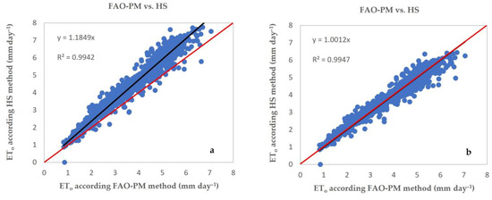
Figure 3.
Linear regression between the reference evapotranspiration estimated by the HS equation and by the FAO-PM method for location of Bijeljina (2000–2005) before (a) and after calibration (b) of HS equation.
The calibrated exponents for the period 2000–2005 are presented in Figure 4. To obtain calibrated exponents for the entire country, spatial interpolation techniques were used, including the Topo grid (“Spline” interpolation) and RST (“Regulated Spline with Tension”). The spatial interpolation methods aim to predict values across the entire study area based on the available data and to reduce the curvature of the resulting surface. These methods have been widely used in hydrological and climatological studies to predict variables and achieve a smooth representation of the spatial distribution. In this study, ArcGIS 10.1 was used for the map production of calibrated coefficients.
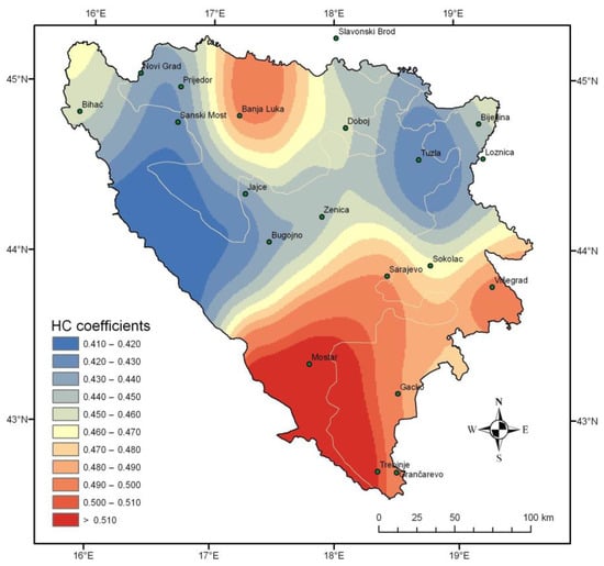
Figure 4.
Spatial variation of the calibrated coefficients for HC method.
During both observation periods, calibrated exponents in the HS equations varied across different regions in BiH. The calibration of the exponent is mainly influenced by topographic characteristics, weather data (such as air temperature and windspeed), and the proximity to large bodies of water. The western and northeastern parts of BiH had the lowest calibrated exponents, ranging from 0.410 to 0.460. On the other hand, the northern, eastern, and southeastern parts had the highest values, ranging from 0.460 to 0.500.
Furthermore, a linear relationship was established between the calibrated exponent of the HS equation and the ratio of precipitation to reference evapotranspiration (P/ETo). The calibrated exponent in the HS equation becomes larger when the ratio of precipitation to reference evapotranspiration (P/ETo) is 0.5 or lower. The higher value of the calibrated exponent in the DSH zone suggests that in that part of BiH, there is higher humidity and windspeed compared to the MSH zone. The HS method, however, does not explicitly consider humidity and windspeed, leading to the need for calibration.
Many authors have proposed calibration of the HS method exponent to improve its performance in different climate conditions and regions of the world [55,56,57]. This is also reported by Trajkovic [58], who performed regional calibration of the HS method on seven meteorological stations in Serbia. Although calibrated, the ETo values were about 13% higher than those obtained by the FAO-PM method. The exponents obtained by the calibration of the HS method in the territory of BiH for the crop growing period in 2000–2005 ranged from 0.411–0.525, and for the period of 2018–2022, the coefficients were in the range of 0.413–0.535. Similar results were obtained by Trajkovic and Zivkovic [59], indicating consistency in the findings. In terms of the performance of the HS method in different climate zones, it was found to have an average overestimation of about 4% in the DSH zone and 3% in the SA zone during both the 2000–2005 and 2018–2022 periods. These results are consistent with other studies [38,60], which have also reported slight overestimation by the HS method in certain climate zones.
3.3. The Performance of Empirical Methods for ETo Estimation
Statistical analysis was performed in order to evaluate the empirical methods for ETo estimation and their performance in a different climate zone in BiH. The statistical parameters were averaged and are presented by climatic zones as an average for both analyzed periods (2000–2005; 2018–2020) in Table 5 and Table 6.
Table 5.
Average statistical parameters of the different ETo calculation methods’ performance for common irrigation period (2000–2005) and their rank in the BiH climatic zones.
Table 6.
Average statistical parameters of the different ETo calculation methods’ performance for common irrigation period (2018–2022) and their rank in the BiH climatic zones.
According to Table 5, which presents average statistical parameters for the DSH and MSH zones during the 2000–2005 period, two methods stood out as the best-ranked in both zones according to the TOPSIS ranking method. In the DSH zone, the HC method was ranked as the best method, whereas in the MSH zone, the PT method took the first place. The difference in rankings can be attributed to variations in climate-dependent factors between the two zones. In the DSH zone, the PMT2 and HS methods also ranked well, providing a 4% underestimation and overestimation of ETo, respectively. On the other hand, the COP method obtained the lowest-ranking position in the DSH zone. In the MSH zone, the PT method achieved the highest rank, followed by the HM and HC methods. Conversely, the HS method obtained the lowest rank in the MSH zone.
These rankings indicate that the performance of different methods highly depends on the specific climatic conditions and factors within each zone. The HC method performed well in the DSH zone, whereas the PT method was more suitable for the MSH zone during the first period of observation. In Appendix A, Appendix B, Appendix C, the ranks of the methods for all analyzed stations in both zones during the 2000–2005 period are presented, calculated using the TOPSIS method.
In Table 6, the average statistical parameters for the 2018–2022 period are presented. From this table, it can be seen that in the second period of observation, significant changes occurred in comparison to the first period. These changes can be attributed to climate changes and more frequent extreme weather events that gradually evolved over time. Some of the meteorological stations in the DSH zone experienced reduced precipitation and increased evapotranspiration, leading to drier conditions. As a result, these stations shifted from the DSH zone to the semi-arid (SA) zone.
In terms of statistical methods used, the HC method was ranked as the best method across all three zones (SA, DSH, and MSH). However, in the SA zone, alternative methods such as the PMTlok and COP method showed promising results as well. In the DSH zone, the PMT1.3 and PMTlok methods could be considered as alternatives. In the MSH zone, in addition to the HC method, the MAK and PT methods also ranked well. On the other hand, in the DSH zone, the MAK and COP methods obtained the two lowest-ranking positions out of the nine tested methods. Similarly, in the MSH zone, for the second period, the lowest-ranked method was the HS method, as was the case in the first period of observation. In the SA zone, the lowest-ranked was the HM method. As an overall result of statistical analysis for the 2018–2022 period, it can be concluded that the HC method consistently performed well across the different zones, but alternative methods showed potential in specific zones and stations. Appendix D, Appendix E, Appendix F, Appendix G contain the ranks of the methods for all analyzed stations in both zones during the period from 2018 to 2022. These ranks have been calculated using the TOPSIS method, which is a multi-criteria decision-making technique used to evaluate and rank alternatives based on their performance across multiple criteria.
In Figure 5, the spatial distribution of the daily values of ETo calculated by the FAO-PM method (2018–2022) is presented.
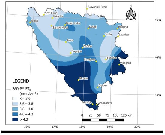
Figure 5.
Values of ETo (mm day−1) calculated using the FAO-PM method (2018–2022).
Figure 5 reveals a distinct spatial pattern in reference evapotranspiration (ETo) values across Bosnia and Herzegovina. The highest ETo values are prominently observed in the southern and southeastern regions of the country. These areas are characterized by traits of a dry sub-humid and semi-arid climate. In contrast, the lowest ETo value is recorded in the northeastern sector, encompassing Novi Grad and Prijedor, where a moist sub-humid climate prevails.
To further elucidate, Figure 6 illustrates the disparity between the HC method, which emerged as the top-ranking technique during the second observation period (2018–2022), and the FAO-PM method.
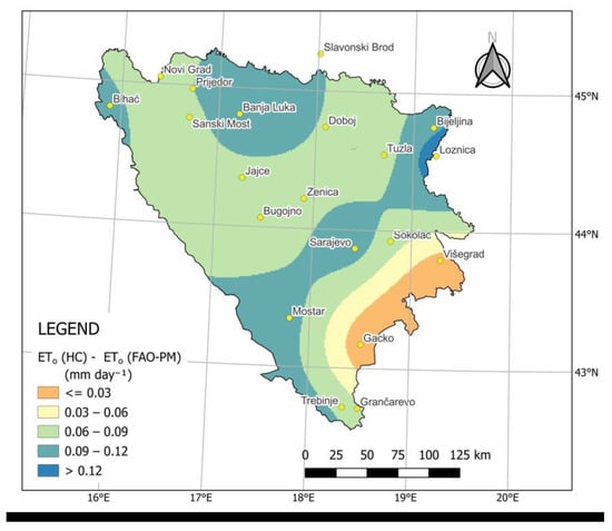
Figure 6.
Difference between HC and FAO-PM methods (2018–2022).
The HC method demonstrated the highest degree of agreement with the FAO-PM method, particularly evident at meteorological stations situated in the southeastern part of BiH. Notably, at stations such as Gacko and Višegrad, the deviation in the HC method from the FAO-PM method was notably minimal and amounts to less than 0.03 mm day−1. These stations are characterized by prevailing semi-arid climatic conditions.
Conversely, the most significant differences compared to the FAO-PM method were observed at stations characterized by distinct moist sub-humid and dry sub-humid climate traits. At these specific stations, the deviations ranged between 0.09 and 0.12 mm day−1, highlighting the relatively greater divergence in ETo estimations.
3.4. Mann–Kendall Test Performance
Trends in the time series of values of evapotranspiration were detected and estimated using the nonparametric Mann–Kendall test. In this study, time series consisted of fewer than 10 data points; hence, the S test is used. The magnitude of the trend is estimated by the nonparametric Sen’s slope method. The Mann–Kendall test is performed on three stations, each of them representative of the specific zone, and for the 2018–2022 period. Evaluation is performed on a monthly and seasonal basis.
Results of the calculation of the S test using the averaged data for the April–September period show that there is an upward trend for the Trebinje station (S = 8), shown in Figure 7, with a 0.1 level of significance (α = 0.1; there is a 10% probability that a mistake is made when rejecting null hypothesis of no trend).
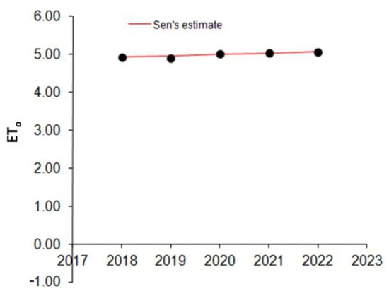
Figure 7.
Upward trend of reference evapotranspiration for the Trebinje station using MAKESENS 1.0 [49].
For the Gacko (DSH zone) and Sanski Most (MSH zone) stations, there is also a potential that the trend is upward (S = 6), but the level of significance is low (α greater than 0.1).
In Table 7, the monthly trends detected for given periods for all three stations are summarized.
Table 7.
Monthly trends and significance for Trebinje, Gacko, and Sanski Most stations.
For all three stations, the trend of increasing evapotranspiration in the month of July is significant. For the Trebinje station, a significant trend is also detected for August, but with a downward trend. This is in accordance with findings in Canada and India [61,62]. In Figure 8, the month with a significant trend for three stations is presented.
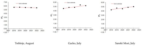
Figure 8.
The months with significant trends for each of the representative stations.
Figure 8 illustrates the trends observed for three different stations: Gacko, Sanski Most, and Trebinje. The figure indicates that significant trends were observed in July for Gacko and Sanski Most, and for Trebinje, a significant trend was observed in August. For both Gacko and Sanski Most, the trend was upward (S = 8). Additionally, the significance level associated with these trends was high, indicated by a value α = 0.1. On the contrary, for Trebinje, a downward trend was recorded, indicated by S = 8. This implies that there was a negative trend in the data for this station in August. Similarly, the significance level associated with this trend was high (equal to 0.1).
4. Discussion
In the DSH zone of BiH, the average root mean square error (RMSE) of the HS method during the common irrigation season (2000–2005) was 0.77 mm day−1. In the MSH zone, the average RMSE of the HS method was higher, at 0.98 mm day−1. The largest deviation, reaching up to 27%, was observed during the common irrigation season. These findings are consistent with similar studies conducted in other regions [45,63].
In the MSH zone, the HS method exhibited the highest average overestimate of 18% for both periods of observation. Additionally, the RMSE of the HS method (0.98 mm day−1) was 43% higher compared to the RMSE of the HC method (0.56 mm day−1) during the 2000–2005 period. The disparity between the HS and HC methods persisted in the period from 2018 to 2022, with the HS method showing a 47% higher RMSE value in the MSH zone compared to the HC method. Among the nine meteorological stations analyzed, the overestimation of the HS method exceeded 20% in all cases. The highest overestimate was observed at the Tuzla meteorological station, reaching +27% during the 2000–2005 period. This significant deviation indicates that the HS method is not suitable for accurate estimation of reference evapotranspiration (ETo) in the MSH zone. These results align with findings from other studies that have tested the HS method in humid regions around the world [64,65,66]. The study conducted by Trajkovic and Kolakovic [64] in the humid condition of Croatia (southeast Europe) at the Belje station reported an even greater overestimation of 41% using the HS method. In comparison, an average root mean square difference (RMSD or RMSE) value of 0.9 mm day−1 was obtained at 48 sites in 16 states in the USA [67]. Interestingly, the average RMSE for the common irrigation season in the two examined zones in BiH (2000–2005) was also 0.9 mm day−1, which is identical to the value obtained in the United States. However, in the subsequent period (2018–2022), the average RMSE for the three zones in BiH decreased to 0.83 mm day−1. Another assessment of the HS method was carried out on a daily basis in the Andalusia region of southern Spain [68]. The results indicated deviations of the HS method from the FAO-PM method, with average lower values of ETo (0.69 mm day−1) observed at coastal stations and higher values of ETo (0.13 mm day−1 higher) compared to the ETo obtained by the FAO-PM method at inland stations. In the examined areas of BiH, specifically in the moist sub-humid (MSH) zone, the average ETo obtained by the HS method during the common irrigation season was 0.73 mm day−1 higher than the ETo obtained by the FAO-PM method for the period from 2000 to 2005. In the MSH zone during 2018–2022, the average deviation of the ETo obtained by the HS method was 0.76 mm day−1 higher than that obtained by the FAO-PM method. During the common irrigation season (2000–2005) in the southern and southeastern part of the DSH zone, the deviation in the ETo was 0.20 mm day−1, indicating a better agreement of the HS method with the FAO-PM method than in the MSH zone. However, during 2018–2022, the deviation in the DSH zone increased to 0.51 mm day−1, more than twice the deviation observed in the previous period. The best agreement of the HS method with the FAO-PM method was found in the semi-arid (SA) zone during the 2018–2022 period, with the lowest deviation of 0.18 mm day−1. These observations lead to the conclusion that the HS method performs best in dry climates, such as the southern part of BiH. In BiH, the average mean absolute error (MAE) for the HS method during the common irrigation season (2000–2005) in both the DSH and MSH zones was 0.77 mm day−1. Meanwhile, in central Serbia, Alexandris et al. [63] reported a value of 0.84 mm day−1. Better average results for all three zones during the 2018–2022 period were achieved, with an average MAE of 0.65 mm day−1.
The results obtained for the HM method in BiH during the 2000–2005 period indicate a low agreement with the FAO-PM method in the DSH zone, with an underestimation of 15%. However, in the MSH zone, there was an improvement in performance, with a slight underestimation of 3%. The range of underestimation in the DSH zone varied between 3% and 23% when the HM method was applied to different stations.
The statistical parameters indicate that the HM method is not accurate for evapotranspiration estimation in the DSH zone, despite being developed for humid climate conditions in Serbia. According to Alexandris et al. [63], the HM method tends to generate lower ETo values when there are higher evapotranspiration requirements, and conversely, it produces higher ETo values under conditions of lower atmospheric evaporative requirements compared to the FAO-PM method. In the 2018–2022 period, similar trends were observed, with the HM method showing an average underestimation of 15% in the SA zone, 9% in the DSH zone, and 3% in the MSH zone. These findings suggest that the HM method may not be suitable for accurate ETo estimation in BiH, particularly in the DSH zone. The method’s performance appears to be influenced by the specific climatic conditions of the region, leading to inconsistent results compared to the FAO-PM method.
The study by Allen [69] attempted to modify the coefficients of the HS method using data from Davis, USA, but the results were not satisfactory. Only a 3% improvement was achieved when compared to the FAO-PM method. As a result, Allen [69] recommended using the original HS method. In contrast, the HM method (calibrated HS method) showed good performance in Serbia, where the standard estimation error (SEE) ranged from 0.17 mm day−1 to 0.24 mm day−1 [43]. However, in the study conducted in BiH, the average MAE for the HM method during the common irrigation season (2000–2005) in the MSH zone was 0.42 mm day−1, with a slight improvement in the 2018–2022 period (0.40 mm day−1). On the other hand, the HS method exhibited the lowest performance compared to the FAO-PM method, with MAE values of 0.70 mm day−1 and 0.83 mm day−1 for the DSH and MSH zones, respectively. During the 2018–2022 period, the average MAE for the HS method was 0.55 mm day−1, 0.60 mm day−1, and 0.81 mm day−1 for the SA, DSH, and MSH zones, respectively. These findings indicate a higher deviation in ETo values obtained by the HM method in BiH compared to Serbia. This could be attributed to the fact that in Serbia, reference evapotranspiration was calculated on a monthly basis.
According to Trajkovic [43,70], the ETo values obtained by the HM method exhibit slight differences compared to the ETo values obtained by the FAO-PM method. In the examined locations in Serbia, the average differences between the two methods were less than 0.3%, whereas in locations in France, the differences were around 3%. However, in BiH, the average difference for the common irrigation season, considering both periods and zones, is approximately 9%. This indicates that there is a larger deviation between the HM method and the FAO-PM method in BiH compared to the Serbian and French studies.
A study conducted for the Pannonian basin [71] suggested that a regionally calibrated HS equation is the most suitable method for estimating ETo. These findings support the notion that the HM method significantly improves the estimation of ETo compared to the HS method, particularly in the MSH zone. However, in the DHS zone, additional calibration may be necessary, or alternatively, the original HS equation could be used.
According to the TOPSIS ranking test, during the first period of observation, the HC method was ranked as the best method for the DSH zone, and the PT method was ranked the best for the MSH zone. In the second period (2018–2022), the HC method was ranked as the best method in all three zones. In all three climate zones, the HC method achieved full agreement with the FAO-PM method based on the regression coefficient (b), which was equal to 1.00. This indicates a high level of agreement between the estimated ETo values from the HC method and the FAO-PM method. The HC method also demonstrated the lowest root mean square error (RMSE) values, with 0.67 mm day−1 for the DSH zone and 0.49 mm day−1 for the MSH zone, further confirming its high agreement with the FAO-PM method. In terms of the mean absolute error (MAE), the HC method had the lowest values, indicating the best agreement with the FAO-PM method during the 2018–2022 period. Regarding the statistical parameter dIA, the HC method has shown the best performance, with values of 0.93 for the SA zone and 0.96 for the DSH zone. In the MSH zone, the MAK method achieved the best value of 0.97. Conversely, the lowest performance according to dIA in the SA zone was shown by the HM method (0.85); in the DSH zone, the COP method had a value of 0.92; and the HS method in the MSH zone had a value of 0.89.
The Priestley–Taylor (PT) method ranked first according to the TOPSIS method in the MSH zone for the 2000–2005 period, and it also showed very good results in the DSH zone, with a regression coefficient equal to 1. However, during the second period of observation (2018–2022), the PT method resulted in an overestimation of 10% in the SA and MSH zones and a 6% overestimate in the DSH zone. Irmak et al. [72] reported that the PT method yielded an 8% lower ETo value compared to the FAO-PM method. The reason for the overestimation of the PT method in BiH could be attributed to the low windspeed during the observed common irrigation period. Using the statistical parameter Emax, the PT method showed the best performance in both the DSH and MSH zones during the 2000–2005 period, with values of 2.79 and 2.38, respectively. However, the lowest performance according to Emax was observed for the HM method in the DSH zone (3.50) and for the HS method in the MSH zone (3.29) during the 2000–2005 period. These results are in line with other studies [64,65]. During the 2018–2022 period, the parameter Emax indicated that the HC method provided the best result in the SA and DSH zones, whereas the PT method was superior in the MSH zone. The lowest performance according to the Emax in the 2018–2022 period and in the SA and DSH zones was observed with the MAK method, and in the MSH zone, the lowest performance was recorded with the COP method. The average root mean square error (RMSE) for the PT method in both zones during the 2000–2005 period was 0.655 mm day−1, which agrees with research conducted in China in which the average RMSE value for two years of testing was 0.646 [73]. However, very poor results for the PT method were reported in a study performed in the south of Italy, where the average value of the mean absolute error (MAE) was 1.02 mm day−1 [74]. In comparison, the results obtained in this study showed an average MAE value for the common irrigation season and both periods of 0.53 mm day−1. In specific stations in the DSH zone during the 2000–2005 period, the highest underestimate of the PT method was observed at the Mostar station (10%). The results achieved in this paper are of practical importance, because the PT method can be used in conditions in which data on relative humidity and windspeed are lacking, which is often the case with meteorological stations in BiH. Since the PT method showed a slightly higher overestimate during the 2018–2022 period, it can be concluded that this method depends on the climatic conditions of the studied area, and additional calibration is necessary to achieve agreement with the FAO-PM method.
According to the regression coefficient (b), the MAK method exhibited the highest underestimate in the MSH zone with −11% during the 2000–2005 period, and in the DSH zone with −17%. These results indicate that the MAK method is not recommended for use in both climate zones in BiH due to its significant underestimation of reference evapotranspiration (ETo). However, slightly better results were obtained during the 2018–2022 period, for which the highest underestimation was in the DSH zone with −12%. These findings are consistent with other studies conducted worldwide [63,75], which also found that the MAK method tends to underestimate ETo. On the other hand, the MAK method has shown good performance in northern China during the crop growing season [76]. Therefore, the applicability and performance of the MAK method may vary depending on the specific climatic and environmental conditions of different regions.
The use of the COP method for estimating reference evapotranspiration in BiH has shown that this method tends to overestimate ETo values compared to FAO-PM method. During the 2000–2005 period, the COP method exhibited overestimations ranging from +10% in the DSH zone to +11% in the MSH zone, indicating a high level of overestimation. These overestimations were even higher during the 2018–2022 period, with an overestimate of 16% in the MSH zone. According to the regression coefficient, the COP method showed the best results in the SA zone, with an average overestimation of 8%. The average RMSE for the COP method was the same for both periods and zones of observation, amounting to 0.85 mm day−1. In comparison to the HC method, the average RMSE for the COP method during the 2000–2005 period was higher by 28%. This difference in average RMSE values increased to 35% during the 2018–2022 period, indicating the superiority of the HC method over the COP method in terms of accuracy of estimates. In Greece, the COP method demonstrated good performance, with an average deviation of up to −3% [45]. However, in the study conducted in BiH, the average deviation for the 2018–2022 period was up to +12% for all three zones, indicating a larger deviation and lower performance of the COP method in BiH compared to Greece. Similarly, the regression coefficient for the COP method in Serbia was 1.005 [45], whereas in the BiH study, the average for all three zones during the 2018–2022 period was 1.12, further indicating a larger deviation and lower performance of the COP method in BiH. Based on the results obtained in this study, the COP method is not recommended for calculating ETo in its original form in BiH.
During the 2000–2005 period, the Penman–Monteith methods, with temperature data (PMT) in the DSH zone, showed an underestimate ranging from 4–10%. Among the PMT methods, PMT2 had the best agreement, with a slight underestimate of 4%. On the other hand, in the MSH zone, all three PMT methods showed an overestimate, with PMT2 having the highest overestimation of 10% and 11% in the 2000–2005 and 2018–2022 periods, respectively. In a study conducted in Hungary in a subhumid climate, using a wind speed of 2 m s−1 resulted in good results [77].
In the MSH zone, the statistical parameters for the PMT2 method showed low performance, rendering this method not applicable in the MSH zone for both periods of observation. By using the PMT1.3 method during the common irrigation season, a similar number of meteorological stations provided higher and lower reference evapotranspiration (ETo) values compared to the FAO-PM method. In the MSH zone and for both periods of observation, the PMT1.3 and PMTlok methods showed the best agreement with the FAO-PM method, with overestimations as low as 3% and 2%, respectively. In the second period of observation (2018–2022), PMT1.3 and PMTlok also demonstrated good performance, with overestimations as low as 1% and 3%, respectively. From these results, it can be concluded that the PMT1.3 and PMTlok methods provided better results in BiH compared to the PMT2 method. However, it should be noted that in the drier zones of BiH, the PMT methods tended to underestimate ETo values compared to the FAO-PM method.
According to the mean absolute error (MAE), the PMTlok method showed values of 0.57 mm day−1 and 0.51 mm day−1 for the DSH and MSH zones, respectively, during the 2000–2005 period. Better MAE values were obtained in the 2018–2022 period, with 0.58 mm day−1 (SA zone), 0.41 mm day−1 (DSH zone), and 0.43 mm day−1 (MSH zone).
In another study conducted by Popova et al. [78] in southern Bulgaria (Thrace), the results strongly supported the use of the temperature-based Penman–Monteith method when meteorological parameters necessary for ETo calculation by the FAO-PM method were lacking. The standard error of estimate (SEE) value ranged from 0.52–0.58 mm day−1.
5. Conclusions
The research conducted in this study aimed to analyze the performance of nine different empirical methods for calculating reference evapotranspiration (ETo) during two observation periods. The study focused on different climatic zones in Bosnia and Herzegovina (BiH) and assessed the accuracy of the methods in estimating ETo.
The results obtained using the TOPSIS ranking method showed that the HC (calibrated Hargreaves–Samani) method exhibited the highest accuracy in estimating ETo in all three zones of BiH during the 2018–2022 period, ranking first. Additionally, the PT (Priestley–Taylor) method is recommended for estimating evapotranspiration in MSH zones due to its good performance in both observation periods (first place in the 2000–2005 period and third place in the 2018–2022 period). The PMTlok (Penman–Monteith temperature-based and site-specific windspeed) method was identified as an alternative for the SA and DSH zones, since it ranked in second and third place, respectively. The results of this study demonstrated the advantage of the HC method over other examined methods due to its calibration for the local conditions. However, it was not possible to achieve a unique calibration coefficient for the HC method that could be universally applied throughout BiH or even within the specific climatic zones. This limitation could be attributed to the significant orographic dynamics and climate variations across the territory of BiH. The HS method showed considerable deviation, with overestimation in the MSH zone but better performance in the DSH zone. This overestimation could be attributed to the trend of ETo in April, July, and August (significantly decreasing in April and August) obtained using the Mann–Kendall test. However, a study suggested that the HS method could be improved by calibrating the exponent representing the difference between the maximum and minimum air temperature. In all zones, the HM method showed the highest disagreements with FAO-PM method, and it cannot be recommended as an alternative for ETo calculations. Both the MAK (Makkink) and COP (Copais) methods resulted in significant underestimation and overestimation of ETo and are not recommended for use in the territory of BiH.
It is important to note that the selection of an appropriate method for ETo estimation depends on the specific climatic conditions and characteristics of the study area. Conventional methods, despite their simplicity, may not account for the influence of crucial climatic parameters such as windspeed, humidity, and solar radiation, which can affect ETo. The performance of the examined methods was influenced by their origin and the climate conditions in BiH.
The emergence of a semi-arid zone (SA) in the second observation period indicated a shift towards drier climate conditions in BiH. This climate shift can have implications for reduced soil moisture, decreased water availability for irrigation, and increased water stress on crops, ultimately impacting agricultural productivity and increasing the vulnerability of producers.
This research provides a solid foundation for further studies aiming to improve irrigation scheduling in BiH. It emphasizes the need to consider specific climatic parameters and local conditions in the selection and calibration of empirical methods for accurate ETo estimation.
Overall, the findings of this research can serve as a basis for further studies using innovative techniques in the improvement of irrigation practices and the enhancement of climate resilience in Bosnia and Herzegovina.
Author Contributions
Conceptualization by M.T. and R.S.; methodology by M.T., R.S., M.R., and Z.S.; software use in map production, P.B.; validation by M.T., R.S., and N.Č.; formal analysis by S.S.; investigation by S.S.; resources and data curation by N.R.; writing—original draft preparation by S.S. and N.Č.; writing—review and editing by S.S., N.Č., R.S., M.T., Z.S., and P.B.; visualization by M.T. and S.S.; supervision by M.T. and R.S. All authors have read and agreed to the published version of the manuscript.
Funding
This work is supported by the European Union’s Horizon 2020 research and innovation programme under grant agreement No. 952396, project SMARTWATER (“Promoting the application of smart technologies in agricultural water management in Bosnia and Herzegovina”).
Acknowledgments
The authors would like to express their sincere thanks to the Republic Hydrometeorological Institute of Republika Srpska (BiH), and the Federal Hydrometeorological Institute (BiH), the Republic Hydrometeorological Service of Serbia and Croatian Meteorological and Hydrological Service, from which the data used in this work were derived. The websites of Hydrometeorological Institutes and Services provide access only to average monthly data. To obtain daily weather data used in this study, a direct request was made to the mentioned institution.
The contribution of the anonymous reviewers is also greatly acknowledged. We are very grateful to Mladen Babić and Danijela Kondić for their help in data acquisition. Our sincere thanks go to the Government of the Republic of Srpska, the Ministry of Scientific and Technological Development, Higher Education, and Information Society for providing support in this work. The authors would also like to express their sincere gratitude and appreciation to Ivana Petrović, Casey Kennedy, Joey Oler, and Melissa Smolin for reviewing the manuscript and correcting the written English language in the paper.
Conflicts of Interest
The authors declare no conflict of interest. The funders had no role in the design of the study; in the collection, analyses, or interpretation of data; in the writing of the manuscript; or in the decision to publish the results.
Appendix A
Table A1.
Ranking of methods for dry sub-humid zone (DSH) during 2000–2005 period.
Table A1.
Ranking of methods for dry sub-humid zone (DSH) during 2000–2005 period.
| Method/Station | Bijeljina | Višegrad | Grančarevo | Trebinje | Mostar | Sum of Ranks | Ranking Based on the Sum of Ranks |
|---|---|---|---|---|---|---|---|
| HS | 9 | 5 | 3 | 1 | 1 | 19 | 3 |
| HM | 1 | 8 | 7 | 8 | 8 | 32 | 7 |
| HC | 4 | 3 | 1 | 2 | 2 | 12 | 1 |
| PT | 7 | 7 | 6 | 4 | 4 | 28 | 6 |
| MAK | 5 | 9 | 8 | 6 | 6 | 34 | 8 |
| COP | 8 | 4 | 9 | 9 | 9 | 39 | 9 |
| PMT2 | 6 | 2 | 2 | 3 | 3 | 16 | 2 |
| PMT1.3 | 3 | 6 | 5 | 5 | 5 | 24 | 5 |
| PMTlok | 2 | 1 | 4 | 7 | 7 | 21 | 4 |
Appendix B
Table A2.
Ranking of methods for moist sub-humid zone (MSH) during 2000–2005 period.
Table A2.
Ranking of methods for moist sub-humid zone (MSH) during 2000–2005 period.
| Method/Station | DO | BI | TU | JA | BL | PR | NG | SM | SO | GA | ZE | BU | SA | LO | SB | Sum of Ranks | Ranking Based on the Sum of Ranks |
|---|---|---|---|---|---|---|---|---|---|---|---|---|---|---|---|---|---|
| HS | 9 | 9 | 9 | 9 | 9 | 9 | 9 | 9 | 9 | 8 | 9 | 9 | 7 | 9 | 9 | 132 | 9 |
| HM | 1 | 3 | 3 | 3 | 5 | 1 | 2 | 2 | 7 | 5 | 3 | 2 | 3 | 3 | 2 | 45 | 2 |
| HC | 2 | 4 | 2 | 4 | 8 | 2 | 1 | 1 | 4 | 6 | 2 | 3 | 5 | 4 | 3 | 51 | 3 |
| PT | 6 | 2 | 4 | 1 | 1 | 6 | 6 | 5 | 2 | 1 | 1 | 1 | 1 | 6 | 1 | 44 | 1 |
| MAK | 3 | 1 | 1 | 5 | 6 | 4 | 3 | 6 | 1 | 4 | 6 | 4 | 8 | 1 | 6 | 59 | 4 |
| COP | 8 | 8 | 7 | 2 | 2 | 8 | 7 | 4 | 3 | 2 | 5 | 5 | 6 | 7 | 7 | 81 | 7 |
| PMT2 | 7 | 7 | 8 | 8 | 7 | 7 | 8 | 8 | 8 | 7 | 8 | 7 | 2 | 6 | 8 | 106 | 8 |
| PMT1.3 | 5 | 5 | 6 | 6 | 3 | 5 | 4 | 3 | 6 | 3 | 4 | 6 | 9 | 5 | 5 | 75 | 5 |
| PMTlok | 4 | 6 | 5 | 7 | 4 | 3 | 5 | 7 | 5 | 9 | 7 | 7 | 4 | 2 | 4 | 79 | 6 |
Note: Legend: DO—Doboj, BI—Bihać, TU—Tuzla, JA—Jajce, BL—Banja Luka, PR—Prijedor, NG—Novi Grad, SM—Sanski Most, SO—Sokolac, GA—Gacko, ZE—Zenica, BU—Bugojno, SA—Sarajevo, LO—Loznica, SB—Slavonski Brod.
Appendix C
Table A3.
Final rankings for both zones during 2000–2005 period.
Table A3.
Final rankings for both zones during 2000–2005 period.
| Method/Zone | DSH Zone Method Ranking | MSH Zone Method Ranking |
|---|---|---|
| HS | 3 | 9 |
| HM | 7 | 2 |
| HC | 1 | 3 |
| PT | 6 | 1 |
| MAK | 8 | 4 |
| COP | 9 | 7 |
| PMT2 | 2 | 8 |
| PMT1.3 | 5 | 5 |
| PMTlok | 4 | 6 |
Appendix D
Table A4.
Ranking of methods for semi-arid zone (SA) during 2018–2022 period.
Table A4.
Ranking of methods for semi-arid zone (SA) during 2018–2022 period.
| Method/Station | Bijeljina | Višegrad | Trebinje | Mostar | Sum of Ranks | Ranking Based on the Sum of Ranks |
|---|---|---|---|---|---|---|
| HS | 9 | 3 | 2 | 5 | 19 | 5 |
| HM | 3 | 8 | 9 | 9 | 29 | 9 |
| HC | 4 | 2 | 1 | 4 | 11 | 1 |
| PT | 6 | 9 | 3 | 1 | 19 | 4 |
| MAK | 1 | 7 | 6 | 8 | 22 | 7 |
| COP | 7 | 4 | 4 | 3 | 18 | 3 |
| PMT2 | 8 | 1 | 5 | 6 | 20 | 6 |
| PMT1.3 | 5 | 6 | 7 | 7 | 25 | 8 |
| PMTlok | 2 | 5 | 8 | 2 | 17 | 2 |
Appendix E
Table A5.
Ranking of methods for dry sub-humid zone (DSH) during 2018–2022 period.
Table A5.
Ranking of methods for dry sub-humid zone (DSH) during 2018–2022 period.
| Method/Station | Banja Luka | Gacko | Sum of Ranks | Ranking Based on the Sum of Ranks |
|---|---|---|---|---|
| HS | 9 | 5 | 14 | 7 |
| HM | 5 | 8 | 13 | 6 |
| HC | 3 | 1 | 4 | 1 |
| PT | 4 | 4 | 8 | 4 |
| MAK | 8 | 7 | 15 | 8–9 |
| COP | 6 | 9 | 15 | 8–9 |
| PMT2 | 7 | 2 | 9 | 5 |
| PMT1.3 | 2 | 3 | 5 | 2 |
| PMTlok | 1 | 6 | 7 | 3 |
Appendix F
Table A6.
Ranking of methods for dry moist sub-humid zone (MSH) during 2018–2022 period.
Table A6.
Ranking of methods for dry moist sub-humid zone (MSH) during 2018–2022 period.
| Method/Station | DO | BI | TU | PR | NG | SM | SO | ZE | BU | SA | Sum of Ranks | Ranking Based on the Sum of Ranks |
|---|---|---|---|---|---|---|---|---|---|---|---|---|
| HS | 9 | 9 | 9 | 8 | 9 | 9 | 9 | 9 | 9 | 6 | 86 | 9 |
| HM | 5 | 6 | 4 | 4 | 4 | 1 | 6 | 3 | 4 | 4 | 41 | 5 |
| HC | 2 | 3 | 2 | 3 | 3 | 2 | 3 | 2 | 2 | 3 | 25 | 1 |
| PT | 6 | 1 | 6 | 6 | 6 | 5 | 1 | 1 | 1 | 1 | 34 | 3 |
| MAK | 4 | 5 | 1 | 1 | 1 | 4 | 2 | 5 | 3 | 7 | 33 | 2 |
| COP | 8 | 8 | 8 | 9 | 8 | 7 | 8 | 7 | 8 | 8 | 79 | 8 |
| PMT2 | 7 | 7 | 7 | 7 | 7 | 8 | 7 | 8 | 7 | 5 | 70 | 7 |
| PMT1.3 | 3 | 2 | 5 | 5 | 5 | 3 | 5 | 4 | 5 | 9 | 46 | 6 |
| PMTlok | 1 | 4 | 3 | 2 | 2 | 6 | 4 | 6 | 6 | 2 | 36 | 4 |
Appendix G
Table A7.
Final rankings for three zones during 2018–2022 period.
Table A7.
Final rankings for three zones during 2018–2022 period.
| Method/Zone | SA Zone Method Ranking | DSH Zone Method Ranking | MSH Zone Method Ranking |
|---|---|---|---|
| HS | 4 | 7 | 9 |
| HM | 9 | 6 | 5 |
| HC | 1 | 1 | 1 |
| PT | 4 | 4 | 3 |
| MAK | 7 | 8–9 | 2 |
| COP | 3 | 8–9 | 8 |
| PMT2 | 6 | 5 | 7 |
| PMT1.3 | 8 | 2 | 6 |
| PMTlok | 2 | 3 | 4 |
References
- Allen, R.G.; Pereira, L.S.; Raes, D.; Smith, M. Crop Evapotranspiration: Guidelines for Computing Crop Water Requirements; FAO Irrigation and drainage paper 56; Food and Agriculture Organization of the United Nations: Rome, Italy, 1998; Volume 56, p. 300. [Google Scholar]
- Baldocchi, D. ‘Breathing’ of the terrestrial biosphere: Lessons learned from a global network of carbon dioxide flux measurement systems. Aust. J. Bot. 2008, 56, 1–26. [Google Scholar] [CrossRef]
- Hill, T.; Chocholek, M.; Clement, R. The case for increasing the statistical power of eddy covariance ecosystem studies: Why, where and how? Glob. Chang. Biol. 2017, 23, 2154–2165. [Google Scholar] [CrossRef] [PubMed]
- Cunliffe, A.M.; Boschetti, F.; Clement, R.; Sitch, S.; Anderson, K.; Duman, T.; Zhu, S.; Schlumpf, M.; Litvak, M.E.; Brazier, R.E.; et al. Strong correspondence in evapotranspiration and carbon dioxide fluxes between different eddy covariance systems enables quantification of landscape heterogeneity in dryland fluxes. J. Geophys. Res. Biogeosci. 2022, 127, e2021JG006240. [Google Scholar] [CrossRef]
- Schrader, F.; Durner, W.; Fank, J.; Gebler, S.; Pütz, T.; Hannes, M.; Wollschläger, U. Estimating Precipitation and Actual Evapotranspiration from Precision Lysimeter Measurements. J. Procedia Environ. Sci. 2013, 19, 543–552. [Google Scholar] [CrossRef]
- Pereira, L.S.; Paredes, P.; Hunsaker, D.J.; López-Urrea, R.; Mohammadi Shad, Z. Standard Single and Basal Crop Coefficients for Field Crops. Updates and Advances to the FAO56 Crop Water Requirements Method. Agric. Water Manag. 2021, 243, 106466. [Google Scholar] [CrossRef]
- Rallo, G.; Paço, T.A.; Paredes, P.; Puig-Sirera, À.; Massai, R.; Provenzano, G.; Pereira, L.S. Updated single and dual crop coefficients for tree and vine fruit crops. Agric. Water Manag. 2021, 250, 106645. [Google Scholar] [CrossRef]
- Srivastava, A.; Sahoo, B.; Raghuwanshi, N.S.; Singh, R. Evaluation of Variable-Infiltration Capacity Model and MODIS-Terra Satellite-Derived Grid-Scale Evapotranspiration Estimates in a River Basin with Tropical Monsoon-Type Climatology. J. Irrig. Drain. Eng. 2017, 143, 04017028. [Google Scholar] [CrossRef]
- Elbeltagi, A.; Kumari, N.; Dharpure, J.K.; Mokhtar, A.; Alsafadi, K.; Kumar, M.; Mehdinejadiani, B.; Etedali, H.R.; Brouziyne, Y.; Towfiqul Islam, A.R.M.; et al. Prediction of Combined Terrestrial Evapotranspiration Index (CTEI) over Large River Basin Based on Machine Learning Approaches. Water 2021, 13, 547. [Google Scholar] [CrossRef]
- Pereira, L.S.; Paredes, P.; López-Urrea, D.; Jovanovic, N. Updates and advances to the FAO56 crop water requirements method. Agric. Water Manag. 2021, 248, 106697. [Google Scholar] [CrossRef]
- Allen, R.; Dhungel, R.; Dhungana, B.; Huntington, J.; Kilic, A.; Morton, C. Conditioning point and gridded weather data under aridity conditions for calculation of reference evapotranspiration. Agric. Water Manag. 2020, 245, 106531. [Google Scholar] [CrossRef]
- Blankenau, P.A.; Kilic, A.; Allen, R. An evaluation of gridded weather data sets for the purpose of estimating reference evapotranspiration in the United States. Agric. Water Manag. 2020, 242, 106376. [Google Scholar] [CrossRef]
- Paredes, P.; Pereira, L.S.; Almorox, J.; Darouich, H. Reference grass evapotranspiration with reduced data sets: Parameterization of the FAO Penman-Monteith temperature approach and the Hargeaves-Samani equation using local climatic variables. Agric. Water Manag. 2020, 240, 106210. [Google Scholar] [CrossRef]
- Paredes, P.; Trigo, I.; de Bruin, H.; Simões, N.; Pereira, L.S. Daily grass reference evapotranspiration with Meteosat Second Generation shortwave radiation and reference ET products. Agric. Water Manag. 2021, 248, 106543. [Google Scholar] [CrossRef]
- Čadro, S.; Uzunovic, M.; Cherni-Čadro, S.; Žurovec, J. Changes in the Water Balance of Bosnia and Herzegovina as a Result of Climate Change. Agric. For. 2019, 65, 19–32. [Google Scholar] [CrossRef]
- Tegos, A.; Stefanidis, S.; Cody, J.; Koutsoyiannis, D. On the Sensitivity of Standardized-Precipitation-Evapotranspiration and Aridity Indexes Using Alternative Potential Evapotranspiration Models. Hydrology 2023, 10, 64. [Google Scholar] [CrossRef]
- Wang, W.; Guo, B.; Zhang, Y.; Zhang, L.; Ji, M.; Xu, Y.; Zhang, X.; Zhang, Y. The sensitivity of the SPEI to potential evapotranspiration and precipitation at multiple timescales on the Huang-Huai-Hai Plain, China. Theor. Appl. Climatol. 2021, 143, 87–99. [Google Scholar] [CrossRef]
- Ortiz-Gómez, R.; Flowers-Cano, R.S.; Medina-García, G. Sensitivity of the RDI and SPEI Drought Indices to Different Models for Estimating Evapotranspiration Potential in Semiarid Regions. Water Resour. Manag. 2022, 36, 2471–2492. [Google Scholar] [CrossRef]
- Čadro, S.; Uzunović, M.; Žurovec, J.; Žurovec, O. Validation and calibration of various reference evapotranspiration alternative methods under the climate conditions of Bosnia and Herzegovina. Int. Soil Water Conserv. Res. 2017, 5, 309–324. [Google Scholar] [CrossRef]
- Pandey, P.K.; Nyori, T.; Pandey, V. Estimation of reference evapotranspiration using data driven techniques under limited data conditions. Model. Earth Syst. Environ. 2017, 3, 1449–1461. [Google Scholar] [CrossRef]
- Jayashree, T.R.; Subba Reddy, N.V.; Dinesh Acharya, U. Modeling Daily Reference Evapotranspiration from Climate Variables: Assessment of Bagging and Boosting Regression Approaches. Water Resour. Manag. 2023, 37, 1013–1032. [Google Scholar] [CrossRef]
- Idrizović, D.F.; Matović, S.G.; Gregorić, N.E.; Stričević, J.R. Analysis of seven indirect methods for evaluation of reference evapotranspiration under climate conditions of Serbia. J. Agric. Sci. 2018, 63, 67–81. [Google Scholar] [CrossRef][Green Version]
- Droogers, P.; Allen, R.G. Estimating reference evapotranspiration under inaccurate data conditions. Irrig. Drain. Syst. 2002, 16, 33–45. [Google Scholar] [CrossRef]
- Awal, R.; Rahman, A.; Habibi, H.; Fares, A.; Habibi, H. Calibration and Evaluation of Empirical Methods to Estimate Reference Crop Evapotranspiration in West Texas. Water 2022, 14, 3032. [Google Scholar] [CrossRef]
- Dimitriadou, S.; Nikolakopoulos, K.G. Multiple Linear Regression Models with Limited Data for the Prediction of Reference Evapotranspiration of the Peloponnese, Greece. Hydrology 2022, 9, 124. [Google Scholar] [CrossRef]
- Todorovic, M. Single-layer evapotranspiration model with variable canopy resistance. J. Irrig. Drain. Eng. 1999, 125, 235–245. [Google Scholar] [CrossRef]
- Tang, R.; Li, Z.-L.; Sun, X.; Bi, Y. Temporal upscaling of instantaneous evapotranspiration on clear-sky days using the constant reference evaporative fraction method with fixed or variable surface resistances at two cropland sites. J. Geophys. Res. Atmos. 2017, 122, 784–801. [Google Scholar] [CrossRef]
- Zhu, B.; Feng, Y.; Gong, D.; Jiang, S.; Zhao, L.; Cui, N. Hybrid particle swarm optimization with extreme learning machine for daily reference evapotranspiration prediction from limited climatic data. Comput. Electron. Agric. 2020, 173, 105430. [Google Scholar] [CrossRef]
- Gocić, M.; Amiri, M.A. Reference evapotranspiration prediction using neural networks and optimum time lags. Water Resour. Manag. 2021, 35, 1913–1926. [Google Scholar] [CrossRef]
- Fan, J.; Yue, W.; Wu, L.; Zhang, F.; Cai, H.; Wang, X.; Xiang, Y. Evaluation of SVM, ELM and four tree-based ensemble models for predicting daily reference evapotranspiration using limited meteorological data in different climates of China. Agric. For. Meteorol. 2018, 263, 225–241. [Google Scholar] [CrossRef]
- Elbeltagi, A.; Nagy, A.; Mohammed, S.; Pande, C.B.; Kumar, M.; Bhat, S.A.; Zsembeli, J.; Huzsvai, L.; Tamás, J.; Kovács, E.; et al. Combination of Limited Meteorological Data for Predicting Reference Crop Evapotranspiration Using Artificial Neural Network Method. Agronomy 2022, 12, 516. [Google Scholar] [CrossRef]
- Chakraborty, S. TOPSIS and Modified TOPSIS: A comparative analysis. Decis. Anal. J. 2022, 2, 100021. [Google Scholar] [CrossRef]
- Meshram, S.G.; Alvandi, E.; Meshram, C.; Kahya, E.; Al-Quraishi, F.; Ayad, M. Application of SAW and TOPSIS in Prioritizing Watersheds. Water Resour. Manag. 2020, 34, 715–732. [Google Scholar] [CrossRef]
- Shadmani, M.; Marofi, S.; Roknian, M. Trend Analysis in Reference Evapotranspiration Using Mann-Kendall and Spearman’s Rho Tests in Arid Regions of Iran. Water Resour. Manag. 2012, 26, 211–224. [Google Scholar] [CrossRef]
- Agency for Statistics of Bosnia and Herzegovina (BHAS). Bosnia and Herzegovina in Figures—Statistical Bulletin; Agency for Statistics of Bosnia and Herzegovina (BHAS): Sarajevo, Bosnia and Herzegovina, 2013. [Google Scholar]
- European Union. European Union, Copernicus Land Monitoring Service 2018, European Environment Agency (EEA). Available online: https://land.copernicus.eu/faq/ (accessed on 5 February 2023).
- European Environment Agency. Land Cover 2012, Bosnia and Herzegovina. 2017. Available online: https://www.eea.europa.eu/themes/landuse/land-cover-country-fact-sheets/land-cover-country-fact-sheets-2012/ba-bosnia-and-herzegovina-landcover-2012.pdf (accessed on 25 April 2023).
- Todorovic, M.; Karic, B.; Pereira, L.S. Reference evapotranspiration estimate with limited weather data across a range of Mediterranean climates. J. Hydrol. 2013, 481, 166–176. [Google Scholar] [CrossRef]
- Zomer, R.J.; Xu, J.; Trabucco, A. Version 3 of the Global Aridity Index and Potential Evapo-transpiration Database. Sci. Data 2022, 9, 409. [Google Scholar] [CrossRef]
- Nastos, P.T.; Politi, N.; Kapsomenakis, J. Spatial and temporal variability of the aridity index in Greece. Atmos. Res. 2013, 119, 140–152. [Google Scholar] [CrossRef]
- Allen, R.G. Assessing integrity of weather data for use in reference evapotranspiration of estimation. J. Irrig. Drain. Eng. 1996, 122, 97–106. [Google Scholar] [CrossRef]
- Trajkovic, S. Hargreaves versus Penman-Monteith under humid conditions. J. Irrig. Drain. Eng. 2007, 133, 38–42. [Google Scholar] [CrossRef]
- Trajković, S. A simple empirical formula for the calculation of reference evapotranspiration. Vodoprivreda 2007, 39, 397–400. [Google Scholar]
- Makkink, G.F. Testing the penman formula by means of lysimeters. J. Inst. Water Eng. 1957, 11, 277–288. [Google Scholar]
- Alexandris, S.; Kerkides, P.; Liakatas, A. Daily reference evapotranspiration estimates by the “Copais” approach. Agric. Water Manag. 2006, 82, 371–386. [Google Scholar] [CrossRef]
- Celestin, S.; Qi, F.; Li, R.; Yu, T.; Cheng, W. Evaluation of 32 Simple Equations against the Penman–Monteith Method to Estimate the Reference Evapotranspiration in the Hexi Corridor, Northwest China. Water 2020, 12, 2772. [Google Scholar] [CrossRef]
- Ndiaye, P.M.; Bodian, A.; Diop, L.; Deme, A.; Dezetter, A.; Djaman, K. Evaluation and Calibration of Alternative Methods for Estimating Reference Evapotranspiration in the Senegal River Basin. Hydrology 2020, 7, 24. [Google Scholar] [CrossRef]
- Zakwan, M.; Niazkar, M. Chapter 33—Innovative triangular trend analysis of monthly precipitation at Shiraz Station, Iran. In Current Directions in Water Scarcity Research; Elsevier: Amsterdam, The Netherlands, 2022; Volume 7, pp. 589–598. [Google Scholar] [CrossRef]
- Salmi, T.; Määttä, A.; Anttila, P.; Ruoho-Airola, T.; Amnell, T. Detecting trends of annual values of atmospheric pollutants by the Mann-Kendall test and Sen’s slope estimates – the excel template application MAKESENS; Finish Meteorological Institute: Helsinki, Finland, 2002; p. 35. ISBN 951 – 697 – 563 – 1.
- World Meteorological Organization. Guide to Climatological Practices, 2nd ed.; WMO: Geneva, Switzerland, 2018. [Google Scholar]
- Aditya, F.; Gusmayanti, E.; Sudrajat, J. Rainfall trend analysis using Mann-Kendall and Sen’s slope estimator test in West Kalimantan. In IOP Conference Series: Earth and Environmental Science; IOP Publishing: Bristol, UK, 2021; Volume 893, p. 012006. [Google Scholar] [CrossRef]
- Koudahe, K.; Djaman, K.; Adewumi, J.K. Evaluation of the Penman–Monteith reference evapotranspiration under limited data and its sensitivity to key climatic variables under humid and semiarid conditions. Model. Earth Syst. Environ. 2018, 4, 1239–1257. [Google Scholar] [CrossRef]
- Martel, M.; Glenn, A.; Wilson, H.; Krobel, R. Simulation of actual evapotranspiration from agricultural landscapes in the Canadian Prairies. J. Hydrol. Reg. Stud. 2018, 15, 105–118. [Google Scholar] [CrossRef]
- Ndulue, E.; Onyekwelu, I.; Ogbu, K.N.; Ogwo, V. Performance evaluation of solar radiation equations for estimating reference evapotranspiration (ETo) in a humid tropical environment. J. Water Land Dev. 2019, 42, 124–135. Available online: https://api.semanticscholar.org/CorpusID:198963774 (accessed on 20 February 2023). [CrossRef]
- Awal, R.; Habibi, H.; Fares, A.; Deb, S. Estimating reference crop evapotranspiration under limited climate data in West Texas. J. Hydrol. Reg. Stud. 2020, 28, 100677. [Google Scholar] [CrossRef]
- Valero, J.F.M.; Álvarez, V.M.; Real, M.M.G. Regionalization of the Hargreaves coefficient to estimate long-term reference evapotranspiration series in SE Spain. Span. J. Agric. Res. 2013, 11, 1137–1152. [Google Scholar] [CrossRef]
- Rodrigues, G.C.; Braga, R.P. Estimation of Reference Evapotranspiration during the Irrigation Season Using Nine Temperature-Based Methods in a Hot-Summer Mediterranean Climate. Agriculture 2021, 11, 124. [Google Scholar] [CrossRef]
- Trajkovic, S. Temperature-based approaches for estimating reference evapotranspiration. J. Irrig. Drain. Eng. 2005, 131, 316–323. [Google Scholar] [CrossRef]
- Trajković, S.; Živković, S. Effect of actual vapor pressure on estimating evapotranspiration at Serbia. Facta Univ. Ser. Archit. Civ. Eng. 2009, 7, 7171–7178. [Google Scholar] [CrossRef]
- Lobit, P.; López Pérez, L.; Lhomme, J.P. Retrieving air humidity, global solar radiation, and reference evapotranspiration from daily temperatures: Development and validation of new methods for Mexico. Part II: Radiation. Theor. Appl. Climatol. 2018, 133, 799–810. [Google Scholar] [CrossRef]
- Burn, D.H.; Hesch, N.M. Trends in evaporation for the Canadian Prairies. J. Hydrol. 2007, 336, 61–73. [Google Scholar] [CrossRef]
- Bandyopadhyay, A.; Bhadra, A.; Raghuwanshi, N.S.; Singh, R. Temporal trends in estimates of reference evapotranspiration over India. J. Hydrol. Eng. 2009, 14, 508–515. [Google Scholar] [CrossRef]
- Alexandris, S.; Stricevic, R.; Petkovic, S. Comparative analysis of reference evapotranspiration from the surface of rainfed grass in central Serbia, calculated by six empirical methods against the Penman-Monteith formula. Eur. Water 2008, 21, 17–28. [Google Scholar]
- Trajkovic, S.; Kolakovic, S. Evaluation of reference evapotranspiration equation under humid conditions. Water Resour. Manag. 2009, 23, 3057–3067. [Google Scholar] [CrossRef]
- Tabari, H. Evaluation of reference crop evapotranspiration equations in various climates. Water Resour. Manag. 2010, 24, 2311–2337. [Google Scholar] [CrossRef]
- Berti, A.; Tardivo, G.; Chiaudani, A.; Rech, F.; Borin, M. Assessing reference evapotranspiration by the Hargreaves method in north-eastern Italy. Agric. Water Manag. 2014, 140, 20–25. [Google Scholar] [CrossRef]
- Itenfisu, D.; Elliot, R.L.; Allen, R.G.; Walter, I.A. Comparison of reference evapotranspiration calculation as part of ASCE standardization effort. J. Irrig. Drain. Eng. 2003, 129, 440–448. [Google Scholar] [CrossRef]
- Vanderlinden, K.; Giráldez, J.V.; Meirvenne, M.V. Assessing reference evapotranspiration by the Hargreaves method in Southern Spain. J. Irrig. Drain. Eng. 2004, 130, 184–191. [Google Scholar] [CrossRef]
- Allen, R.G. Evaluation of a Temperature Difference Method for Computing Grass Reference Evapotranspiration; UN-FAO Water Resources Development and Management Service, Land and Water Dev: Rome, Italy, 1993; p. 50. [Google Scholar]
- Trajkovic, S. Estimating Reference Evapotranspiration at French Humid Locations by Modified Hargeaves Method; International Conference BALWOIS, Topic 2; Hydrological Regimes and Water Balances: Ohrid, Republic of Macedonia, 2004. [Google Scholar]
- Trajkovic, S.; Gocic, M.; Pongracz, R. Assessment of Reference Evapotranspiration by Regionally Calibrated Temperature-Based Equations. KSCE J. Civ. Eng. 2020, 24, 1020–1027. [Google Scholar] [CrossRef]
- Irmak, S.; Allen, R.G.; Whitty, E.B. Daily grass and alfalfa reference evapotranspiration estimates and alfalfa to grass evapotranspiration ratios in Florida. J. Irrig. Drain. Eng. 2003, 129, 360–370. [Google Scholar] [CrossRef]
- Schneider, K.; Ketzer, B.; Breuer, L.; Vache, K.B.; Bernhofer, C.; Frede, H.G. Evaluation of evapotranspiration methods for model validation in a semi-arid watershed in northern China. Adv. Geosci. 2007, 11, 37–42. [Google Scholar] [CrossRef]
- Trajkovic, S.; Gocic, M. Comparison of some empirical equations for estimating daily reference evapotranspiration. Facta Univ. Ser. Arch. Civ. Eng. 2010, 8, 163–168. [Google Scholar] [CrossRef][Green Version]
- Gavilan, P.; Estevez, J.; Berengena, J. Comparison of Standardized Reference Evapotranspiration Equations in Southern Spain. J. Irrig. Drain. Eng. 2008, 134, 1–12. [Google Scholar] [CrossRef]
- Song, X.; Lu, F.; Xiao, W.; Zhu, K.; Zhou, Y.; Xie, Z. Performance of 12 reference evapotranspiration estimation methods compared with the Penman-Monteith method and the potential influences in northeast China. Meteorol. Appl. 2019, 26, 83–96. [Google Scholar] [CrossRef]
- Varga-Haszonits, Z.; Szalka, É.; Szakál, T. Determination of Reference Evapotranspiration Using Penman-Monteith Method in Case of Missing Wind Speed Data under Subhumid Climatic Condition in Hungary. Atmos. Clim. Sci. 2022, 12, 235–245. Available online: https://www.scirp.org/journal/acs (accessed on 10 May 2023). [CrossRef]
- Popova, Z.; Kercheva, M.; Pereira, L.S. Validation of the FAO methodology for computing ETo with limited data. Application to South Bulgaria. Irrig. Drain 2006, 55, 201–215. [Google Scholar] [CrossRef]
Disclaimer/Publisher’s Note: The statements, opinions and data contained in all publications are solely those of the individual author(s) and contributor(s) and not of MDPI and/or the editor(s). MDPI and/or the editor(s) disclaim responsibility for any injury to people or property resulting from any ideas, methods, instructions or products referred to in the content. |
© 2023 by the authors. Licensee MDPI, Basel, Switzerland. This article is an open access article distributed under the terms and conditions of the Creative Commons Attribution (CC BY) license (https://creativecommons.org/licenses/by/4.0/).