Article

Detecting Annual and Seasonal Hydrological Change Using Marginal Distributions of Daily Flows

by
Borislava Blagojević
1,*,
Vladislava Mihailović
2,*,
Aleksandar Bogojević
1,3 and
Jasna Plavšić
4
1
Faculty of Civil Engineering and Architecture, University of Niš, 18000 Niš, Serbia
2
Faculty of Forestry, University of Belgrade, 11000 Belgrade, Serbia
3
Faculty of Civil and Environmental Engineering, Ruhr-Universität Bochum, 44780 Bochum, Germany
4
Faculty of Civil Engineering, University of Belgrade, 11000 Belgrade, Serbia
*
Authors to whom correspondence should be addressed.
Water 2023, 15(16), 2919; https://doi.org/10.3390/w15162919
Submission received: 11 July 2023 / Revised: 5 August 2023 / Accepted: 9 August 2023 / Published: 12 August 2023

Abstract

:
Changes in the hydrological regime are widely investigated using a variety of approaches. In this study, we assess changes in annual and seasonal flow characteristics based on a probabilistic representation of the seasonal runoff regime at the daily time scale. The probabilistic seasonal runoff pattern is constructed by determining quantiles from marginal distributions of daily flows for each day within the year. By applying Fourier transformation on the statistics of the daily flow partial series, we obtain smooth periodical functions of distribution parameters over the year and consequently of the quantiles. The main findings are based on the comparison of the dry, average, and wet hydrologic condition zones as defined by the daily flow quantiles of selected probabilities. This analysis was conducted for ten catchments in Serbia by considering changes between two 30-year nonoverlapping periods, 1961–1990 and 1991–2020. It was found that the relative change in runoff volume is the most pronounced in the extreme dry condition zone in the winter season (−33% to 34%). The annual time shift is the largest in the dry and average condition zones, ranging from −11 to 12 days. The applied methodology is not only applicable to the detection of hydrologic change, but could also be used in operational hydrology and extreme flow studies via drought indices such as the Standardized Streamflow Index.

1. Introduction

Hydrologic systems, and the water cycle in general, are subject to stresses and change caused by a range of drivers. The obvious or direct stressors on hydrologic systems include widespread land-cover change, urbanization, industrialization, and significant engineering interventions, while the indirect stressors are linked to the growing demands for drinking water, food, and energy for the population [1]. The major changes to the global hydrologic cycle over the last century are attributed to global warming and other influences of climate change in many regions of the world. The changes in frequency, intensity, and timing of precipitation directly contribute to modifications in the magnitude and timing of flow in rivers, including extreme floods and hydrologic droughts [1].
Assessment of expected change in the future hydrological regime is of interest for different projects and applications in water resources management and engineering, as well as in environmental studies. The aim and scope of the application determine the type of information needed from the assessment, as well as the baseline and future time horizons and spatial and temporal scales. The hydrologic change assessments may therefore differ significantly in aspects such as spatial extent (e.g., one location, catchment, region), assessment periods (past and/or future), timestep (e.g., daily, monthly, yearly), and hydrologic regime (mean-, high-, low-flow). In addition to the objectives of the assessment, data availability is a key factor in selecting the analysis technique.
Selection of the appropriate period for the assessment of any indicator of the hydrological regime may have a significant effect on the results because of the variability in hydrological regimes over longer periods. Climatological normal periods of 30 years often impose the use of 30-year-long periods for hydrological assessments in climate change impact studies. According to the World Meteorological Organization (WMO) [2], the 30-year normal period currently in use is acceptable for hydroclimatic applications. However, WMO [2] also warns that 30-year periods may not be acceptable for an analysis of extreme events (floods and low flows). The period of record is preferred for hydrologic and water resources engineering applications; for situational assessment and forecasting, a common period of record across the region of interest is preferred when using a record length less than 30 years is acceptable [2].
In Europe, the longest assessment period reported in the literature was related to the detection of long-term changes in the annual flow regime at the Ceatal Izmail hydrologic station on the Danube River over 1840–2015, which was the period of record for this station [3]. Renner et al. [4] used the 1930–2009 period for investigating 27 basins throughout Saxony/Germany, while the flood levels of the Danube at Novi Sad over the 1919–2007 period were analyzed in [5]. Stewart et al. [6] studied the period between 1948 and 2002 to detect changes toward earlier flow timing in a network of 302 western North American HSs, while the shortest period of twenty years (1977–1996) was used by Laaha and Blöschl [7] for analyzing hydrographs from 325 catchments in Austria. The studies that focus on future conditions and projections of hydrologic change are mostly based on 30-year baseline catchment behavior, such as 1981–2010 [8,9], but also 1975–2005 [10], 1980–2012 [11], and 1985–2008 [12]. Having in mind long-term persistence and oscillations in the hydrologic regime, shorter assessment periods in hydrologic change studies may lead to false signals about the tendency and signs of changes [13,14]. This is particularly important when trend assessment is used as a change detection technique. According to Kundzewicz and Robson [15], a hydrologic time series of at least 50 years in length is required to distinguish between trends and variability in the hydrologic regime.
Identifying and assessing the changes in the hydrological regime usually implies looking for different trends or other types of changes in the historical hydrological data. Application of various statistical tests prevails in this group of approaches, such as tests for trend detection, homogeneity, serial correlation, etc. The use of the nonparametric Mann–Kendall test for trends has been extremely popular, especially after it was modified by Hamed and Rao [16] for autocorrelated data. Tests for abrupt changes, such as Pettitt’s test [17], are also used often (e.g., [18]) and mainly for detection of human-induced changes to river regimes. The use of statistical tests for detecting changes in hydrological time series has also been criticized, mainly because their null hypotheses and assumptions may be compromised by the correlation structure of the hydrological time series [19]. While these tests are always numerically feasible, their outcomes may not be truly informative if their basic assumptions are violated. Furthermore, the outcomes of the trend tests depend heavily on the period of record and may indicate false tendencies characteristic of a part of a long-range dependence such as long-term oscillations [14,20]. Moreover, trends are rarely identified from data with a time scale finer than annual (e.g., [21]).
Seasonal runoff variation is one of the most important indicators of the hydrological regime, i.e., one of the most important hydrological signatures. Information on seasonal runoff distribution over the annual cycle is essential for water resources management and hydroecology because it provides predictable patterns of water availability [22]. While the mean seasonal pattern over the annual cycle describes the average hydrological regime at the location of interest, seasonal runoff also exhibits interannual variability that is also important for other water- and environment-related management. Therefore, detecting the change in the seasonal runoff regime is important for water management and for adaptation and mitigation strategies.
Seasonal runoff variation is typically described over the annual cycle at the monthly time scale and less often at the daily time scale. Daily streamflow data have several advantages over monthly data: they provide a more functional representation of the runoff regime [23] by offering important insights for water resources management, including linking hydrological regimes to habitats and biotic communities [24], introducing variable hydrologic drought thresholds [25], and predicting streamflow characteristics in ungauged basins [12]. Most runoff indicators of interest for studying aquatic and riparian ecological response (magnitude, frequency, duration, timing, and rate of change [24]) can be assessed from the daily representation of the annual and seasonal runoff regimes. Daily flows also facilitate estimating different measures of runoff seasonality. The annual and seasonal changes in position of the hydrograph centroid are frequently considered [6,10,26], while the floods and droughts are investigated through onset date, end date [6,27], or duration [3].
Variability in the seasonal runoff pattern from year to year is typically described by computing and drawing lines around the mean (or median) pattern that correspond to seasonal runoff of certain non-exceedance probability. These lines may be considered as boundaries between the zones of different hydrological conditions such as average, wet, or dry conditions. There are no general recommendations in the literature about specific probabilities that could serve to define the boundaries between the hydrological conditions. These boundaries are frequently associated with various threshold levels that are used in water resources management to define certain design or reference quantities. In drought-related studies, the threshold levels used to identify drought events can either represent water demand or the boundary between normal and low-flow conditions [28]. Although some applications may require fixed threshold levels, the thresholds’ variation throughout the year reflects seasonally different hydrological conditions, ecological requirements, or water demands. For instance, in [23] the 10th percentile of monthly flows delineates very dry and dry hydrological conditions, the 25th and 75th percentiles define the zone of average hydrological conditions, and wet conditions are those above the 75th percentile. Daily flows that exceed the 75th percentile are also classified as high flows by Pekarova et al. [3], but those below the 50th percentile are classified as low flows, with additional separation into extreme low flow and low flow categories.
The probabilistic approach to defining time-varying threshold levels is also embedded in the methodology for computing the Standardized Precipitation Index (SPI) [29], where monthly precipitation aggregated over scales of 1, 2, 3, …, 12 months for each calendar month is transformed into a standard normal quantile, SPI, based on non-exceedance probability of aggregated precipitation. Typically, a threshold of SPI = 0 is used to define meteorological droughts as periods with less accumulated precipitation than expected in a long-term period. Similarly, the Standardized Streamflow Index (SSI) [30], as a probabilistic hydrologic drought index based on monthly flows, was introduced. Computation of both the SPI and the SSI involves an intensive procedure of determining the type of probability distribution for each aggregation scale [31,32]. The standardization of precipitation and flows in this probabilistic approach explicitly introduces fixed SPI or SSI thresholds (e.g., −1, 0, 1) corresponding to certain probabilities, which translate into variable thresholds for precipitation or runoff volume in each calendar month.
Representing the annual runoff cycle at the daily time scale has its advantages and disadvantages. The advantage is that the daily resolution provides more detail and smoother transitions compared with the monthly scale [33]. On the other hand, the disadvantage is that the calculation is much more demanding and extensive because it includes analyzing and fitting 365 probability distributions [33]. Furthermore, using the daily step requires smoothing to avoid jumps in consecutive days [25,33,34].
Considering all the above, the main issues in detecting annual and seasonal hydrological change are threefold. First, the analysis of changes, and particularly trend analysis, mainly deals with the annual scale while the changes in seasonal patterns are seldom addressed. In many cases, the change is not detectable on the annual scale, but is obvious on the seasonal (monthly) scale. Second, the seasonal pattern is typically described in terms of monthly flows, which may not be useful for some applications and creates an abrupt transition in flows from one month to another. Third, the change in the seasonal runoff pattern is usually identified from the average pattern, and the year-to-year variability in the pattern is typically neglected. In cases when this is considered, it is assessed from empirical distributions of monthly flows. Moreover, the change in hydrological conditions with the assessment period has not been analyzed to our best knowledge.
To address the above identified issues, the goals of this paper are as follows: (i) to investigate seasonal change despite the lack of significant change on the annual scale in our study area; (ii) to utilize probabilistic representation of the seasonal runoff cycle at the daily time scale; and (iii) to detect changes in zones of different hydrological conditions. To do so, we use a probabilistic approach for defining the seasonal runoff pattern at the daily time scale by fitting 365 marginal distributions of daily flows (MDDFs). The parameters for the 365 marginal distributions are modeled as periodic functions to avoid abrupt changes in quantiles in consecutive days. The estimated quantiles from the 365 MDDFs result in smooth lines in the plot of the annual runoff cycle and represent the boundaries of the zones with flows for the given probability of occurrence. To detect changes in the seasonal runoff pattern, we compare wetness (hydrological) conditions as defined by probabilistic thresholds between two nonoverlapping 30-year subperiods. The two subperiods are compared in terms of the overall seasonal runoff pattern, runoff volume, and timing of the annual and seasonal runoff. The analysis is performed for the selected catchments in Serbia for which the statistical tests do not reveal any change or trend at the annual scale in the 1961–2020 period. Therefore, the purpose of this research is to investigate potential alterations in the seasonal runoff pattern despite the lack of significant changes on the annual scale.
This paper is organized as follows. Section 2 describes the study area and data sets, while Section 3 presents the methodological framework used to construct a probabilistic annual runoff cycle using MDDFs, define hydrological condition zones, and evaluate annual and seasonal hydrologic changes per zones. Section 4 shows the results of distribution fitting, zoning, and the detected changes. Section 5 discusses the results from two aspects, first by comparing them with the previous findings on hydrologic change in the study area, and then by highlighting the benefits of the MDDF approach for hydrological applications. Section 6 gives the key conclusions of the presented work.

2. Study Area and Data

This study was conducted on daily flows in the period 1961–2020 at ten hydrological stations that belong to the Danube River basin in the Republic of Serbia (Figure 1) and are operated by the Republic Hydrometeorological Service of Serbia (RHMSS). Basic information about the ten stations and their drainage areas is given in Table 1.
The daily flow series were checked for data completeness and only minor gaps were found that were filled either through interpolation or through regression analysis using data from the neighboring stations as predictors. The series homogeneity and randomness, as well as the presence of trends, were tested on the annual flow series with a range of parametric and nonparametric tests. The results of all tests (p-values) are given in Table A1 in Appendix A, showing that the null hypothesis on homogeneity, randomness, and absence of trends cannot be rejected at a significance level of 0.05 for all stations.

3. Methodology

Detection of changes in hydrological regime at selected stations follows the methodology organized in the workflow consisting of four steps and illustrated in Figure 2. The first three steps (a–c) result in probabilistic representation of the annual runoff cycle at daily time scale, while the fourth step (d) is dedicated to defining hydrologic condition zones, calculating indicators, and detecting the annual and seasonal change. The workflow in Figure 2 relates to the analysis for one station and is repeated for each one. The analysis is performed for the 1961–2020 period of the available data, and for two subperiods, 1961–1990 and 1991–2020, representing two standard 30-year periods used by the WMO [2].
The core of the proposed methodological approach is the use of daily flows for construction of the probabilistic annual runoff cycle. In the first step (a), daily flows are prepared for analysis by defining the data series for each day within a year, resulting in a total of 365 data series for which the corresponding statistics are computed. This step is described in Section 3.1. In the second step (b), statistics of the partial daily series are modeled as the periodic functions to achieve their smooth representation over the year. This step is described in Section 3.2. In the third step (c), the periodic daily statistics are transformed into periodic parameters of marginal distributions of daily flows (MDDFs). The quantiles of MDDFs for different probabilities are then estimated for each day, and the diagrams of these quantiles are created to represent probabilistic seasonal runoff pattern. The lines of MDDF quantiles are smooth because an implicit, anterior smoothing is achieved by using periodic probability distribution parameters, thus avoiding sudden changes in flow between two successive days. The third step is described in Section 3.3. The fourth step (d) of the methodology comprises the definition of the zones of different hydrologic conditions (Section 3.4) and detection of changes in hydrological regime from one period to another (Section 3.5). The changes in the seasonal pattern, runoff volumes, and runoff timing at annual and seasonal scales are considered.

3.1. Daily Flows as a Stochastic Process

The continuous stochastic process {xt; t ≥ 0} is mathematically formulated [35] by the time function xt = f(t; α, β, γ,…), where t is time, and α, β, γ, etc. are the parameters of a multidimensional distribution describing the temporal structure of the process. Hydrologic daily time series are a close approximation to the continuous stochastic processes, where the process xt is represented by the observed daily flows xτ,i (with i = 1, 2, …, N—number of years, and τ = 1, 2, …, 365—number of days). Hence, the xτ,i series is a set of N process realizations over the [0, 365 days] interval.
The observed daily flow series xτ,i at each station is arranged in a matrix, in which each row represents one date (i.e., the ordinal number of a day) within a year, and each column represents one year:
x 1 ,   1 x 1 ,   N x 365 ,   1 x 365 ,   N .
The data are arranged in the matrix (1) by hydrologic years, starting on 1 October (τ = 1) and ending on 30 September (τ = 365). In the leap years, 29 February is omitted, similar to many studies (e.g., [25,36]).
For each of the 365 dates, i.e., for each row in the matrix (1), the sample statistics are estimated using the method of moments for both the original series (x) and its logarithmic transformation (y = log x). In this way, column vectors of the statistics with 365 rows are obtained for each day in the year. We will refer to these series of statistics as daily statistics. They include the mean mτ, standard deviation sτ, and coefficient of skewness C (τ = 1, 2, …, 365).

3.2. Periodicity Analysis

The series of daily means m τ , τ = 1,2 , , 365 , represents the mean seasonal runoff pattern. Due to variability in daily flows, the annual cycle of m τ may not resemble a periodic-like function that would be obtained in a similar process with monthly data. The same is valid for the other daily statistics as well. Therefore, the seasonal runoff pattern can be described by introducing the periodic functions of the mean, standard deviation, or other parameters. These periodic functions are estimated from the column vectors of the statistics of the observed daily flow series. For any parameter υ, its periodic component υτ,per may be expressed using the Fourier series [35,37]:
υ τ , p e r = υ ¯ τ + j = 1 h A j cos 2 π j τ ω + B j sin 2 π j τ ω
where υ ¯ τ is the mean of υτ, h is the number of significant harmonics, Aj and Bj are the Fourier coefficients, fj = j/ω is the frequency of the j-th harmonic, ω is the base period of 365 days, and τ = 1, 2, …, 365. The Fourier coefficients are calculated as follows:
A j = 2 ω τ = 1 ω ( υ τ υ ¯ τ ) cos 2 π j τ ω
B j = 2 ω τ = 1 ω ( υ τ υ ¯ τ ) sin 2 π j τ ω
while the amplitude of the j-th harmonic is computed from the Fourier coefficients:
C j 2 = A j 2 + B j 2 .
Modeling the periodicity of the daily flow series includes finding significant harmonics for the periodic component shown in Equation (2) [35]. The number of significant harmonics adopted in this study is three, as identified in the previous study for the same stations [38] based on the periodicity analysis for the mean via the periodograms, as suggested by Yevjevich [35].

3.3. Marginal Distributions

The row vectors of the process xt in matrix (1), i.e., the vectors
x τ , 1 x τ , 2 x τ , N , τ = 1 , 2 , 365 ,
represent N realizations of the process for day τ in the annual cycle. The process in matrix (1) can therefore be seen as a 365-dimensional random variable. For each day, based on vector (6), a one-dimensional or marginal distribution is identified representing the distribution law of the process at the point τ in time. A family of 365 distributions defines a multidimensional distribution of the observed stochastic process.
The series of daily flows is nonstationary because of the intra-annual periodicity of its parameters. Therefore, the parameters of the 365 marginal distributions also change periodically during the year because they are estimated from the periodic daily statistics.
There are several approaches for identifying marginal distribution functions [35]. The simplest approach that is suitable for extensive multisite computations at regional level is to apply a unique theoretical distribution type for all marginal distributions, while allowing its parameters to change periodically during the year. Radić and Mihailović [38] have shown that the log-Pearson type 3 (LPT3) distribution is the most appropriate choice among the two- and three-parameter distributions in the studied region of Serbia not only according to the statistical tests, but also because it satisfies two conditions related to the nature of the modeled physical process: (i) the upper bound of the marginal distribution should be higher than the observed maximum flows; and (ii) the lower bound of the marginal distribution should not be less than zero.
The flow quantiles Qpτ of a non-exceedance probability p = p(x) are estimated from the 365 fitted LPT3 marginal distributions. The probability density function of LPT3 distribution is given with
f ( x ; a , b , c ) = k x b Γ a log n x c b a 1 · e ( log n x c ) b ,       a > 0
where a , b , and c are the shape, scale, and location parameters of LPT3 distribution, respectively, and Γ a denotes a gamma function. If the natural logarithm of data is used ( y = ln x ), then n = e and k = 1 . In this study, we use the common (decadic) logarithm with n = 10 and k = 0.434 . The LPT3 parameters are estimated using the method of moments with log-transformed data as
a = 4 / C s y 2 ,   b = S y · C s y / 2 ,   c = y ¯ a b
where y ¯ , S y , and C s y are the mean, standard deviation, and coefficient of skewness of the log-transformed observed data y = l o g 10 , respectively. The bounds of LP3 distribution depend on the sign of the shape parameter b :
b > 0 :       e c / k x < + b < 0 :       0 x < e c / k

3.4. Hydrological Condition Zones

The family of 365 MDDFs allows us to understand how the daily flows at some locations can change within the annual cycle. It also provides the basis for constructing the intervals in which the daily flows can occur with certain probability, and thus it could be used to define an interval, or a zone, of typical, “normal” conditions at different times in the year. The zone is bounded by the specific lower and upper quantiles of MDDFs. The zones outside the “normal” condition zone are characterized by deviations of daily flows from the typical regime for a given day [39].
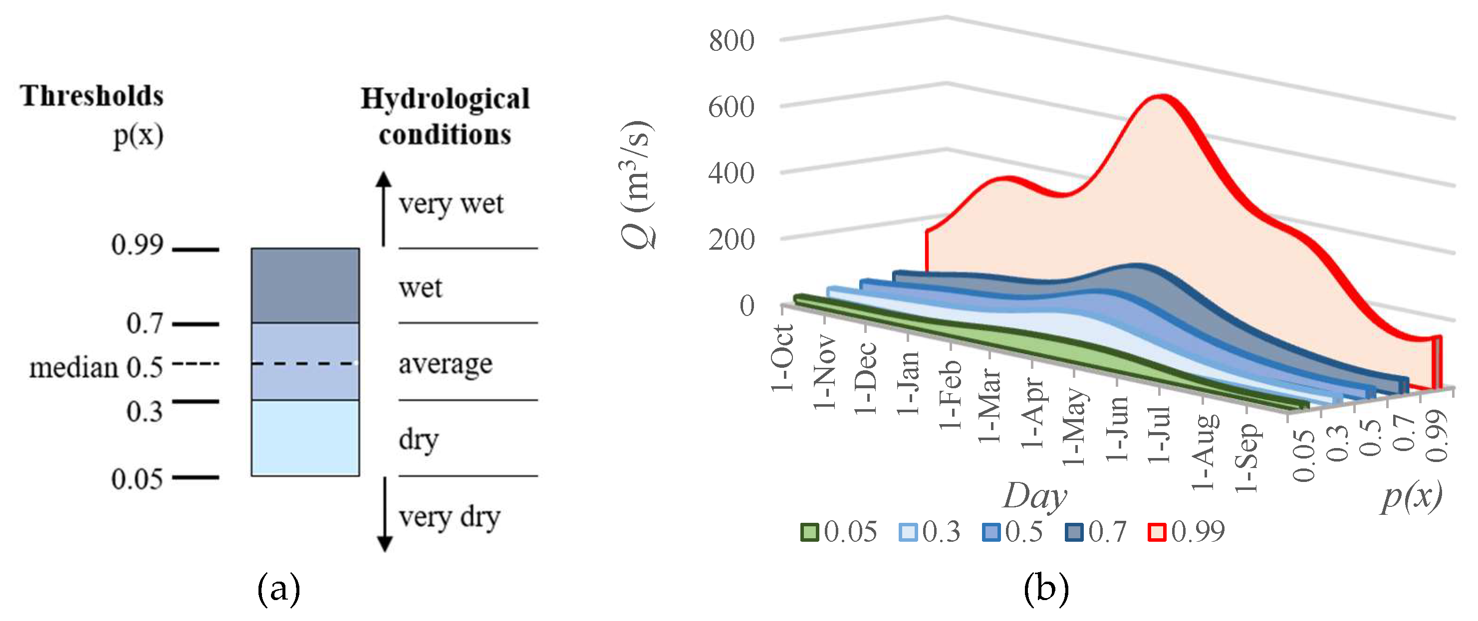
Hydrological condition zones are defined here for specific probabilities of occurrence of daily flows in the annual cycle. The zone thresholds, i.e., boundaries, are quantiles of specific probabilities (Figure 3a), selected to represent dry, average, and wet conditions, based on the previous research [3,7,23,36,40]. The average condition zone is the interval between the 0.3 and 0.7 quantiles. This zone is divided into two subzones by the median flow, p(x) = 0.5, an important hydrological indicator recommended by WMO as a measure of central tendency when undertaking assessments that focus on characterizing typical conditions [2]. The 0.05 quantile delineates the dry condition zone from the lowest zone representing extremely dry conditions, while the 0.99 quantile delineates the wet condition zone from the upper zone representing extremely wet conditions.
Runoff volumes corresponding to different hydrologic conditions are computed by integrating the area under the MDDF quantile line representing the upper boundary of that zone, as shown in Figure 3b.

3.5. Estimating Change in Hydrological Regime

The changes in seasonal runoff patterns are first examined visually by comparing the average zone and the median threshold (Figure 3a), as well as the periodical function of the mean daily flows. The changes in the annual and seasonal runoff volumes and timing between the two periods are computed by examining the area below the upper threshold of the hydrologic condition zone. The runoff volume is obtained by integrating this area (i.e., the flows representing specific MDDF quantiles), while the timing is described by the time coordinate of the centroid of this area [6,26]. The following two indicators of change are computed at annual and seasonal scales:
  • Relative change in runoff volume, ∆Vp (%):
    V p = V p 1991 2020 V p 1961 1991 V p 1961 1991 · 100
    where Vp is runoff volume below the p-th MDDF quantile representing the upper threshold of the zone for the given period.
  • Time shift of the centroid of the area below the MDDF quantile line, ∆t (in days):
    t = C p 1991 2020 C p 1961 1990
    where Cp is the time coordinate (ordinal number of day within year) of the centroid of the area under the p-th MDDF quantile for the given period.
The seasons within the hydrological year used for evaluation of the changes are defined as follows: October, November, and December represent autumn, January, February, and March—winter, April, May, and June—spring, and July, August, and September—summer.

4. Results

4.1. Daily Flow Statistics and Their Periodicity

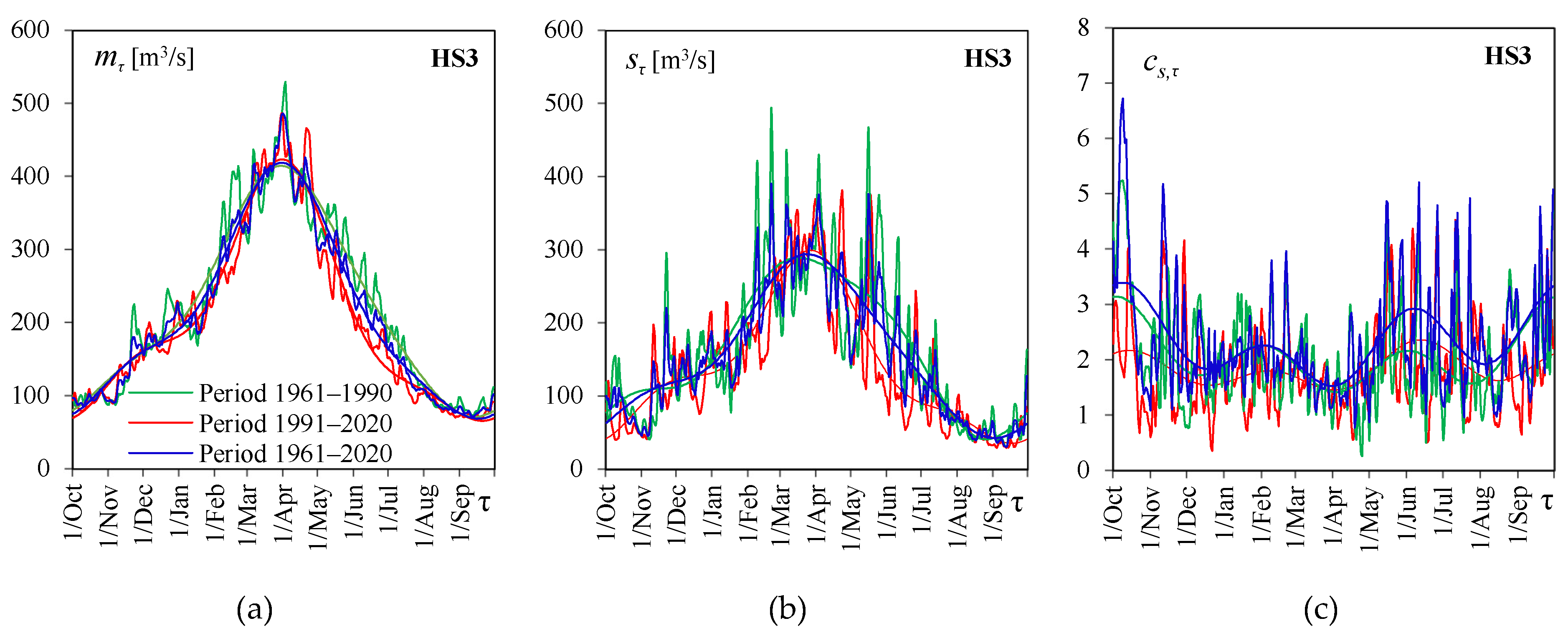
The daily statistics computed for each day within a year include the mean (mτ), standard deviation (sτ), and coefficient of skewness (c). Figure 4 shows the seasonal variation in the daily statistics for HS3 in all three considered periods, together with their corresponding periodic functions (smooth lines). The mean and standard deviation both exhibit distinct seasonal patterns which agree in phase. The highs occur in the spring and the lows in the summer (Figure 4a,b). This pattern is characteristic for all but two considered stations (HS1 and HS6). The skewness does not exhibit a distinct seasonal pattern like the mean and standard deviation, but a complex one with more highs and lows. It is also worth noting that there is a significant positive skewness over the entire annual cycle at all stations, as shown for HS3 in Figure 4c.
Figure 5 shows the daily statistics of the log-transformed data at HS3: mean (m), standard deviation (s), and skewness (csyτ), as well as their corresponding periodic functions. Expectedly, logarithmic transformation suppresses the variability in the daily statistics compared with the ones in the original space. The distinct seasonal pattern is still visible for the mean, but not for the standard deviation, for which the amplitude of the intra-annual oscillation is significantly smaller. The logarithmic transformation reduced the skewness and even produced negative values in both the daily skewness series and the estimated periodic function during certain parts of the year. This was noticed at all stations in some part of the year for at least one period considered. This further affects the parameters and the shape of the LPT3 marginal distributions. The statistics and their periodic functions for all stations are given in the Supplementary Materials (Figures S1 and S2).

4.2. Periodic Parameters of the Marginal LPT3 Distributions

The parameters of marginal LPT3 distributions are periodic functions, resulting from the periodic statistics myτ,per, syτ,per, and csyτ,per. Figure 6 shows the seasonal variation in the three LPT3 distribution parameters at HS3. The LPT3 parameters highly depend on the value and sign of the skew, csy. Therefore, a comparison of periodical functions of statistics (Figure 5) with LPT3 distribution parameters (Figure 6) expectedly shows that the differences between studied periods are transferred from the statistics (especially the skew) to the distribution parameters in accordance with the expressions in Equation (8). The results for all stations are given in the Supplementary Materials (Figure S3).

4.3. Marginal Distributions of Daily Flows

The flow quantiles Qpτ of a non-exceedance probability p = p(x) are estimated from the 365 fitted LPT3 distributions, one per each day within a year, with its periodic parameters. The smooth lines shown in Figure 7 represent the quantiles of MDDFs for the three periods considered at HS3. The results for all stations are given in the Supplementary Materials (Figure S4).
In general, the patterns of MDDFs in Figure 7 are defined by the periodic function of the mean (Figure 4a). The periodic functions of standard deviation (Figure 4b) and skew (Figure 4c) influence the spread and skewness of the annual MDDFs, respectively. Despite the peaky pattern for ατ,per and γ τ,per (Figure 6), the MDDF quantiles are represented by smooth lines. For days with a negative skew of log-transformed data (csyτ,per < 0) for 1961–1990 (green line in Figure 5c), marginal LPT3 distributions are bounded from above (Equation (9), also, e.g., [42]). The values of the upper bound were computed for all such cases and it was found that they do not cause underestimation of daily flow upper-tail quantiles for any non-exceedance probability of interest in hydrologic applications.
Visual inspection of the MDDFs in Figure 7 reveals that the differences between the three periods are the smallest for the median daily flows and in the average zone, and grow larger for the upper and lower quantiles. For this station, HS3, the maximum quantiles for 1991–2020 are higher and occur later compared with those for 1961–1990. For the joint 1961–2020 period, the quantile lines lie expectedly between the lines of the two subperiods.

4.4. The Zones of Hydrological Conditions

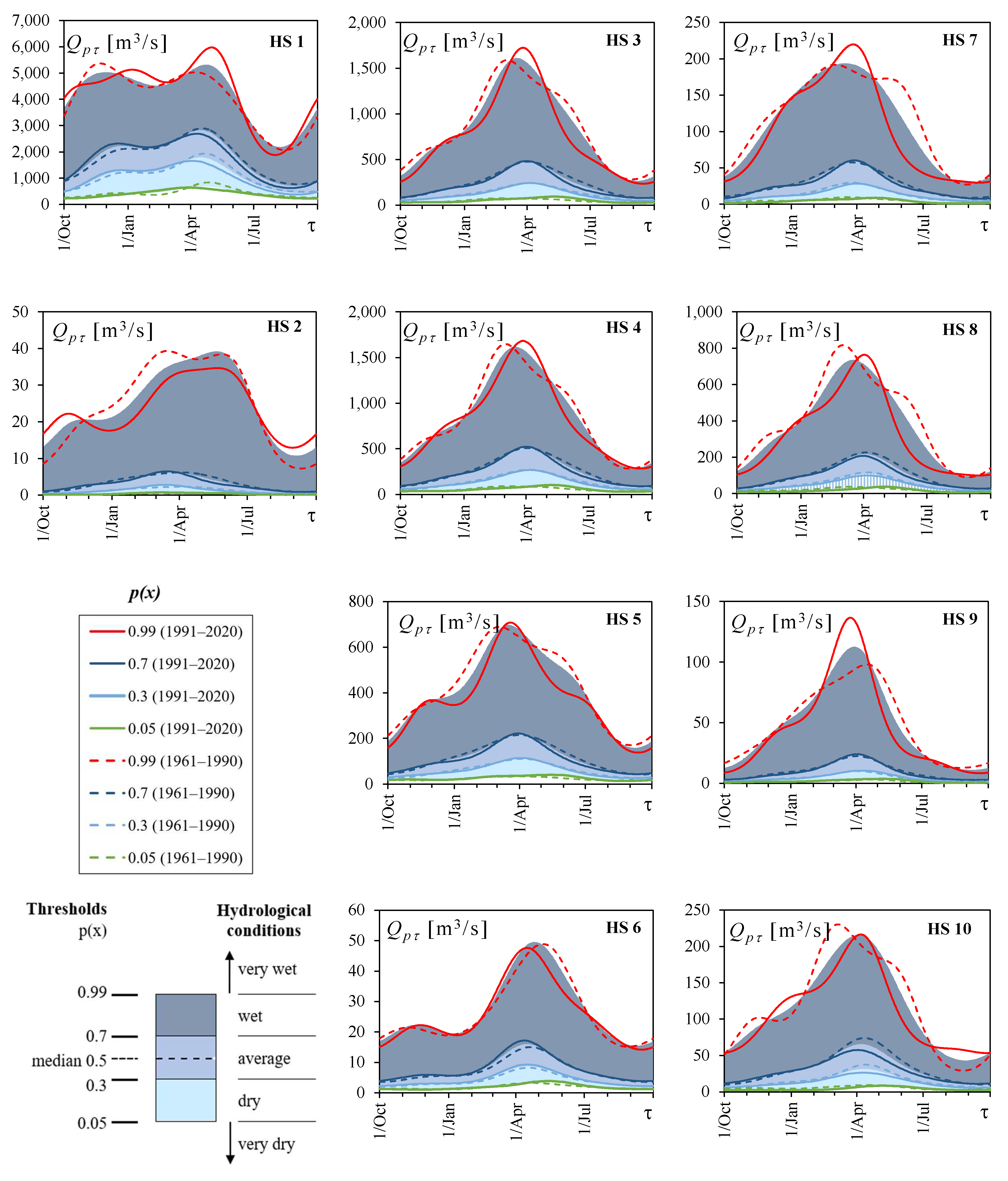
The zones of hydrological conditions for all stations are shown in Figure 8 in accordance with the adopted classification.
The patterns of thresholds (quantile lines) in Figure 8 obviously change with the period. The changes occurring in the wet condition zone at all stations are more visible due to the scale, but the changes in the dry condition zone are also significant, as can be seen in Figure 7b. At all stations, the pattern remains the same for quantiles 0.3, 0.5, and 0.7, which define the normal hydrological conditions. The seasonal pattern is not changed at any station from a simple unimodal shape to a mixed bimodal shape, or vice versa. The bimodal shape of the seasonal pattern is the most visible at HS1, where the most interesting change is for the 0.99 quantiles. Here, the primary peak in 1961–1990 was in the autumn while the secondary one was in the spring; in 1991–2020, the primary peak was in spring, while the secondary was in winter.

4.5. Annual and Seasonal Hydrologic Condition Changes

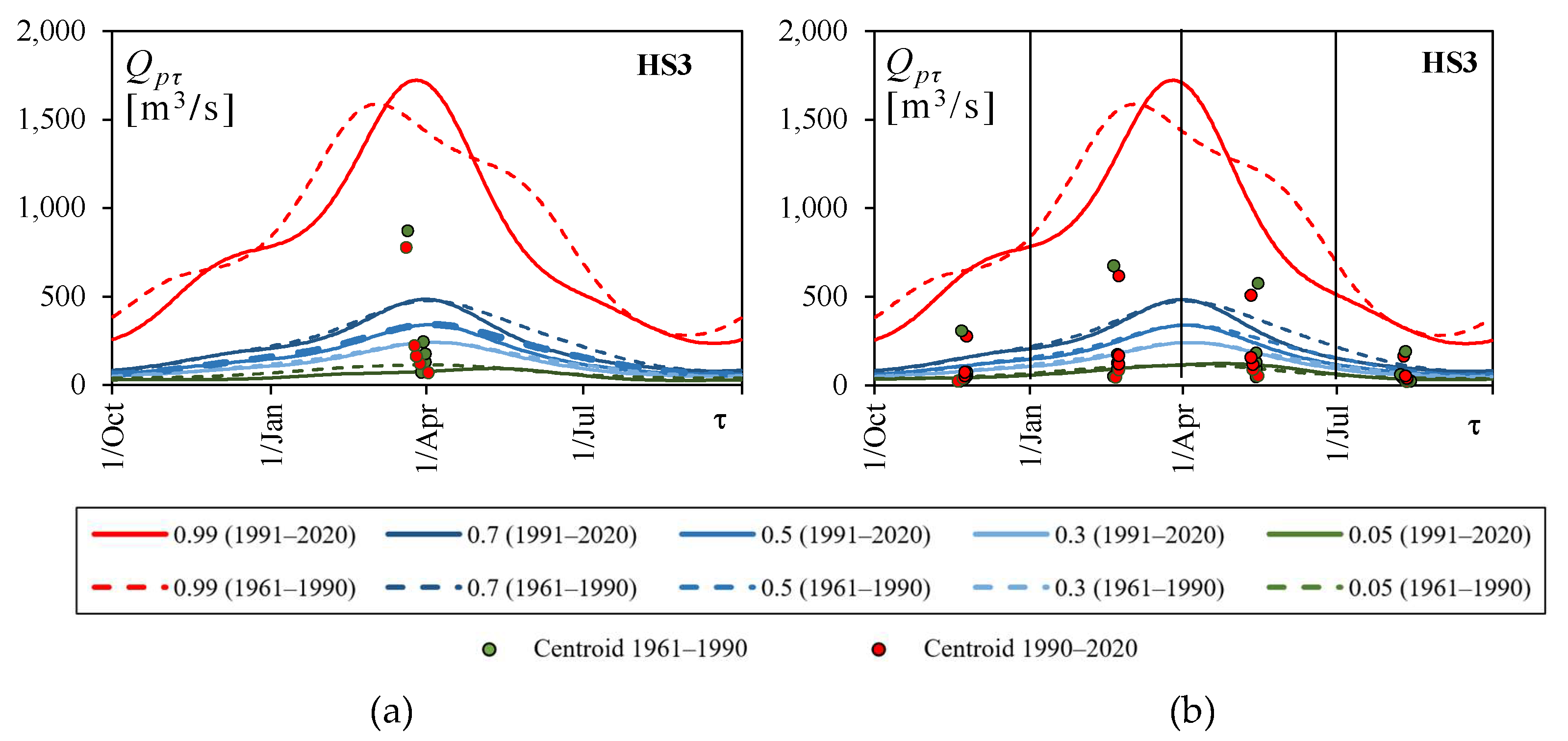
The graphical presentation of hydrologic condition zones defined in Figure 3a is helpful for detecting changes in daily flow patterns, while the quantification of change in respect to runoff timing and volume (the areas defined in Figure 3b) is required for practical purposes. Change in runoff timing is assessed from the shifts of the centroids of the areas below the upper thresholds of the hydrologic condition zones, as shown in Figure 9a for the annual scale and in Figure 9b for the seasonal scale at HS3.
Relative changes in runoff volume and time shifts of the centroids, calculated from Equations (10) and (11), are shown in Table 2 and Table 3, respectively, for all stations.
A general impression from Table 2 is that there is less runoff volume in the recent 30-year period compared with the previous one. HS6 is the only station at which runoff volume has increased in the recent period. HS2 and HS9 have distinct increases in extremely dry conditions in the winter and spring seasons, respectively. Additionally, HS2 exhibits a significant runoff volume increase in the wet condition zone in summer, as does HS10. The most unfavorable changes are found in HS10, with significant volume reductions in dry condition zones both annually and seasonally, and in all hydrologic condition zones in the spring. This station is located approximately 90 km downstream of the outflow of the Pirot hydropower plant (HPP) that started operation in 1990, at the very end of the first 30-year study period, as a peaking HPP [43]. It should be noted that we did not detect a change in the mean annual flow series of HS10 in the data preparation phase. This is most likely due to the small effect of this HPP and its reservoir on the regime of the downstream HS10 for several reasons: the small drainage area of the reservoir compared with the drainage area of HS10, the annual water balancing mode of the reservoir, and subdaily disturbance of the regime at HS10 by HPP outflows.
The shift in runoff timing shown in Table 3 is less pronounced compared with the relative volume change. The changes in more than 7 or 10 days might be significant for some applications in the water sector such as irrigation and hydropower operation planning. In that respect, the most significant changes are found at the annual scale in the dry and average condition zones in HS1 and HS2 of the Sava River basin, where the runoff centroids occur up to 11 and 8 days earlier, respectively. A later occurrence of dry conditions is found at the annual scale in HS7, HS8, and HS10, which are all situated in the upper and middle parts of the Južna Morava River basin. Wet hydrologic conditions occur 7 days later in HS2 and HS7 in summer, and 9 and 8 days earlier in HS7 and HS8, respectively, in the spring season.
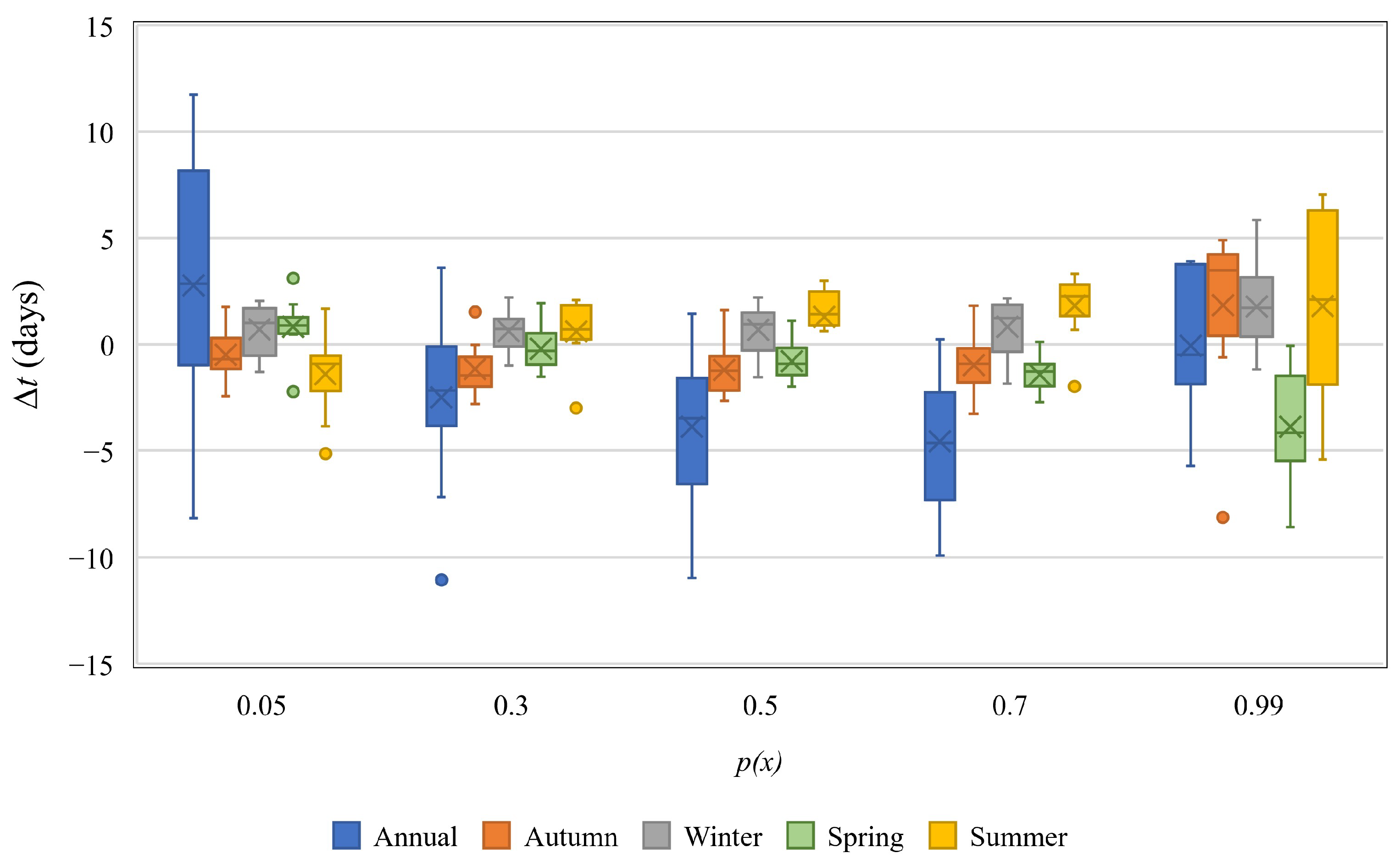
The data from Table 2 and Table 3 are shown as boxplots in Figure 10 and Figure 11, respectively. The results are organized in such a way that annual and seasonal changes in the hydrologic condition zones are easily grasped for the whole study area.
A general decreasing tendency in annual runoff volume in 1991–2020 compared with 1961–1990 at all stations is clearly visible from the boxplot in Figure 10. The most pronounced decrease is for the wet condition zone. Runoff volume has also decreased in all seasons and for all hydrological condition zones, except the autumn runoff in the average zone (for the 0.5 and 0.7 quantiles), and the spring runoff in the extremely dry zone. There is less water available in wet zones (0.7 to 0.99 quantiles) during the high-flow season in winter and spring. Similarly, in dry zones (0.3 and 0.05 quantiles) there is less water available in the summer and autumn seasons in the recent period 1991–2020.
In terms of runoff timing at the annual level (Figure 11), the centroids for dry and average conditions occur earlier in 1991–2020 compared with 1961–1990, while the centroids for wet conditions occur somewhat later. The seasonal changes in timing are not pronounced for all zones, but the centroids for wet conditions appear earlier in spring at all stations, and later in winter at most stations.
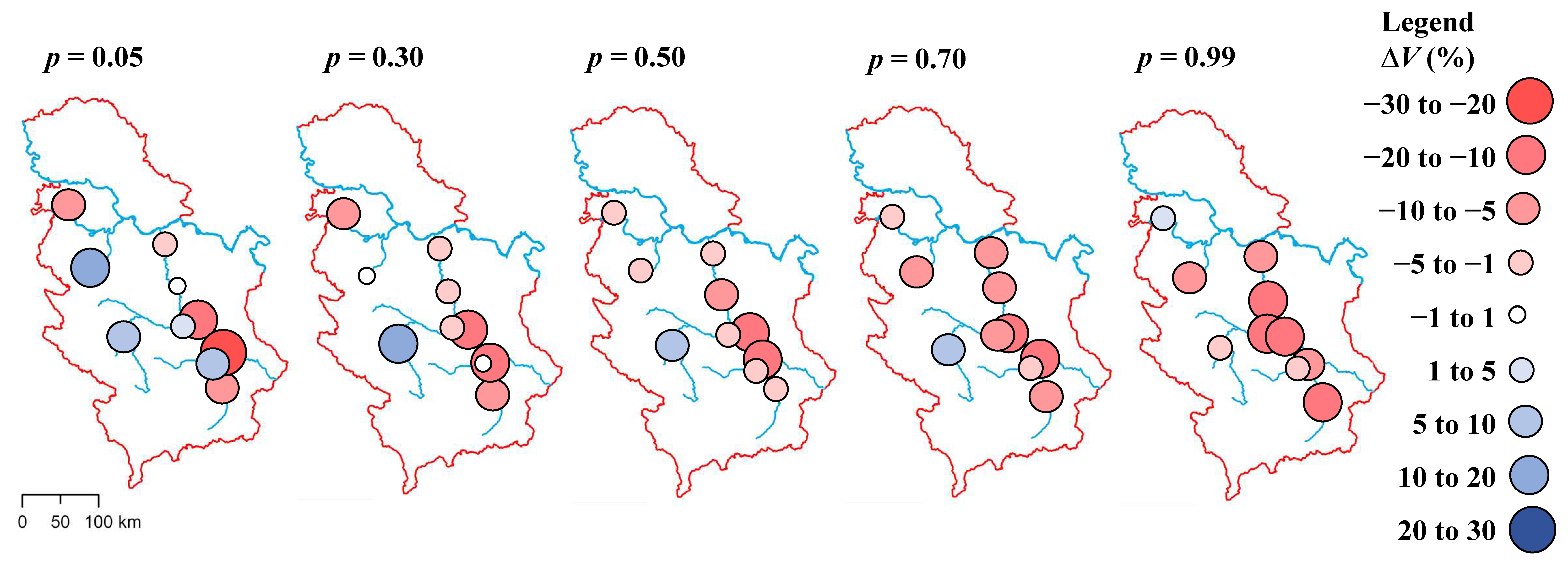
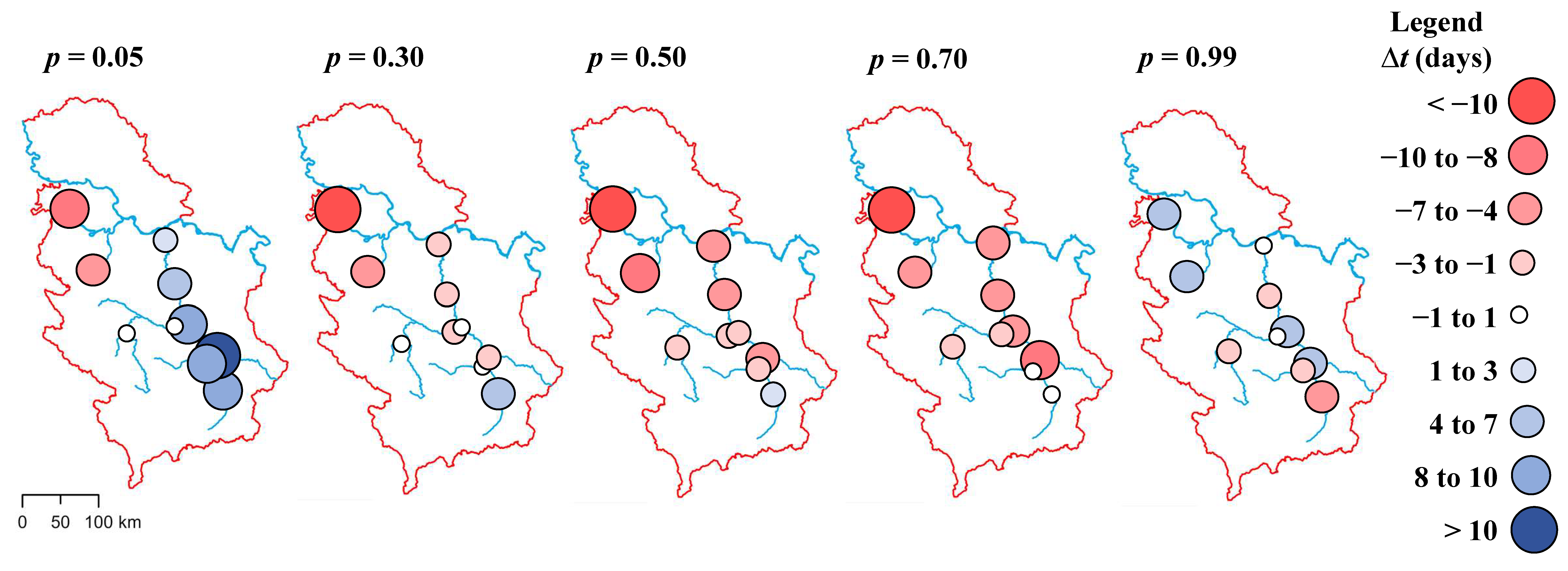
The annual changes in both runoff volume and runoff timing at all stations are mapped for spatial analysis in Figure 12 and Figure 13, respectively.
The spatial distribution of the relative volume change between the two periods shown in Figure 12 reveals that the catchments in western Serbia have experienced an increase in runoff volume in the recent period for the dry condition zone. It should be noted that these catchments are small to medium areas in size. The decrease in annual runoff volume is more pronounced at the transition from the average to wet condition zone in all catchments. The most western station, HS1, behaves differently compared with the other stations. It has the largest catchment area and represents the only station with runoff generated almost completely out of the country. This difference in behavior is pronounced in respect to runoff timing, as shown in Figure 13. The runoff timing for extreme dry conditions is later in the recent period at the annual level for all other stations. For the average wetness conditions, runoff generally occurs earlier, but this change is insignificant, while it generally occurs a bit later for wet conditions. The most southern station, HS7, shows earlier runoff timing for wet conditions. Expectedly, the timing shifts at the annual level are more pronounced compared with the shifts within seasons.

5. Discussion

5.1. Long-Term Changes in Hydrological Regime

The majority of previous studies considering the same area used trend detection of annual/seasonal/extreme flows to study hydrologic change in the past or in the future, or the “climate-hydrology-assessment chain” approach [44], in which a selected climate scenario plays an important role. Comparison of the approach presented here with other studies can therefore only be made indirectly, i.e., based on the detected changes. The methodology presented here can be used to analyze the seasonal runoff pattern, but it is less convenient for the analyses of phenomena at short, event-based time scales (such as flow flashiness) or at time scales longer than one year (such as interannual variability), as underlined by Blum et al. [36]. The probabilistic seasonal runoff pattern obtained from the MDDFs is used here to define zones of different hydrologic conditions and to detect a change in this pattern by looking into the changes in runoff timing and volume between the two 30-year periods. Our study is therefore aimed at detecting a structural change in the hydrological regime instead of the simple detection of trends or projections via climate change scenarios. The proposed approach is also not aimed at detecting the changes in intensity and frequency of flood events, which are often considered important consequences of climate change. However, our approach can be useful for a general understanding of the hydrological regime at a given location and can provide indications of the changes in the high-water regime, which is related to the floods.
In general, our results are consistent with the findings of Blöschl et al. [45], who reported decreasing flows in the Balkan region, and with Lobanova et al. [46], who used hydrologic simulations with a daily timestep under future climate conditions and concluded that shifts in runoff seasonality, particularly earlier occurrence of high flows in the snowmelt-driven catchments, can be expected. Also, according to [46], winter and early spring runoff in Central and Eastern Europe (in the high-flow season) are expected to increase. This is fairly consistent with our results (Figure 9), which show an increase in runoff in the wet season over 1991–2020 that is not significant (yet), but later timing of winter runoff and earlier timing of spring runoff (Figure 10) are detected, indicating the shifts in the wet period projected for the future in [46].
In a comprehensive analysis of trends in mean annual and seasonal flows in Serbia over 1961–2010 [47], no trend in mean annual flows was detected at all stations used in our study except HS8 and HS10, for which moderate decreasing trends were found. This is not in agreement with our findings from the data preparation phase (Table A1 in Appendix A) on the absence of trends over the 1961–2020 period at all stations considered. On the other hand, we found the greatest negative changes in annual runoff volume at HS8 and HS10 for the 0.5 quantile zone (−10% and −15%, respectively; see Table 2). In the same zone, HS6 exhibits the highest positive change in annual runoff volume of 10%, while there was no trend detected at this station in [47]. These discrepancies may stem from the difference in the periods for analysis (1961–2010 in [47] vs. 1961–2020 in our study), because the additional 10 years in our study cover a wetter period in Serbia, including an extremely wet year, 2014 (also known for extreme floods). On the seasonal level, a low-significance positive trend is found in [47] in autumn and winter runoff at HS6, whereas we found changes in seasonal runoff volume of 11% and 15% for autumn and winter, respectively. Additionally, a moderate negative trend in spring runoff at HS10 was found in [47], while our results show a change in spring runoff volume of −25%. However, we detected several considerable seasonal changes exceeding 10%, both positive and negative, in the average condition zone, while these were not detected as trends in [47].
A variety of studies about different aspects of hydrologic change for the Sava River (e.g., [14,48,49,50]) are in line with our results for HS1, showing that the mean flow is slightly declining. Hydrologic simulations in [49] for the near future (2011–2041), which partially overlaps with the second period in our study, indicate changes consistent with our results about increases in winter runoff volume in all hydrologic condition zones. An increase in winter runoff at HS1 is also found as a weak (statistically insignificant) positive trend over the long period of 1928–2017 [48]. A substantial decrease in river flows expected in the spring and summer seasons [49] is also visible in our results for all zones except for wet condition zones. The analysis of long-term trends of climate drivers and assessment of runoff in [50] also shows declining runoff in the Sava River basin as a consequence of increased air temperature and evapotranspiration. General findings in [13] for HS1 and HS4 indicate decreasing trends in summer and autumn runoff, and mostly increasing trends in winter and spring runoff, which are partially in accordance with our results. Our study indicates that HS1 and HS4 exhibit decreases in spring runoff volume and an increase in autumn runoff volume for the 0.5 quantile zone.
The hydrologic projections for the Kolubara (HS2) and Toplica (HS9) catchments indicate a decrease in snow storage and a substantial decrease in runoff in 2001–2030 (near future) compared with 1961–1990 (baseline period) [51]. Our results do not show a substantial but rather a slight decrease in runoff volume in the average and wet zones, which is closer to the findings of Idrizović et al. [52] for HS9. In [51], the largest decrease in runoff at HS9 is associated with the spring season, which is in accordance with our results for the wet zone only. The flood flow series simulated in [51] indicate little change for HS9 and a small increase for HS2 in median annual maximum floods. Our results for the wet zone at the annual scale for HS9 are consistent with these results, and also with the results in [52]. The analyses in [51] additionally show that the future droughts are expected to be more frequent, to last longer, and to start earlier in the summer for both the HS2 and HS9 catchments. Judging by the combination of change in runoff volume and time shifts in the dry and extremely dry zones (Table 2 and Table 3, 0.05 and 0.3 quantile), runoff reduction in these zones is already evident, but the time shift toward an earlier date can be seen in the extremely dry zone at HS9 only.

5.2. Probabilistic Annual Runoff Cycle as an Indicator of Hydrological Conditions

The probabilistic annual runoff cycle obtained from the MDDFs is used in this study to assess the changes over time in hydrological regime at selected rivers and locations in Serbia. It can also be used for other purposes, including operational monitoring of the hydrological regime aimed at early warnings and water management, and especially in operational reservoir management and management of droughts. The diagram with the MDDF of the annual runoff cycle (Figure 7) shows the zones of different hydrological conditions. Plotting actual hydrological data over this diagram clearly indicates current conditions in the catchment, but it can also reveal departures from normal conditions and anomalies. It can therefore be a support for responding to unfavorable situations and their mitigation.
The zones of hydrological conditions in the probabilistic annual runoff cycle are delimited by different probabilistic thresholds, which vary over the annual cycle because they represent the quantiles of MDDFs. This type of zoning based on probabilistic thresholds is very similar to the application of the SPI and SSI as drought indicators [29,30]. The main rationale behind the SPI and SSI as nondimensional (standardized) probabilistic indicators is to enable comparative analyses of precipitation or streamflow at different locations and at different times. Application of these two indices in monitoring hydrological conditions therefore requires the transformation of current precipitation or streamflow observations into standardized values. Contrary to this, the probabilistic annual runoff cycle allows direct evaluation of current streamflow observations for a given location.
A common characteristic of the methodologies for assessing the probabilistic annual runoff cycle and the SPI/SSI is related to fitting probability distributions to the observations. The SPI and SSI are usually calculated from monthly data over different accumulation periods from 1 to 12 months, whereas precipitation or streamflow accumulations for each month in a year are fitted by separate parametric or nonparametric distributions. Stagge et al. [33] attempted to fit a set of 365 parametric probability distributions for daily SPI estimation, but they retained the monthly averaging period. When compared with the SPI/SSI applications, using the daily time scale for the probabilistic annual runoff cycle provides information on runoff conditions with finer resolution and helps to avoid discontinuities when using the monthly scale and transiting from one month to another.
Regardless of temporal resolution, finding appropriate distribution type(s) for precipitation or streamflow is a crucial issue because it can considerably affect the computed SPI/SSI series and the derived drought characteristics [30,53]. Inappropriate distribution can lead to inconsistencies in the SPI or SSI such as the average not being equal to 0 and the variance not being equal to 1 [30]. When assessing the probabilistic annual runoff cycle for a given location, finding the most appropriate distribution is still a great challenge, but the targets of this process are less demanding regarding spatial comparability and in terms of constraints related to statistical properties.
Furthermore, the probabilistic annual runoff cycle is obtained here using the periodic functions for statistical properties of daily streamflow. This approach leads to smooth periodic-like lines of streamflow quantiles within a year and additionally ensures continuity of the thresholds that delineate certain hydrological condition zones.
As the SPI and SSI are devised as indices that should facilitate comparability of conditions in space and time, relevant thresholds that define specific conditions (e.g., droughts) are obtained via the equiprobability transformation from a selected distribution into the standardized normal quantiles. Typical thresholds are SPI = 0 or SSI = 0, and they are constant over the annual cycle. Conversely, the thresholds in the probabilistic annual runoff cycle are expressed directly in the physical units of streamflow at a given location and are therefore variable throughout a year. This provides a more intuitive presentation of the hydrological conditions in the annual cycle, and the zones delimited by these thresholds readily show deficits and surpluses in available water quantities.

6. Conclusions

Hydrologic change detection involves different identification approaches, temporal scales, and spatial scales. This study presents an analysis of changes in the annual and seasonal runoff of ten catchments in Serbia in the 1961–2020 period at the daily time scale. The analysis is based on the probabilistic representation of the seasonal runoff pattern that is obtained from marginal distributions of daily flows (MDDFs) with periodic distribution parameters inherited from the periodic statistical parameters of daily flow series. The hydrologic (wetness) conditions are defined as the zones between the MDDF quantiles of specific probabilities, selected to depict dry, average, and wet normal conditions in the catchment.
Based on a comparison of these zones between the two 30-year periods at the annual and seasonal scales, the following may be concluded:
  • The seasonal runoff pattern changed from one period to another in terms of temporal shift and the occurrence of more extreme flows. However, the general pattern of seasonal runoff remained the same. The prevailing pattern is simple and unimodal, while the less present mixed regime is bimodal.
  • In most of the catchments, runoff volume has decreased in the recent 1991–2020 period at both the annual and seasonal scales. The critical season is summer for dry and average conditions, with volume reduction in all catchments.
  • The most pronounced shift in runoff timing is found on the annual scale. Dry and average conditions occur earlier at this scale. The change in runoff timing is found to be insignificant for all seasons and zones, except for wet conditions, which occur earlier in spring.
The proposed zoning of hydrologic conditions based on probabilistic variable daily flow thresholds enables more precise analysis of runoff volume and timing between the selected periods. It also enables more detailed analysis of zones that are critical for some applications in a certain period of the year. For instance, such an analysis may be of interest in drought-related studies in the seasons when water deficit conflicts with water demand.
The results of this study are generally in line with the results of the previous hydrologic change analyses in the study area, in terms of both past changes and those predicted for the near-future climate, but our results may be considered more detailed due to the applied approach based on MDDFs with periodic distribution parameters. It is demonstrated that the proposed approach allows for detecting a structural change in the hydrological regime, and detecting changes in the regulated flow regime when statistical tests cannot detect the change. The daily time scale of the seasonal runoff pattern representation makes this approach more useful for monitoring actual catchment wetness and runoff conditions and therefore for operational water management and early warning systems. In situational assessment and forecasting, the wetness condition zones may be used for flow forecasting by focusing on the zone to which current daily flows belong. It is worth noting that the boundaries of the wetness zones could be changed easily depending on the purpose required. Furthermore, the zone boundaries, i.e., the probabilistic thresholds, can also be converted to hydrologic drought indicators such as the SSI.

Supplementary Materials

The following supporting information can be downloaded at https://www.mdpi.com/article/10.3390/w15162919/s1. Figure S1: Seasonal variation of daily flow statistics (peaky lines) and their corresponding periodic functions (smooth lines) at all HS estimated for the three periods: (a) mean, (b) standard deviation, and (c) coefficient of skewness; Figure S2: Seasonal variation of log-transformed daily flow statistics (peaky lines) and their corresponding periodic functions (smooth lines) at all HS estimated for the three periods: (a) mean, (b) standard deviation, and (c) coefficient of skewness; Figure S3: Periodical parameters of LPT3 marginal distribution of daily flows at all HS: (a) shape parameter ατ,per, (b) scale parameter βτ,per, (c) location parameter γ τ,per; Figure S4: The diagrams of MDDF at all HS for the three periods showing the quantiles (a) for a full range of probabilities p(x), from 0.01 to 0.99, and (b) for low to median probabilities. Solid lines represent the latest 1991–2020 period, the dashed lines represent the earlier 1961–1990 period, and the dotted lines represent the whole 1961–2020 period.

Author Contributions

Conceptualization, B.B. and V.M.; methodology, B.B. and V.M.; validation, B.B., V.M. and A.B.; formal analysis, B.B., V.M., A.B. and J.P.; investigation, B.B., V.M. and A.B.; data curation, V.M. and A.B.; writing—original draft preparation, B.B., V.M. and J.P.; visualization, V.M. and B.B.; funding acquisition, B.B., V.M. and J.P. All authors have read and agreed to the published version of the manuscript.

Funding

This research was partially funded by the Ministry of Education, Science and Techno-logical Development of the Republic of Serbia, grant numbers 451-03-47/2023-01/200095, 451-03-47/2023-01/200169, and 451-03-47/2023-01/200092.

Data Availability Statement

The data are not publicly available because they are owned by the Republic Hydrometeorological Service of Serbia.

Acknowledgments

The authors would like to thank the Republic Hydrometeorological Service of Serbia for the provision of data. The authors would like to acknowledge the initial support to the research of the late Ass. Prof. Dr. Zoran M. Radić from the University of Belgrade—Faculty of Civil Engineering, Serbia.

Conflicts of Interest

The authors declare no conflict of interest.

Appendix A

Table A1 shows the results of statistical tests for the homogeneity, randomness, and trends of annual flows at the 10 hydrological stations used in this study over the 1961–2020 period. The table shows p-values of the test statistics in the following tests: a test on the difference between two means (Z-test), two tests on the difference between two variances (Fisher’s F-test and Levene’s test), the Mann–Whitney test for homogeneity, the Wald–Wolfowitz run test for independence, and the Mann–Kendall test for trends (with the null hypothesis that there is no trend in the data).
Table A1. Results (p-values) of the tests applied to the annual flow series for the period 1961–2020.
HS#Z 1F 2L 3M-W 4W-W 5M-K 6
10.7920.8880.9460.7920.5200.444
20.5070.4690.7320.5840.3670.329
30.1500.4300.5630.0920.8990.211
40.4020.3440.4420.3820.7000.506
50.2060.8090.4200.1520.8960.367
60.3740.6730.6190.3930.0530.415
70.3580.0890.2150.1840.5200.255
80.1110.7290.7930.0840.3670.154
90.2540.9680.5880.2620.5200.293
100.6010.6540.3900.5160.7000.354
Note(s): 1 Z-test; 2 Fisher’s F-test; 3 Levene’s test; 4 Mann–Whitney test; 5 Wald–Wolfowitz test; 6 Mann–Kendall test.

References

  1. Bridgewater, P.; Guarino, E.; Thompson, R.M. Hydrology in the Anthropocene. In Encyclopedia of the Anthropocene; Elsevier: Amsterdam, The Netherlands, 2017; Volume 1–5, pp. 87–92. ISBN 9780128096659. [Google Scholar]
  2. WMO Hydrological Coordination Panel. Statement on the Term Hydrological Normal. Available online: https://community.wmo.int/en/activity-areas/hydrology-and-water-resources/hydrological-coordination-panel (accessed on 13 June 2023).
  3. Pekarova, P.; Gorbachova, L.; Mitkova, V.B.; Pekar, J.; Miklanek, P. Statistical Analysis of Hydrological Regime of the Danube River at Ceatal Izmail Station. IOP Conf. Ser. Earth Environ. Sci. 2019, 221, 012035. [Google Scholar] [CrossRef]
  4. Renner, M.; Bernhofer, C. Long Term Variability of the Annual Hydrological Regime and Sensitivity to Temperature Phase Shifts in Saxony/Germany. Hydrol. Earth Syst. Sci. 2011, 15, 1819–1833. [Google Scholar] [CrossRef] [Green Version]
  5. Plavšić, J.; Milutinović, R. O računskim nivoima vode za zaštitu od poplava na Dunavu kod Novog Sada. Vodoprivreda 2010, 42, 69–78. [Google Scholar]
  6. Stewart, I.T.; Cayan, D.R.; Dettinger, M.D. Changes toward Earlier Streamflow Timing across Western North America. J. Clim. 2005, 18, 1136–1155. [Google Scholar] [CrossRef]
  7. Laaha, G.; Blöschl, G. Seasonality Indices for Regionalizing Low Flows. Hydrol. Process. 2006, 20, 3851–3878. [Google Scholar] [CrossRef] [Green Version]
  8. Eisner, S.; Flörke, M.; Chamorro, A.; Daggupati, P.; Donnelly, C.; Huang, J.; Hundecha, Y.; Koch, H.; Kalugin, A.; Krylenko, I.; et al. An Ensemble Analysis of Climate Change Impacts on Streamflow Seasonality across 11 Large River Basins. Clim. Chang. 2017, 141, 401–417. [Google Scholar] [CrossRef]
  9. Poschlod, B.; Willkofer, F.; Ludwig, R. Impact of Climate Change on the Hydrological Regimes in Bavaria. Water 2020, 12, 1599. [Google Scholar] [CrossRef]
  10. Yeste, P.; Rosa-Cánovas, J.J.; Romero-Jiménez, E.; García-Valdecasas Ojeda, M.; Gámiz-Fortis, S.R.; Castro-Díez, Y.; Esteban-Parra, M.J. Projected Hydrologic Changes over the North of the Iberian Peninsula Using a Euro-CORDEX Multi-Model Ensemble. Sci. Total Environ. 2021, 777, 146126. [Google Scholar] [CrossRef]
  11. Hobeichi, S.; Abramowitz, G.; Ukkola, A.M.; De Kauwe, M.; Pitman, A.; Evans, J.P.; Beck, H. Reconciling Historical Changes in the Hydrological Cycle over Land. NPJ Clim. Atmos. Sci. 2022, 5, 17. [Google Scholar] [CrossRef]
  12. Brunner, M.I.; Melsen, L.A.; Newman, A.J.; Wood, A.W.; Clark, M.P. Future Streamflow Regime Changes in the United States: Assessment Using Functional Classification. Hydrol. Earth Syst. Sci. 2020, 24, 3951–3966. [Google Scholar] [CrossRef]
  13. Stojković, M.; Plavšić, J.; Prohaska, S. Dugoročne promene godišnjih i sezonskih proticaja: Primer reke Save. Vodoprivreda 2014, 46, 39–48. [Google Scholar]
  14. Stojković, M.; Ilić, A.; Prohaska, S.; Plavšić, J. Multi-Temporal Analysis of Mean Annual and Seasonal Stream Flow Trends, Including Periodicity and Multiple Non-Linear Regression. Water Resour. Manag. 2014, 28, 4319–4335. [Google Scholar] [CrossRef]
  15. Kundzewicz, Z.W.; Robson, A. (Eds.) Detecting Trend and Other Changes in Hydrological Data; WMO/TD-No. 1013; World Meteorological Organization: Geneva, Switzerland, 2000.
  16. Hamed, K.H.; Ramachandra Rao, A. A Modified Mann-Kendall Trend Test for Autocorrelated Data. J. Hydrol. 1998, 204, 182–196. [Google Scholar] [CrossRef]
  17. Pettitt, A.N. A Non-Parametric Approach to the Change-Point Problem. Appl. Stat. 1979, 28, 126. [Google Scholar] [CrossRef]
  18. Zhang, A.; Zheng, C.; Wang, S.; Yao, Y. Analysis of Streamflow Variations in the Heihe River Basin, Northwest China: Trends, Abrupt Changes, Driving Factors and Ecological Influences. J. Hydrol. Reg. Stud. 2015, 3, 106–124. [Google Scholar] [CrossRef] [Green Version]
  19. Serinaldi, F.; Kilsby, C.G.; Lombardo, F. Untenable Nonstationarity: An Assessment of the Fitness for Purpose of Trend Tests in Hydrology. Adv. Water Resour. 2018, 111, 132–155. [Google Scholar] [CrossRef]
  20. Hannaford, J.; Buys, G.; Stahl, K.; Tallaksen, L.M. The Influence of Decadal-Scale Variability on Trends in Long European Streamflow Records. Hydrol. Earth Syst. Sci. 2013, 17, 2717–2733. [Google Scholar] [CrossRef] [Green Version]
  21. Stojković, M.; Prohaska, S.; Plavšić, J. Stochastic Structure of Annual Discharges of Large European Rivers. J. Hydrol. Hydromech. 2015, 63, 63–70. [Google Scholar] [CrossRef] [Green Version]
  22. Blöschl, G.; Sivapalan, M.; Wagener, T.; Viglione, A.; Savenije, H. (Eds.) Runoff Prediction in Ungauged Basins: Synthesis across Processes, Places and Scales; Cambridge University Press: Cambridge, UK, 2013; ISBN 978-1-107-02818-0. [Google Scholar]
  23. Salinas-Rodríguez, S.A.; Sánchez-Navarro, R.; Barrios-Ordóñez, J.E. Frequency of Occurrence of Flow Regime Components: A Hydrology-Based Approach for Environmental Flow Assessments and Water Allocation for the Environment. Hydrol. Sci. J. 2021, 66, 193–213. [Google Scholar] [CrossRef]
  24. Zeiringer, B.; Seliger, C.; Greimel, F.; Schmutz, S. River Hydrology, Flow Alteration, and Environmental Flow. In Riverine Ecosystem Management; Springer International Publishing: Cham, Switzerland, 2018; pp. 67–89. [Google Scholar]
  25. Cammalleri, C.; Vogt, J.; Salamon, P. Development of an Operational Low-Flow Index for Hydrological Drought Monitoring over Europe. Hydrol. Sci. J. 2016, 62, 346–358. [Google Scholar] [CrossRef] [Green Version]
  26. Mendoza, P.A.; Clark, M.P.; Mizukami, N.; Newman, A.J.; Barlage, M.; Gutmann, E.D.; Rasmussen, R.M.; Rajagopalan, B.; Brekke, L.D.; Arnold, J.R. Effects of Hydrologic Model Choice and Calibration on the Portrayal of Climate Change Impacts. J. Hydrometeorol. 2015, 16, 762–780. [Google Scholar] [CrossRef]
  27. Abdul Aziz, O.I.; Burn, D.H. Trends and Variability in the Hydrological Regime of the Mackenzie River Basin. J. Hydrol. 2006, 319, 282–294. [Google Scholar] [CrossRef]
  28. Fleig, A.K.; Tallaksen, L.M.; Hisdal, H.; Demuth, S. A Global Evaluation of Streamflow Drought Characteristics. Hydrol. Earth Syst. Sci. 2006, 10, 535–552. [Google Scholar] [CrossRef] [Green Version]
  29. McKee, T.B.; Doesken, N.J.; Kleist, J. The Relationship of Drought Frequency and Duration to Time Scales. In Proceedings of the 8th Conference on Applied Climatology, Anaheim, CA, USA, 17–22 January 1993; American Meteorological Society: Boston, MA, USA, 1993; pp. 179–183. [Google Scholar]
  30. Vicente-Serrano, S.M.; López-Moreno, J.I.; Beguería, S.; Lorenzo-Lacruz, J.; Azorin-Molina, C.; Morán-Tejeda, E. Accurate Computation of a Streamflow Drought Index. J. Hydrol. Eng. 2012, 17, 318–332. [Google Scholar] [CrossRef] [Green Version]
  31. Mihailović, V.; Blagojević, B. Izbor teorijske raspodele verovatnoća na osnovu L-momenata u proračunu pokazatelja meteorološke i hidrološke suše. Vodoprivreda 2015, 47, 273–278. [Google Scholar]
  32. Ozkaya, A.; Zerberg, Y. A 40-Year Analysis of the Hydrological Drought Index for the Tigris Basin, Turkey. Water 2019, 11, 657. [Google Scholar] [CrossRef] [Green Version]
  33. Stagge, J.H.; Tallaksen, L.M.; Gudmundsson, L.; Van Loon, A.F.; Stahl, K. Candidate Distributions for Climatological Drought Indices (SPI and SPEI). Int. J. Climatol. 2015, 35, 4027–4040. [Google Scholar] [CrossRef]
  34. Sutanto, S.J.; Van Lanen, H.A.J. Streamflow Drought: Implication of Drought Definitions and Its Application for Drought Forecasting. Hydrol. Earth Syst. Sci. 2021, 25, 3991–4023. [Google Scholar] [CrossRef]
  35. Yevjevich, V. Structure of Daily Hydrologic Series; Water Resources Publications: Littleton, CO, USA, 1984. [Google Scholar]
  36. Blum, A.G.; Archfield, S.A.; Vogel, R.M. On the Probability Distribution of Daily Streamflow in the United States. Hydrol. Earth Syst. Sci. 2017, 21, 3093–3103. [Google Scholar] [CrossRef] [Green Version]
  37. Yevjevich, V. Stochastic Processes in Hydrology; Water Resources Publications: Littleton, CO, USA, 1972. [Google Scholar]
  38. Radić, Z.; Mihailović, V. Marginalne raspodele dnevnih proticaja na reprezentativnim profilima u Srbiji. Vodoprivreda 2010, 42, 17–38. [Google Scholar]
  39. Mihailović, V. Složena Analiza Hidroloških Vremenskih Serija za Potrebe Modeliranja Ekstremnih Događaja (A Complex Analysis of Hydrological Time Series for Modelling Extreme Events). Doctoral Thesis, University of Belgrade—Faculty of Civil Engineering, Belgrade, Serbia, 2012. [Google Scholar]
  40. Hayes, D.S.; Brändle, J.M.; Seliger, C.; Zeiringer, B.; Ferreira, T.; Schmutz, S. Advancing towards Functional Environmental Flows for Temperate Floodplain Rivers. Sci. Total Environ. 2018, 633, 1089–1104. [Google Scholar] [CrossRef] [PubMed]
  41. Bogojević, A. Strukturna Analiza Serija Dnevnih Protoka u Profilima Hidroloških Stanica na Teritoriji Srbije (Structural Analysis of Daily Flow Series at Hydrological Stations in the Territory of Serbia). Bachelor’s Thesis, University of Niš, Faculty of Civil Engineering and Architecture, Niš, Serbia, 2022. [Google Scholar]
  42. Bobée, B.; Ashkar, F. The Gamma Family and Derived Distributions Applied in Hydrology; Water Resources Publications: Littleton, CO, USA, 1991; ISBN 978-0918334688. [Google Scholar]
  43. Elektroprivreda Srbije, HE Pirot. Available online: https://www.eps.rs/lat/djerdap/Stranice/he_pirot.aspx (accessed on 4 August 2023).
  44. Olsson, J.; Arheimer, B.; Borris, M.; Donnelly, C.; Foster, K.; Nikulin, G.; Persson, M.; Perttu, A.-M.; Uvo, C.; Viklander, M.; et al. Hydrological Climate Change Impact Assessment at Small and Large Scales: Key Messages from Recent Progress in Sweden. Climate 2016, 4, 39. [Google Scholar] [CrossRef] [Green Version]
  45. Blöschl, G.; Hall, J.; Viglione, A.; Perdigão, R.A.P.; Parajka, J.; Merz, B.; Lun, D.; Arheimer, B.; Aronica, G.T.; Bilibashi, A.; et al. Changing Climate Both Increases and Decreases European River Floods. Nature 2019, 573, 108–111. [Google Scholar] [CrossRef] [PubMed]
  46. Lobanova, A.; Liersch, S.; Nunes, J.P.; Didovets, I.; Stagl, J.; Huang, S.; Koch, H.; López, M.D.R.R.; Maule, C.F.; Hattermann, F.; et al. Hydrological Impacts of Moderate and High-End Climate Change across European River Basins. J. Hydrol. Reg. Stud. 2018, 18, 15–30. [Google Scholar] [CrossRef]
  47. Kovacevic-Majkic, J.; Urosev, M. Trends of Mean Annual and Seasonal Discharges of Rivers in Serbia. J. Geogr. Inst. Jovan Cvijic SASA 2014, 64, 143–160. [Google Scholar] [CrossRef]
  48. Leščešen, I.; Šraj, M.; Pantelić, M.; Dolinaj, D. Assessing the Impact of Climate on Annual and Seasonal Discharges at the Sremska Mitrovica Station on the Sava River, Serbia. Water Supply 2022, 22, 195–207. [Google Scholar] [CrossRef]
  49. The World Bank. Water and Climate Adaptation Plan for the Sava River Basin: Main Report; World Bank Group: Washington, DC, USA, 2015. Available online: https://www.savacommission.org/documents-and-publications/technical-and-project-reports/water-and-climate-adaptation-plan-for-the-sava-river-basin-watcap/245 (accessed on 13 June 2023).
  50. Pandžić, K.; Trninić, D.; Likso, T.; Bošnjak, T. Long-Term Variations in Water Balance Components for Croatia. Theor. Appl. Climatol. 2009, 95, 39–51. [Google Scholar] [CrossRef]
  51. Langsholt, E.; Lawrence, D.; Wong, W.K.; Andjelic, M.; Ivkovic, M.; Vujadinovic, M. Effects of Climate Change in The Kolubara and Toplica Catchments, Serbia; Haddeland, I., Ed.; Norwegian Water Resources and Energy Directorate: Oslo, Norway, 2013. [Google Scholar]
  52. Idrizovic, D.; Pocuca, V.; Vujadinovic Mandic, M.; Djurovic, N.; Matovic, G.; Gregoric, E. Impact of Climate Change on Water Resource Availability in a Mountainous Catchment: A Case Study of the Toplica River Catchment, Serbia. J. Hydrol. 2020, 587, 124992. [Google Scholar] [CrossRef]
  53. Tijdeman, E.; Stahl, K.; Tallaksen, L.M. Drought Characteristics Derived Based on the Standardized Streamflow Index: A Large Sample Comparison for Parametric and Nonparametric Methods. Water Resour. Res. 2020, 56, e2019WR026315. [Google Scholar] [CrossRef]
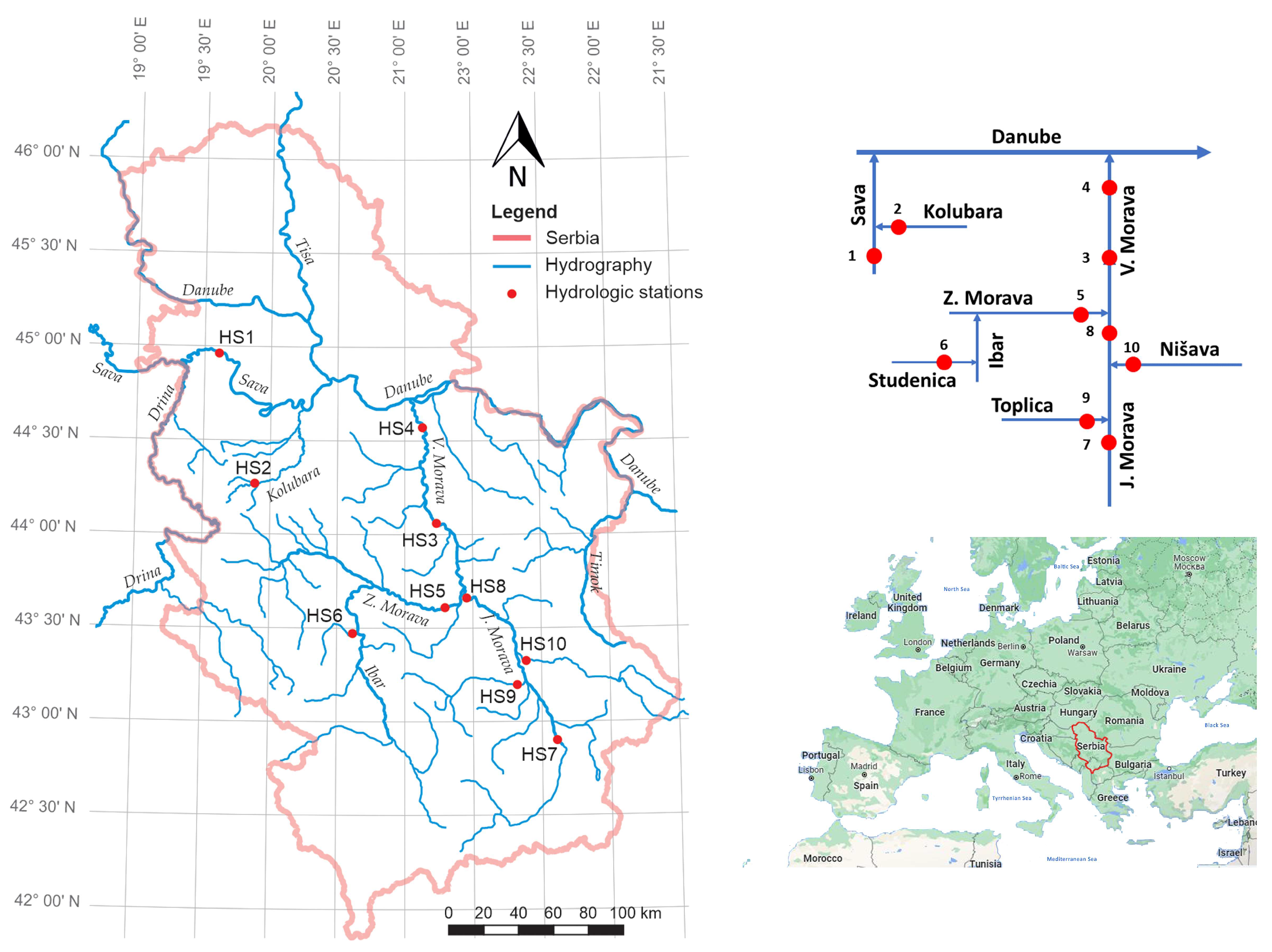
Figure 1. Locations of the hydrological stations used in this study on the hydrographic map of Serbia (left) and a schematic of the river network and stations (upper right panel).
Water 15 02919 g001
Figure 2. Illustration of methodological steps to detect changes in hydrological regime.
Water 15 02919 g002
Figure 3. Hydrological condition zones based on probabilistic threshold levels for (a) flows, (b) runoff volumes.
Water 15 02919 g003
Figure 4. Seasonal variation in daily flow statistics (peaky lines) and their corresponding periodic functions (smooth lines) at HS3 estimated for the three periods: (a) mean, (b) standard deviation, and (c) coefficient of skewness. Modified from [41].
Water 15 02919 g004
Figure 5. Seasonal variation in log-transformed daily flow statistics (peaky lines) and their corresponding periodic functions at HS3 estimated for the three periods: (a) mean, (b) standard deviation, and (c) coefficient of skewness. Modified from [41].
Water 15 02919 g005
Figure 6. Periodical parameters of LPT3 marginal distribution of daily flows at HS3: (a) shape parameter ατ,per, (b) scale parameter β τ,per, (c) location parameter γ τ,per. Modified from [41].
Water 15 02919 g006
Figure 7. The diagrams of MDDFs at HS3 for the three periods showing the quantiles (a) for a full range of probabilities p(x), from 0.01 to 0.99, and (b) for low to median probabilities. The solid lines represent the later 1991–2020 period, the dashed lines represent the earlier 1961–1990 period, and the dotted lines represent the whole 1961–2020 period.
Water 15 02919 g007
Figure 8. Hydrological condition zones for all stations defined by the quantiles of marginal daily flow distributions for selected probabilities. The zones for the 1961–2020 period are shaded, while the zones for two subperiods are indicated by their upper threshold lines.
Water 15 02919 g008
Figure 9. The centroids of the area below the upper thresholds of the hydrologic condition zones for (a) annual and (b) seasonal scales. Red dots refer to the recent 1991–2020 period, and green ones to the earlier 1961–1990 period.
Water 15 02919 g009
Figure 10. The boxplots of changes in the annual and seasonal runoff volumes in 1991–2020 compared with 1961–1990 at all stations for the wetness condition zones defined using the upper quantiles of probability p(x). The lines in the boxplots indicate the median value and x indicates the mean, while the whiskers correspond to 1.5 × IQR, where IQR is the interquartile range, with the outliers outside IQR displayed.
Water 15 02919 g010
Figure 11. The boxplots of changes in the annual and seasonal runoff timing in 1991–2020 compared with 1961–1990 at all stations for the wetness condition zones defined by the upper quantiles of probability p(x). The lines in the boxplot indicate the median value and x indicates the mean, while the whiskers correspond to 1.5 × IRQ, where IRQ is the interquartile range, with the outliers outside IQR displayed.
Water 15 02919 g011
Figure 12. The maps of relative change in annual runoff volume at ten stations for dry, average, and wet condition zones, represented by upper quantiles of probability p(x). Red circles denote volume reduction in 1991–2020 compared with 1961–1990, and blue circles indicate volume increase. The circle size corresponds to the amount of change.
Water 15 02919 g012
Figure 13. The maps of changes in timing of annual runoff at ten stations for dry, average, and wet condition zones, represented by upper quantiles of probability p(x). Red circles denote earlier runoff occurrence in 1991–2020 compared with 1961–1990, and blue circles indicate later timing. The circle size corresponds to the amount of change.
Water 15 02919 g013
Table 1. Hydrological stations (HS) used in this study.
HS#Station NameRiverCatchment Area [km2]Watershed
1Sremska MitrovicaSava87,996Sava
2ValjevoKolubara340Kolubara
3BagrdanVelika Morava33,446Velika Morava
4Ljubičevski mostVelika Morava37,320Velika Morava
5JasikaZapadna Morava14,721Zapadna Morava
6UšćeStudenica540ZapadnaMorava
7GrdelicaJužna Morava3782Južna Morava
8MojsinjeJužna Morava15,390Južna Morava
9DoljevacToplica2052Južna Morava
10NišNišava3870Južna Morava
Table 2. Relative change in runoff volume (%) in the recent 1991–2020 period compared with the 1961–1990 period. The first column indicates the probabilities p(x) of the upper thresholds of the hydrologic condition zones. Changes are shown for annual (Ann.) and seasonal scales (Autumn, Winter, Spring, and Summer), and colored in blue (increase) and red (decrease).
p(x)SeasonHS1HS2HS3HS4HS5HS6HS7HS8HS9HS10
0.05Ann.−811−1−257−8−159−23
Aut.−3−9−10−37−2−24−250−37
Win.1434−9−13−16−16−282−33
Spr.−222161116178328−12
Sum.−16−13−10−7−4−20−17−15−13
0.3Ann.−5−1−6−5−210−5−111−18
Aut.124−2358−7−3−5−8
Win.515−5−6−413−11−14−2−16
Spr.−19−16−5−4−1122−1210−23
Sum.−19−13−14−10−721−8−10−15
0.5Ann.−4−5−7−5−510−4−10−2−15
Aut.15904311−23−84
Win.36−4−4−615−9−9−2−11
Spr.−16−20−11−8−79−2−163−25
Sum.−19−11−15−10−83−1−6−9−13
0.7Ann.−2−8−8−5−79−5−10−4−12
Aut.151115112−16−1112
Win.2−2−4−3−715−6−7−1−7
Spr.−11−23−14−10−106−6−19−3−26
Sum.−17−7−16−10−93−4−6−9−8
0.99Ann.5−6−11−6−12−2−15−19−5−8
Aut.−312−11−2−8−1−21−20−19−4
Win.5−26−8−9−1353−1714−14
Spr.15−9−12−5−14−10−28−21−18−15
Sum.329−13−2−72−24−21−1338
Legend:
ΔV (%)
Water 15 02919 i001
Table 3. The changes in runoff timing expressed as the shift in the centroid date (in days) in the recent 1991–2020 period compared with 1961–1990. The first column indicates the probabilities p(x) of the upper threshold of the hydrologic condition zones. Changes are shown for annual (Ann.) and seasonal scales (Autumn, Winter, Spring, and Summer), and colored in blue (later date) and red (earlier date).
p(x)SeasonHS1HS2HS3HS4HS5HS6HS7HS8HS9HS10
0.05Ann.−8−4430198312
Aut.0−1−1−1−212−10−1
Win.02211−1−1121
Spr.0−211110123
Sum.02−2−1−1−1−1−2−5−4
0.3Ann.−11−7−3−2−2−14−11−3
Aut.0−2−1−1−3−12−1−2−2
Win.−121121101−1
Spr.0−2−1−1−100102
Sum.112220−3010
0.5Ann.−11−8−4−4−3−21−31−6
Aut.0−2−1−1−3−12−1−2−2
Win.−121121101−2
Spr.−1−1−2−2−1−100−11
Sum.113221−3132
0.7Ann.−10−7−5−4−3−3−1−50−8
Aut.0−3−1−1−2−120−2−2
Win.−121122202−2
Spr.−1−1−3−2−2−1−1−1−20
Sum.223321−2233
0.99Ann.44−100−2−6−2−24
Aut.−1−843124544
Win.−123232216−1
Spr.−10−5−4−2−2−9−8−4−5
Sum.47−10−3−276−54
Legend:
Δt (days)
Water 15 02919 i002
Disclaimer/Publisher’s Note: The statements, opinions and data contained in all publications are solely those of the individual author(s) and contributor(s) and not of MDPI and/or the editor(s). MDPI and/or the editor(s) disclaim responsibility for any injury to people or property resulting from any ideas, methods, instructions or products referred to in the content.