Study on a Hybrid Hydrological Forecasting Model SCE-GUH by Coupling SCE-UA Optimization Algorithm and General Unit Hydrograph

Abstract

Implementing real-time prediction and warning systems is an effective approach for mitigating flash flood disasters. However, there is still a challenge in improving the accuracy and reliability of flood prediction models. This study develops a hydrological prediction model named SCE-GUH, which combines the Shuffled Complex Evolution-University of Arizona optimization algorithm with the general unit hydrograph routing method. Our aims were to investigate the applicability of the general unit hydrograph in runoff calculations and its performance in predicting flash flood events. Furthermore, we examined the influence of parameter variations in the general unit hydrograph on flood simulations and conducted a comparative analysis with the conventional Nash unit hydrograph. The research findings demonstrate that the utilization of the general unit hydrograph method can considerably decrease computational errors and enhance prediction accuracy. The flood peak detection rate was found to be 100% in all four study watersheds. The average Nash–Sutcliffe efficiency coefficients were 0.83, 0.83, 0.84, and 0.87, while the corresponding coefficients of determination were 0.86, 0.85, 0.86, and 0.94, and the absolute errors of peak present time were 0.19 h, 0.40 h, 0.91 h, and 0.82 h, respectively. Moreover, the utilization of the general unit hydrograph method was found to significantly reduce the peak-to-current time difference, thereby enhancing simulation accuracy. Parameter variations have a substantial influence on peak flow characteristics. The SCE-GUH model, which incorporates the topographic and geomorphological features of the watershed along with the optimization algorithm, is capable of effectively characterizing the catchment properties of the watershed and offers valuable insights for enhancing the early warning and prediction of hydrological forecasting.

1. Introduction

In the context of global climate change, extreme rainfall occurs frequently, with flash floods contributing significantly to natural disasters [1]. Flash floods pose significant challenges for flood control and disaster management, given their abruptness, destructive impact, and the difficulty of providing early warnings and forecasts [2]. One of the central topics in flood forecasting research is the theory of watershed confluence, which analyzes the interaction between various factors of natural phenomena [3]. Nevertheless, the existing concentration calculation methods have several unknown parameters, leading to a commonly observed low accuracy in predicting peak discharge [4].

The primary methods used for responding to flash flood forecast and early warning are the dynamic critical rainfall method and the constructed hydrological model. The dynamic critical rainfall method aims to determine the relationship between rainfall and runoff using hydrological techniques [5]. This involves analyzing the measured soil moisture and rainfall data in the study area to establish the correlation between rainfall and soil moisture; subsequently, a correlation model is developed for rainfall–runoff and soil moisture [6]. The outlet flow of the flash flood watershed is then derived based on the soil moisture, and a specific method is employed to calculate the rainfall, which corresponds to the early warning flow. This calculated rainfall value is defined as the dynamic critical rainfall. The decision to issue early warning information for flash flood disasters is made based on real-time synchronous or predicted rainfall. If the rainfall reaches or exceeds the specified threshold, immediate early warning information is sent to the threatened area. The Flash Flood Guidance System (FFGS) has been designed and developed by the Hydrologic Research Center (HRC) of the United States [7,8]; The Japan International Cooperation Agency has developed a community-based flash flood early warning system [9]. This system determines early warning indicators by establishing a correlation between rainfall intensity and effective cumulative rainfall, drawing from both experiential knowledge and statistical data [10]; Europe has developed its own flood awareness system called the European Flood Awareness System (EFAS) [11,12]; Malaysia has provided assistance in the development of the internet-based Geospatial Data Exchange System (GEOREX FLOOD), which is specifically designed to serve the local area [13]. A constructed hydrological model is another method used for predicting and issuing early warnings for flash flood disasters. This model involves creating a mathematical representation of the hydrological processes in a specific area, such as rainfall–runoff relationships, soil moisture dynamics, and channel flow. By inputting real-time or forecasted rainfall data into the model, it can simulate the response of the watershed and provide estimates of potential flood events, enabling early warnings to be issued to at-risk areas [14]. Progea, an Italian company, has implemented the TOPKAPI distributed hydrological model for conducting research on forecasting and early warning systems. Furthermore, they have successfully established a flood forecasting system specifically designed for small and medium-sized watersheds in the region [15]; The National Hydrological and Meteorological Administration of the United States employs the HL-RMS hydrological model to establish flood forecasting systems specifically tailored for the Red River watershed in Arkansas and the Colorado watershed [16].

The watershed catchment theory forms the fundamental basis for flood forecasting, and the analysis of slope catchments has emerged as a prominent research focus [17]. The core of catchment calculation involves the convergence of net rain droplets toward the outlet section of the watershed. Building upon this physical foundation, numerous scholars had put forth a multitude of methods to calculate the watershed catchment process utilizing the unit hydrograph principle. In 1945, Clark examined the calculation method of the instantaneous unit hydrograph, which was based on research conducted by Sherman, Zoch, and other researchers; however, an accurate mathematical expression was not obtained at that time [18,19,20]. It was not until 1957 that Nash summarized the method of time conversion and derived the equation for the unit hydrograph [21,22]. In 1997, Gupat and other researchers integrated the topographic distribution characteristics of the watershed to develop the geomorphic unit hydrograph [23,24]. In 1989, Lai Peiying and other researchers introduced the concept of the variable speed geomorphic unit hydrograph, recognizing the nonlinear characteristics of catchment processes [25]. Subsequently, researchers successively developed the applications of fractional instantaneous unit hydrograph and time-variant distributed unit hydrograph for calculating river watershed concentration [4,26,27]. In 2021, Guo Junke proposed a physical perspective challenging the assumption made in most current unit hydrograph concentration calculations, where the watershed is considered as being in series with linear reservoirs. However, Guo argued that the actual watershed concentration should predominantly occur in parallel [28]. Guo Junke developed a GUH model based on a negative exponential function distribution and utilized this model to simulate 10 actual watersheds located in the United States and the United Kingdom, and the simulation results demonstrated good performance [29,30,31].

While the existing flash flood prediction models come in various types and offer a rich assortment of runoff structures, a significant number of these models are structurally complex and involve a multitude of parameters. Consequently, these models are unable to satisfy the demands for swift and accurate early warning and prediction of flash floods [32]. Accurate prediction becomes difficult in areas with inadequate data because of the demanding requirements for fundamental data on flash flood occurrence. Given the complex underlying surfaces commonly found in flash-flood-prone areas, it is crucial to introduce prediction models featuring simple structures and a reduced number of parameters. This approach enables rapid predictions to effectively respond to the swift onset of flash floods [33]. Choosing the parameters for the flash flood model can be challenging. Consequently, it is essential to leverage computer technology to optimize these parameters, resulting in streamlined and simplified model parameters. This optimization process facilitates accurate predictions while reducing reliance on extensive basic data [34]. Duan Qingyun, a professor at the University of Arizona, proposed the Shuffled Complex Evolution-University of Arizona (SCE-UA) algorithm in 1992 [35]. This algorithm is based on the simplex algorithm developed by Nelder and Mead in 1965, integrating concepts from both natural biological competition principles and the fundamental principle of genetic algorithms [36]. SCE-UA is an effective approach for addressing nonlinear constrained optimization problems. It possesses the ability to consistently, efficiently, and swiftly explore the global optimal solution of hydrological model parameters [37]. The SCE-UA algorithm is applicable for parameter estimation in hydrological models, optimization of decision variables in water resource management models, evaluation of flood risk, and support of water resource planning [34]. Utilizing the SCE-UA algorithm for parameter estimation enhances the accuracy and predictive ability of hydrological models. This aspect is particularly crucial for rainfall–runoff models, evapotranspiration models, and other hydrological models [38]. Through thorough exploration of the parameter space and identification of the optimal parameter combination, the model can accurately reflect real-world conditions. The SCE-UA algorithm is widely regarded as the most effective approach for parameter optimization in watershed hydrological models, and it finds extensive application in this area [39].

Our study strives to develop a streamlined and precise flood prediction model, which tackles the intricacy and data dependency of the current prediction models. To accomplish this objective, we introduce a hybrid hydrological prediction model named SCE-GUH. By integrating the SCE-UA algorithm with the calculation of a general unit hydrograph, this model aims to enhance prediction accuracy while simultaneously streamlining the complexity. In this study, the SCE-UA mixed complex evolution theory was employed to optimize the parameters of the general unit hydrograph. Furthermore, the general unit hydrograph was extended to flash flood watersheds where data scarcity exists, bringing forth fresh perspectives for international flash flood warning and forecasting. As an example, we conducted rainfall–runoff simulations in four watersheds. In these simulations, we utilized the Nash unit hydrograph method to re-calculate the surface concentration. By doing so, we aimed to compare and validate the predictive effectiveness of the general unit hydrograph principle in simulating flash floods.

2. Materials and Methods

2.1. Study Area

The applicability of the SCE-GUH model was tested by selecting control watersheds (Lixin and Xiagushan watersheds) from the Lixin and Xiagushan hydrological stations in the Huaihe River in China, as well as control watersheds (Liqingdian and Miping watersheds) from the Liqingdian and Miping hydrological stations in the Yangtze River in China, with similar climatic characteristics. The geographical distribution of the study area is presented in Figure 1. These study areas are characterized by hilly terrain and complex and changeable weather patterns. The spatial and temporal distribution of annual precipitation is uneven, and the instability of precipitation often results in frequent flash flood disasters, which can cause significant impacts and damages. The fundamental information of these four watersheds is summarized below:

• Lixin watershed: Located within the Huaihe River Basin of China, it covers an area of 79 km² (113°36′–113°46′ E, 32°86′–32°98′ N). The watershed experiences a continental monsoon climate, characterized by hot and rainy summers, and a humid climate. The average annual precipitation is 960 mm. Land use analysis reveals that farmland and grassland dominate the area, accounting for 39.51% each, followed by forest land at 14.81%.
• Xiagushan watershed: Located within the Huaihe River Basin of China, it covers an area of 383.5 km² (112°28′–112°43′ E, 33°48′–34°00′ N). The watershed experiences a warm temperate continental monsoon climate with four distinct seasons and abundant rainfall, averaging 1000 mm annually. Land use analysis reveals that the largest proportion of land is dedicated to farmland (45.50%), followed by grassland (41.64%) and forest land (9.51%).
• Liqingdian watershed: Located within the Yangtze River Basin of China, it covers an area of 634 km² (112°06′–112°31′ E, 33°27′–33°44′ N). The watershed exhibits distinct features of transitioning from a subtropical to warm temperate zone, with precipitation concentrated in the summer. It has an average annual precipitation of 868.8 mm. The largest proportion of land use in the watershed is grassland (73.63%), followed by farmland (18.97%) and forest land (4.01%).
• Miping watershed: Located within the Yangtze River Basin of China, it covers an area of 1402.8 km² (110°49′–111°29′ E, 33°34′–33°59′ N). The watershed experiences a warm temperate continental monsoon climate with mild weather conditions, four distinct seasons, and moderate rainfall. It has an average annual rainfall of 830 mm. Land use analysis shows that grassland accounts for the largest proportion (90.52%), followed by farmland (7.86%) and forest land (2.41%).

2.2. Data Processing

Rainfall and discharge data were obtained from China’s Hydrological Statistical Yearbook (1980–2013), ensuring a temporal resolution of 1 h. DEM data were obtained from China’s geospatial cloud data (https://www.gscloud.cn/) with a spatial resolution of 30 m. The access date was 6 May 2023. The land use data were obtained from the 1:100,000 land use dataset provided by the National Tibetan Plateau Scientific Data Center (http://data.tpdc.ac.cn) and the Global Geographic Information Public Product (http://www.globallandcover.com). The access date was 8 May 2023.

2.3. Methods

2.3.1. General Unit Hydrograph

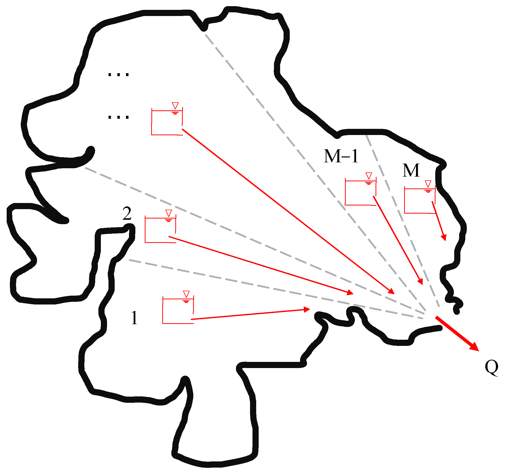
The rainfall–runoff simulation approximates the watershed as a time-invariant linear hydrological system. The simulation assumes that the regulation and storage of the watershed’s net rain on the surface can be represented by the regulation of M parallel linear reservoirs, as illustrated in Figure 2. Each linear reservoir within the confluence adheres to the watershed’s water storage equation and the conservation law of mass [28]. The unit hydrograph is divided into three sections. The rising and recessing sections follow the “exponential” pattern of growth and decline. As time approaches infinity, the unit hydrograph tends to zero [30]. The equation for the instantaneous unit hydrograph is obtained through the superposition of multiple negative exponential functions [29,31]. It can be expressed as

$$u_{(t)}=\frac{\mu }{t_p}{e}^{\frac{\mu }{t_p}(t-t_p)}{(1+m{e}^{\frac{\mu }{t_p}(t-t_p)})}^{-(1+1/m)}$$

(1)

where $u_{(t)}$ represents the instantaneous unit hydrograph; $\mu$ represents the rising coefficient determined by watershed characteristics (s); $t_p$ represents the time interval from the peak of net rainfall to the peak of flood (s); $m$ represents the recessing coefficient affected by the downstream water surface conditions.

To make $\mu$ dimensionless, we can perform a transformation by letting $\frac{\mu }{t_p}\to \mu$. This transformation leads to the general unit hydrograph $g_{\left(T\right)}$:

$$g_{(T)}={\displaystyle \underset{0}{\overset{T}{\int }}{u}_{(t)}}dt=1-{\left\{1+m{e}^{\left[\mu (T-t_p)\right]}\right\}}^{-1/m}$$

(2)

Given the knowledge of the surface runoff $R_{S(\mathrm{t})}$ for different durations $\Delta \tau$ (starting at $t=\tau$ and ending at $t=\tau +\Delta \tau$), the general unit hydrograph can be employed to deduce the corresponding surface runoff $Q_{s,t}$:

$$\begin{array}{ll}{Q}_{s,t}& ={\displaystyle \sum _{\tau }F\times R_{s(\tau )}}\frac{1}{\Delta \tau }[g_{\left(t-\tau \right)}-g_{(t-\tau -\Delta \tau )}]\\ & ={\displaystyle \sum _{\tau }F\times R_{S(\tau )}}\frac{1}{\Delta \tau }\left\{{\left[1+m{e}^{\mu (t-\tau -\Delta \tau -t_p)}\right]}^{-1/m}-{\left[1+m{e}^{\mu (t-\tau -t_p)}\right]}^{-1/m}\right\}\end{array}$$

(3)

where $Q_{s,t}$ represents the surface runoff at time t (m³·s⁻¹); F represents the watershed area (m²); $\Delta \tau$ represents rainfall duration starting at $t=\tau$ and ending at $t=\tau +\Delta \tau$; $R_{S(\tau )}$ represents the surface runoff depth in duration $\Delta \tau$ (m); $\tau$ represents a dummy variable in terms of time starting at $\tau =0$ and ending at $\tau =t$ (s). For the selected flood data, we assume that $\tau$ changes with a magnitude equal to the selected time step, which is 1 in this case.

2.3.2. SCE-UA Algorithm

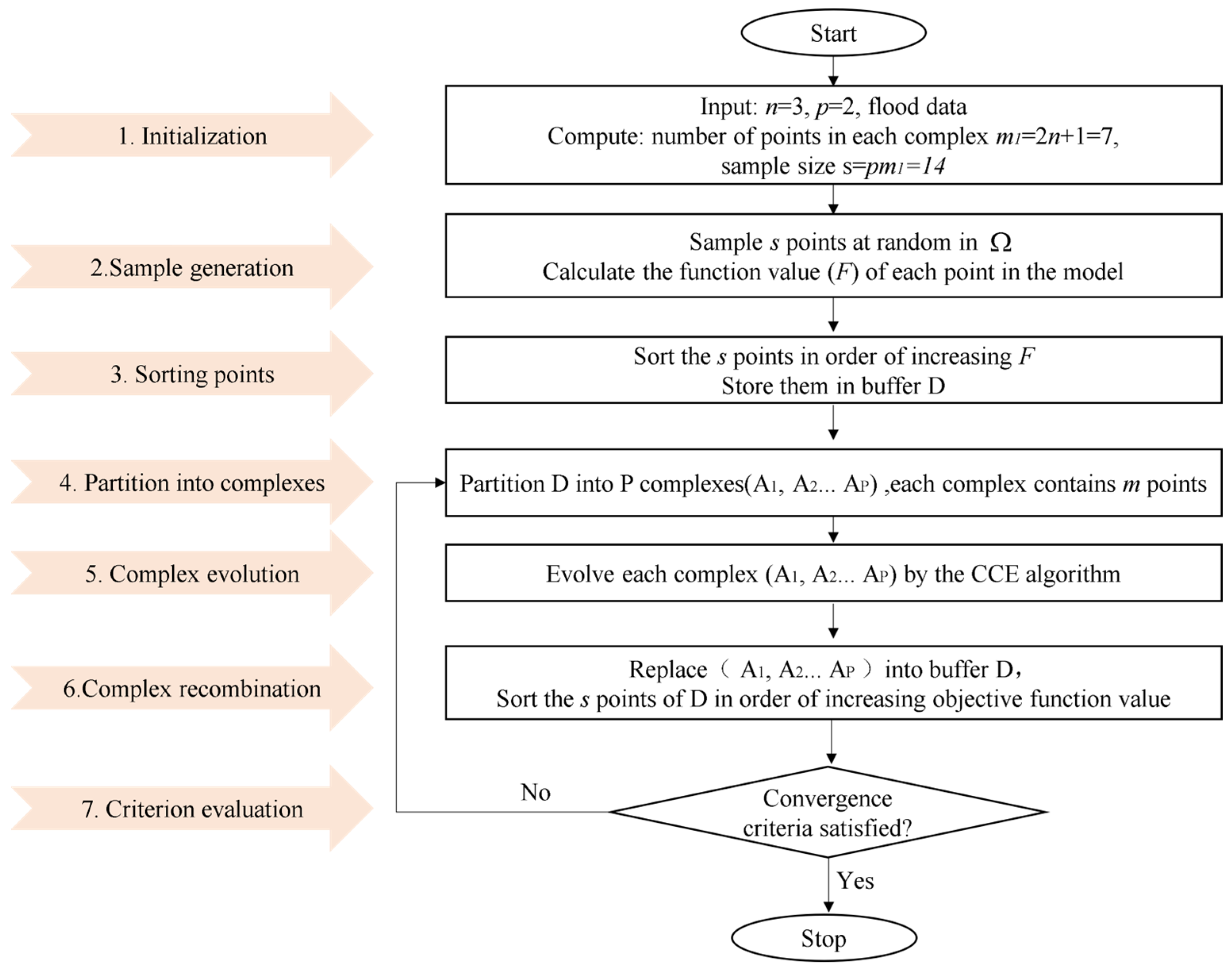
The SCE-UA algorithm is an efficient and robust global optimization method, known for its ability to effectively exploit population information, thereby enhancing algorithm convergence speed. The method integrates four key concepts: (1) a combination of deterministic and probabilistic approaches; (2) systematic evolution across point groups in the parameter space to achieve global improvement; (3) competitive evolution; (4) complex recombination [35]. Complex recombination improves survival capability by enabling the sharing of independently acquired information about the search space among the complexes. While the SCE-UA algorithm involves numerous parameters, most of them can adopt default values based on existing research findings. The determination of the complex number “p” is the only parameter, which needs to be tuned based on the specific problem at hand [40]. Based on the recommendation in the literature, “p” represents the number of complexes; “n” represents the number of parameters; “m₁” represents the number of vertices in each complex; “q” represents the number of vertices in each subcomplex; “s” represents the population size; while “α” and “β” correspond to the number and algebraic characteristics of offspring generated from the parent generation; the values of the parameters are defined as follows: m₁ = 2n + 1, q = n + 1, s = pm₁, α = 1, and β = 2n + 1 [35]. Figure 3 illustrates the flowchart framework of the SCE-UA method employed in this study. Here, we provide a detailed description of the method:

• Initialization: Set the dimensionality of the problem, “p” (value = 2); the value of “n” is 3 in the calculation process using the general unit hydrograph method, which involves only three parameters: $\mu$, $m$, $t_p$; “m₁” (value = 7); “s” (value = 14).
• Sample generation: Randomly generate s sample points within the feasible parameter space and compute the criterion value F for each point. F comprises four components: $f_{NSE}$ denotes the Nash efficiency coefficient function; $f_{R^2}$ represents the determination coefficient function; $f_{RE}$ corresponds to the absolute error function; and $f_{\Delta t}$ symbolizes the peak time difference function.

  $$F=0.6\times (f_{NSE}+f_{R^2})+0.2\times (1-f_{RE})+0.2\times (1-f_{\Delta t})$$

  (4)
• Sorting points: Arrange the s points in descending order based on their criterion values, with the first point corresponding to the maximum F value and the last point representing the F value (in the study, the maximum value is considered as the objective function).
• Partition into complexes: Divide the s points into p complexes, where each complex contains m points.
• Complex evolution: Evolve each complex using the competitive complex evolution (CCE) algorithm.
• Complex recombination: Merge the points from the evolved complexes into a sample population; sort this population in ascending order of F.
• Criterion evaluation: If the termination criteria are satisfied, stop; otherwise, go to Step 4. The convergence criteria for the optimization process are as follows: the iteration terminates when the objective function F attains the maximum allowable value or when the rate of change satisfies the specified minimum ratio (0.01%), indicating convergence.

2.3.3. SCE-GUH Model

This study investigates the suitability of the general unit hydrograph routing calculation for hydrological forecasting and flood disaster defense by analyzing the characteristics of its flow routing calculation. A relatively simple two-source model is implemented, where the routing module is divided into surface runoff and groundwater runoff components. The linear reservoir method, a well-established approach, is utilized to compute the groundwater runoff by simulating the processes of groundwater storage and release. To compute the surface runoff, the general unit hydrograph recession calculation, investigated in this study, is utilized, with parameter values being optimized using the SCE-UA algorithm. The SCE-GUH model integrates the SCE-UA optimization algorithm with the general unit hydrograph routing method. Specifically, the coupling process involves iterative computation. Initially, the SCE-UA algorithm generates a set of parameters for optimization, determined by the specified parameter range and initial values. Subsequently, these parameter values are utilized to compute the output of the general unit hydrograph method, which is compared with observed data in order to obtain the objective function, serving as an indicator for model fitting. Subsequently, the SCE-UA algorithm employs specific strategies to update or adjust the parameters, considering the current parameter values and the objective function. These changes may include parameter increases, decreases, or substitutions. The updated parameter values are subsequently employed to calculate the output of the general unit hydrograph routing method, repeating the process for the subsequent round of computing the statistic and adjusting the parameters. This process continues until the statistic achieves its maximum value or meets other specified stopping criteria. In summary, the aim of integrating the optimization algorithm with the model is to iteratively update the parameters and identify the parameter combination, which optimally aligns the general unit hydrograph routing method with real-world observed data, ultimately enhancing the SCE-GUH model’s applicability and predictive accuracy.

2.3.4. Model Benchmarks and Methods

Multiple benchmarks were employed to assess the performance of the SCE-GUH model. These benchmarks comprise Nash’s instantaneous unit hydrograph (NIUH), Nash’s instantaneous unit hydrograph coupled with the SCE-UA algorithm model (SCE-NIUH), and traditional general unit hydrograph (GUH). The model construction framework is depicted in Figure 4. The 53 flood scenarios employed for model calibration and verification are consistent, which is the premise for comparing the performance of different benchmarks. Among the four watersheds, we select flood events with strong data availability, where the first 70% of the data is used as the calibration period, and the remaining 30% is used as the validation period. Both the calibration and validation periods encompass different hydrological conditions, such as drought periods, normal periods, and high-flow periods, to ensure the model performs well under various hydrological conditions. We concurrently calculated and compared the performance evaluation metrics of all benchmarks.

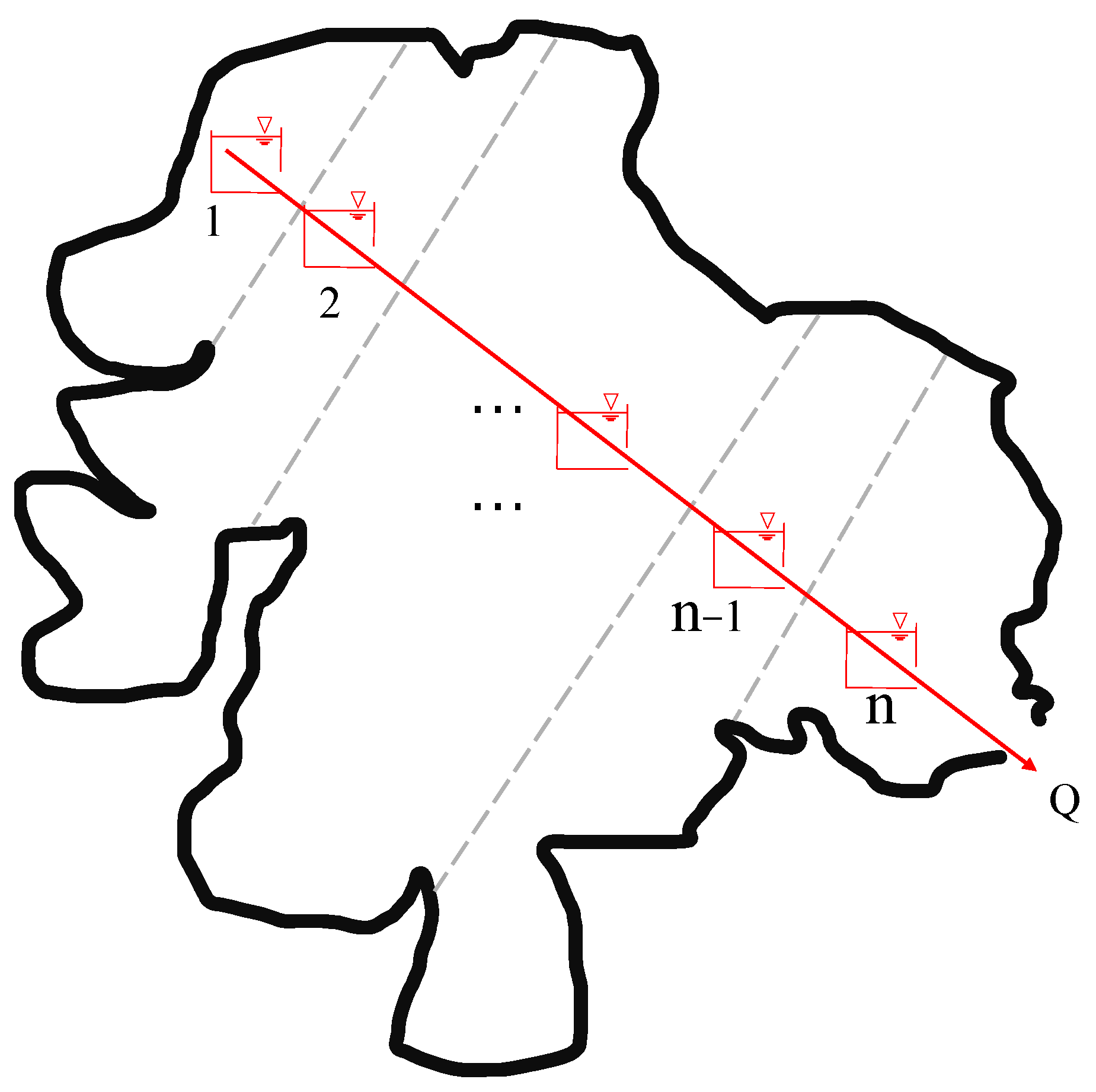
The NIUH and SCE-NIUH models were calculated using the Nash unit hydrograph method, which assumes linearity and time invariance in the watershed’s response, treating the watershed as a sequence of linear reservoirs connected in series, depicted in Figure 5. The Nash unit hydrograph calculates the confluence using the gamma function distribution, which has emerged as one of the most frequently utilized methods for confluence calculation [22,41].

2.3.5. Selection of Evaluation Indicators

The mathematical expressions for these metrics can be described as follows.

The average Nash–Sutcliffe efficiency coefficient (NSE) quantifies the model’s ability to predict variables deviating from the mean. It indicates the proportion of the initial variance explained by the model and varies from −∞ to 1, where 1 represents a perfect fit. Higher values closer to 1 indicate more accurate predictions:

$$NSE=1-\frac{{\displaystyle \sum _{i=1}^n{(Q_S^i-Q_O^i)}^2}}{{\displaystyle \sum _{i=1}^n{(Q_S^i-\overline{Q_O})}^2}}$$

(5)

where n represents the total number of measured data; $Q_S^i$ and $Q_O^i$ denote the simulated and observed discharge, respectively; ${\overline{Q}}_0$ represents the average observed discharge.

The coefficient of determination (R²) is commonly employed to quantify the level of fit between data. A higher R² value indicates a stronger association with the reference equation, while a lower R² value (closer to 0) implies a weaker association, as illustrated in Equation (5):

$$R^2=\frac{{\left[{\displaystyle {\sum }_{i=1}^n(Q_S^i-\overline{Q_S})(Q_O^i-\overline{Q_O})}\right]}^2}{{\displaystyle {\sum }_{i=1}^n{(Q_S^i-\overline{Q_S})}^2{(Q_O^i-\overline{Q_O})}^2}}$$

(6)

where ${\overline{Q}}_s$ represents the average simulated discharge.

The relative error (RE) is calculated by multiplying the ratio of the absolute error of a measurement to the actual value by 100%. Equation (6) shows the calculation. In the evaluation of flash flood models, RE is commonly employed to assess the reliability of the simulated flood peak discharge:

$$RE=\frac{Q_s^{\max }-Q_{\mathrm{o}}^{\max }}{Q_{\mathrm{o}}^{\max }}\times 100\%$$

(7)

where $Q_s^{\max },Q_{\mathrm{o}}^{\max }$ represent the maximum simulated peak discharge and observed peak discharge, respectively.

The absolute error of peak present time ($\Delta t$) can be calculated as the difference between the moment when the maximum flood discharge appears in the forecast process and the moment when it appears in the actual flood process. The formula to calculate $\Delta t$ is as follows:

$$\Delta t=t_s^{\max }-t_o^{\min }$$

(8)

where $t_s^{\max },t_o^{\min }$ represent the occurrence time of simulated and observed flood peaks, respectively.

3. Results

3.1. Model Calibration and Validation Results

The evaluation employs multiple discriminant indicators, including NSE, R², RE, and $\Delta t$. Considering the small drainage area and short flood duration in the study area, the allowable accuracy for predicting the flood peak is set at 20% of the measured flood peak. This implies that the predicted flood peak should be within ±20% of the actual observed value. Furthermore, a permissible deviation of up to 3 h is set for the peak time to avoid significant differences between the predicted and actual peak times.

Table 1. The parameter values were derived using the SCE-UA algorithm.

Watershed	SCE-GUH			SCE-NIUH
	m	tp/h	μ	n	k
Lixin	1.60	0.96	2.18	1.61	3.32
Xiagushan	1.90	0.60	0.20	1.86	3.74
Liqingdian	6.70	2.10	2.50	2.53	3.11
Miping	1.00	2.00	1.50	2.79	4.40

presents the optimal parameter values utilized in computing surface flow concentration using the SCE-UA algorithm. These parameters are determined during the calibration process of the SCE-GUH model and the SCE-NUIH model.

A total of 39 representative floods were selected from 53 flood events in four watersheds: 12 from the Lixin watershed, 11 from the Xiagushan watershed, 8 from the Liqingdian watershed, and 8 from the Miping watershed. The selection process aimed to capture a range of different flood characteristics. The simulation results of the four models during the parameter calibration period are presented in

Table 2. Summary table of simulated results for flood events during the calibration period.

Basin	RE/%				Nse				R2				△t/h
	NUIH	SCE-NUIH	GUH	SCE-GUH	NUIH	SCE-NUIH	GUH	SCE-GUH	NUIH	SCE-NUIH	GUH	SCE-GUH	NUIH	SCE-NUIH	GUH	SCE-GUH
Lixin	14.21	17.30	9.70	11.35	0.69	0.73	0.75	0.82	0.73	0.74	0.79	0.85	0.67	0.50	0.42	0.17
Xiagushan	14.33	15.72	8.55	8.40	0.73	0.76	0.80	0.82	0.75	0.83	0.84	0.85	0.82	1.00	0.73	0.45
Liqingdian	12.13	12.52	13.35	12.60	0.71	0.76	0.82	0.84	0.79	0.86	0.87	0.87	1.13	1.00	0.75	0.75
Miping	13.70	16.78	8.21	5.54	0.70	0.72	0.83	0.87	0.75	0.79	0.93	0.95	2.38	2.38	0.63	0.63

, and Figure 6 illustrates the simulated hydrograph. The hydrographs generated by the NIUH, SCE-NIUH, GUH, and SCE-GUH models exhibit a close agreement with the observed hydrographs. These representative floods were utilized for model parameter calibration.

We conducted 12 typical flood simulations in the Lixin watershed. The average RE calculated for these simulations were 14.21%, 17.30%, 9.70%, and 11.35% for the NIUH, SCE-NIUH, GUH, and SCE-GUH models, respectively. The respective models achieved peak flow rates with qualification rates of 83.33%, 83.33%, 100%, and 100%. $\Delta t$ across all four models were determined as 0.67 h, 0.50 h, 0.42 h, and 0.17 h, respectively. Each model achieved a peak flow time qualification rate of 100%. The average NSE values for the NIUH, SCE-NIUH, GUH, and SCE-GUH models were 0.69, 0.73, 0.75, and 0.82, respectively. Additionally, the corresponding R² values were 0.73, 0.74, 0.79, and 0.85. However, when performing calculations with the NIUH model, the relative errors of peak flow rates for the floods on 14 June 1984 and 20 July 1987 exceeded 20%, violating the allowable error threshold. In contrast, the flood simulations conducted using the GUH model produced peak flow rates, which closely matched the measured flow rates within the acceptable error limit for both floods. It is worth noting that the simulation results obtained from the GUH model exhibited superior performance compared to the NIUH model in terms of RE, peak flow rate qualification, R², $\Delta t$, and NSE. We simulated 11 typical flood events in the Xiagushan watershed using four models: NIUH, SCE-NIUH, GUH, and SCE-GUH. The RE of the average simulation results for these models were obtained and found to be 14.33%, 15.72%, 8.55%, and 8.40%, respectively. The flood peak qualification rates for each model were calculated as 90.91%, 90.91%, 100%, and 100%, respectively. The $\Delta t$ were 0.82 h, 1 h, 0.73 h, and 0.45 h, respectively. Furthermore, all four models achieved a peak timing qualification rate of 100%. Moreover, the average NSE values were 0.73, 0.76, 0.80, and 0.82, and the average R² values were 0.75, 0.83, 0.84, and 0.85, respectively. It is worth noting that applying the SCE-NIUH model in this watershed resulted in an overall improvement of 0.03 in NSE and 0.08 in R² compared to the NIUH model. However, the simulations of average RE and $\Delta t$ using the SCE-NIUH model slightly underperformed compared to the NIUH model. This discrepancy can be attributed to the SCE-UA algorithm, which assigns an NSE proportion of up to 0.6 during parameter calibration for the objective function and prioritizes improving the model’s NSE [42]. Additionally, the simulation results using GUH for flow routing showed significant improvements over the NIUH. Moreover, the simulation results using the SCE-GUH model outperformed the GUH model. Specifically, the average RE and $\Delta t$ values were reduced by 0.15% and 0.28 h, respectively, and the average NSE and R² improved by 0.02 and 0.01, respectively, compared to the GUH model.

We simulated eight typical flood events in the Liqingdian watershed using four models: NIUH, SCE-NIUH, GUH, and SCE-GUH. The resulting average RE values for the models were 12.13%, 12.52%, 13.35%, and 12.60%, respectively. While the RE values of other models decreased compared to the NIUH model, all models (except NIUH, with a peak flow rate passing the rate of 87.5%) achieved a 100% pass rate. The average $\Delta t$ were obtained as 1.13 h, 1 h, 0.75 h, and 0.75 h, corresponding to peak time pass rates of 87.50%, 90.91%, 100%, and 100%, respectively. Moreover, the NIUH, SCE-NIUH, GUH, and SCE-GUH models achieved average NSE values of 0.71, 0.76, 0.82, and 0.84, and average R² values of 0.79, 0.86, 0.87, and 0.87, respectively. A case analysis of the flood event, which occurred on 23 July 2005, showed that the NUIH model had RE, $\Delta t$, and NSE values of 15.38%, 5 h, and 0.71, respectively, while for the SCE-NIUH model, the corresponding values were 16.7%, 4 h, and 0.71, respectively. In contrast, the GUH model produced RE, $\Delta t$, and NSE values of 13.36%, 1 h, and 0.79, and the SCE-GUH model had values of 13.38%, 1 h, and 0.78, respectively. It is important to note that utilizing the NIUH model led to a $\Delta t$ value for the flood event, which exceeded the acceptable error range. While the SCE-UA algorithm reduced the error by 1 h, it still exceeded the forecast accuracy standards. However, by utilizing the GUH model, enhancements in NSE were observed, and $\Delta t$ was significantly reduced to 1 h, effectively controlling it within the allowable error range.

We conducted eight typical flood simulations in the Miping watershed using four models, namely NIUH, SCE-NIUH, GUH, and SCE-GUH. The average RE values for these models were determined as 13.70%, 16.78%, 8.21%, and 5.54%, respectively. The qualification rates for flood peak accuracy were recorded as 87.50%, 87.50%, 100%, and 100% for these models, respectively. The average $\Delta t$ values were determined as 2.38 h, 2.38 h, 0.63 h, and 0.63 h for the four models, respectively, while achieving qualification rates of 75%, 75%, 100%, and 100%. The average NSE values were calculated as 0.70, 0.72, 0.83, and 0.87 for the NIUH, SCE-NIUH, GUH, and SCE-GUH models, respectively. The average R² values were 0.75, 0.79, 0.93, and 0.95 for NIUH, SCE-NIUH, GUH, and SCE-GUH, respectively. Notably, the NIUH and SCE-NIUH models displayed significant errors in simulating the floods, which occurred on 4 September 2003 and 1 October 2005, with average $\Delta t$ of 4 h and 6 h, respectively. In contrast, the GUH and SCE-GUH models precisely reproduced the timing of flood peaks observed in the actual hydrographs. Consequently, there was a significant improvement in the NSE values, with the NIUH model transitioning from 0.67 and 0.62 to 0.75 and 0.73, and the SCE-NIUH model transitioning from 0.67 and 0.65 to 0.80 and 0.81 for the GUH and SCE-GUH models, respectively.

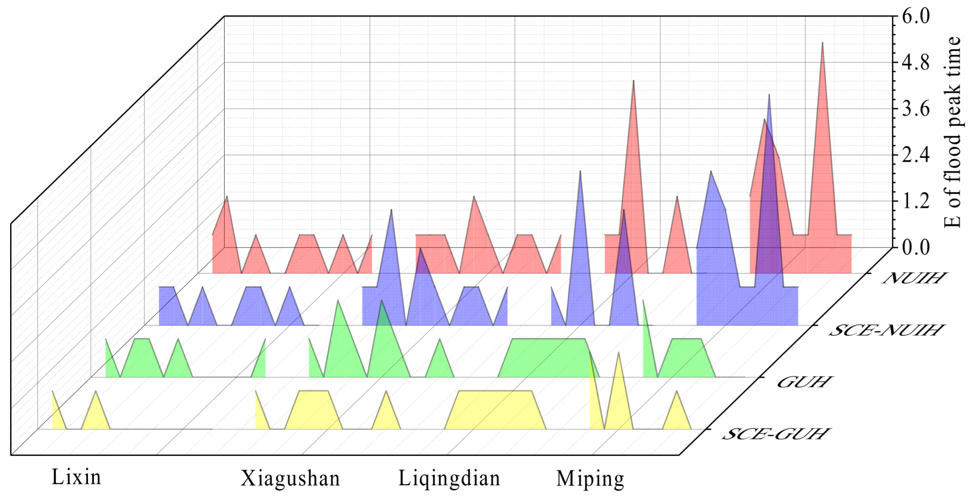
The simulation results of the four models, based on the application practices during the calibration period in four watersheds, demonstrate that the general unit hydrograph algorithm significantly outperforms the NIUH algorithm in terms of controlling peak timing error and relative peak flow error. Figure 7 illustrates the error in peak present time. Additionally, calibrating unit hydrograph parameters using the SCE-UA algorithm can enhance simulation accuracy. This demonstrates that the optimized parameter values are reasonably close to the true values, making them suitable for broader application. In summary, the performance of the four models can be ranked as follows: SCE-GUH > GUH > SCE-NIUH > NIUH.

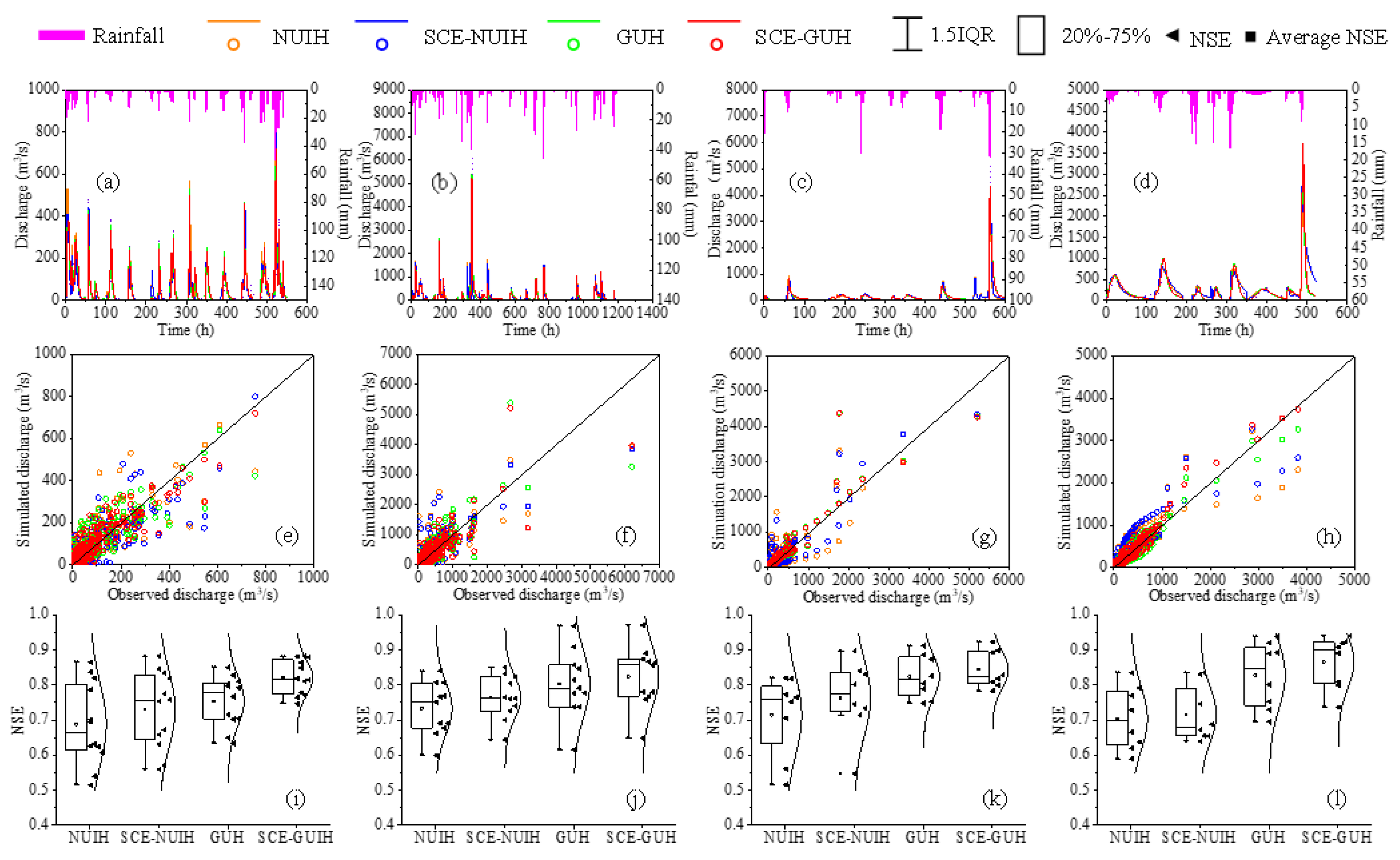
The verification period involved four typical flood events in the Lixin and Xiagushan watersheds, respectively, as well as three events in the Liqingdian and Miping watersheds, respectively.

Table 3. Table of simulated results during the validation period for flood events. In the relative error, a negative sign (−) indicates that the simulated peak flow is lower than the observed flow. In the peak timing error, a negative sign (−) indicates that the simulated peak occurs earlier than the actual peak.

Number	RE/%				Nse				R2				△t/h
	NUIH	SCE-NUIH	GUH	SCE-GUH	NUIH	SCE-NUIH	GUH	SCE-GUH	NUIH	SCE-NUIH	GUH	SCE-GUH	NUIH	SCE-NUIH	GUH	SCE-GUH
Lixin watershed
20030830	−2.22	−15.76	−5.83	1.19	0.89	0.93	0.92	0.94	0.93	0.95	0.95	0.96	0	0	0	0
20050708	10.47	13.33	8.19	11.42	0.79	0.94	0.82	0.87	0.84	0.88	0.88	0.90	0	0	0	0
20080722	10.39	−15.23	−12.23	−5.54	0.54	0.72	0.77	0.83	0.70	0.77	0.82	0.85	−1	−1	−1	−1
2010019	7.71	−14.30	−16.21	−16.14	0.73	0.78	0.81	0.86	0.81	0.85	0.88	0.89	0	0	0	0
Average	7.70	14.66	10.62	8.57	0.73	0.82	0.83	0.87	0.82	0.86	0.88	0.90	0.25	0.25	0.25	0.25
Xiagushan watershed
20000714	−85.90	−57.85	−25.88	−18.66	0.52	0.61	0.59	0.60	0.62	0.65	0.62	0.63	0	0	−1	1
20020626	−4.30	−16.26	0.20	6.99	0.62	0.78	0.91	0.95	0.65	0.79	0.92	0.96	−1	−1	0	0
20100718	−0.84	−17.95	−7.24	−11.38	0.66	0.67	0.89	0.91	0.70	0.69	0.89	0.92	0	0	0	0
20130525	−1.62	3.50	1.87	5.53	0.71	0.79	0.86	0.89	0.72	0.79	0.86	0.89	3	3	0	0
Average	23.17	23.89	8.80	10.64	0.63	0.71	0.81	0.84	0.67	0.73	0.82	0.85	1	1	−0.25	0.25
Liqingdian watershed
20100819	−23.99	−17.58	0.77	1.28	0.62	0.59	0.72	0.73	0.72	0.63	0.76	0.76	1	1	−1	1
20100823	4.46	10.23	3.95	6.23	0.70	0.76	0.77	0.81	0.79	0.85	0.82	0.84	3	0	−3	3
20110914	1.02	8.92	−8.55	−3.35	0.80	0.88	0.93	0.94	0.88	0.94	0.95	0.95	0	1	0	0
Average	9.82	12.24	4.42	3.62	0.71	0.74	0.80	0.83	0.8	0.81	0.84	0.85	1.33	0.67	1.33	1.33
Miping watershed
20090816	−17.62	−19.04	−12.74	−7.06	0.54	0.55	0.86	0.85	0.73	0.75	0.86	0.87	3	1	−1	−1
20100724	−7.81	−2.60	−7.69	−4.86	0.79	0.83	0.88	0.88	0.89	0.89	0.89	0.89	−1	−1	2	2
20110913	0.81	4.62	−3.13	1.59	0.75	0.82	0.92	0.91	0.84	0.87	0.93	0.93	1	1	1	−1
Average	8.75	8.75	7.85	4.50	0.69	0.73	0.89	0.88	0.82	0.84	0.89	0.90	1.67	1	1.33	1.33

provides the simulated results for flood events during the verification period, whereas Figure 8 illustrates the simulated rainfall and runoff, along with the performance evaluation chart of the four models throughout this period.

The four models in the Lixin watershed all achieved a total qualification rate of 100%. There was a 1 h time lag for the flood event, which occurred on 22 July 2008, while no time lag was observed for other events. The average NSE values for the four models, namely NIUH, SCE-NIUH, GUH, and SCE-GUH, were 0.73, 0.82, 0.83, 0.87, while the average R² values were 0.82, 0.86, 0.88, 0.90, respectively. In the Xiagushan watershed, the RE values for simulating the typical flood event on 14 July 2000 were 85.90%, 57.85%, 25.88%, and 18.66% for the NIUH, SCE-NIUH, GUH, and SCE-GUH models, respectively. The total qualification rates for the NUIH, SCE-NUIH, GUH, SCE-GUH models were 75%, 75%, 75%, and 100%, respectively, with average time lags of 1 h for the NIUH and SCE-NIUH models, and 0.25 h for the GUH and SCE-GUH models. The average NSE values for the models were 0.63, 0.71, 0.81, and 0.84, while the average R² values were 0.67, 0.73, 0.82, and 0.85, respectively. In the Liqingdian watershed, the RE values for the four models during the flood event on 19 August 2010 were 23.99%, 17.58%, 0.77%, and 1.28% for NUIH, SCE-NUIH, GUH, and SCE-GUH, respectively. Consequently, the NUIH model had a total qualification rate of only 66.67%. However, the simulation results of the other three models were within the acceptable prediction error range, resulting in a total qualification rate of 100%. The SCE-NIUH model had an average time lag of 0.67 h, while the other three models had an average time lag of 1.33 h. The average NSE values for the models were 0.71, 0.74, 0.80, 0.83, respectively. Similarly, the average R² values were 0.80, 0.81, 0.84, and 0.85, respectively. The four simulated models in the Miping watershed all achieved a total qualification rate of 100%. The average time lags for the NUIH, SCE-NUIH, GUH, SCE-GUH models were 1.67 h, 1 h, 1.33 h, and 1.33 h, respectively. The average NSE values for the models were 0.69, 0.73, 0.89, and 0.88, while the average R² values were 0.82, 0.84, 0.89, and 0.90, respectively. Figure 9 shows the errors in peak time presentation for the four watersheds based on the four methods.

We conducted a comprehensive performance analysis of the four models across the selected watersheds. The SCE-GUH model was calibrated, and the average values of NSE, R², RE were found to be 0.82, 0.85, 11.35%, respectively, with $\Delta t$ of 1.67 h in the Lixin watershed. The calibration period yielded results of 0.82 for NSE, 0.85 for R², 8.40% for RE, and $\Delta t$ of 0.45 h in the Xiagushan watershed. Average values of 0.84 (NSE), 0.87 (R²), 12.60% (RE), and 0.75 h ($\Delta t$) were obtained in the Liqingdian watershed. The values during the calibration period were 0.87 for NSE, 0.95 for R², 5.54% for RE, and $\Delta t$ of 0.63 h in the Miping watershed. The SCE-GUH model was validated, and the average values of NSE, R², RE were found to be 0.87, 0.90, 8.57%, respectively, with $\Delta t$ of 0.25 h in the Lixin watershed. The validation period yielded results of 0.84 for NSE, 0.85 for R², 10.64% for RE, and $\Delta t$ of 0.25 h in the Xiagushan watershed. Average values of 0.83 (NSE), 0.85 (R²), 3.62% (RE), and 1.33 h ($\Delta t$) were obtained in the Liqingdian watershed. The values during the validation period were 0.88 for NSE, 0.90 for R², 4.50% for RE, and $\Delta t$ of 1.33 h in the Miping watershed. Thus, it can be concluded that the SCE-GUH model demonstrates favorable applicability in simulating rainfall and runoff in the four watersheds.

The peak occurrence time errors for Lixin, Xiagushan, Liqingdian, and Miping in the SCE-GUH model were 0.19 h, 0.40 h, 0.91 h, and 0.82 h, respectively. In the GUH model, the errors were 0.38 h, 0.60 h, 0.91 h, 0.82 h. In the SCE-NUIH model, the errors were 0.38 h, 1.00 h, 0.91 h, 2.00 h. In the NUIH model, the errors were 0.51 h, 0.87 h, 1.18 h, 2.19 h. Compared with the other three models, the SCE-GUH model showed a significant reduction in peak time error. Among the four studied watersheds, the peak time qualified rate was 100% in both the GUH and SCE-GUH models, while in the NUIH and SCE-NUIH models, the qualified rates were only 81.80% in the Miping watershed and 90.91% in the Liqingdian watershed. The NSE values for the four watersheds in the SCE-GUH model were 0.83, 0.83, 0.84, 0.87; in the GUH model, the values were 0.77, 0.81, 0.82, 0.84; in the SCE-NUIH model, the values were 0.75, 0.75, 0.76, 0.72; in the NUIH model, the values were 0.70, 0.70, 0.71, 0.70. By comparing the results, it can be observed that the SCE-GUH model improved the fitting degree of the flood hydrograph. Analyzing the overall qualification rate of the four watersheds, the SCE-GUH model achieved a 100% qualification rate. The GUH model had the second highest qualification rate, with all watersheds except Xiagushan achieving a 100% qualification rate. It is worth noting that the overall qualification rate of the Xiagushan watershed is 93.33%. However, in the SCE-NUIH model, only the Liqingdian watershed achieved a 100% qualification rate, while the other three watersheds had qualification rates of 87.5% for Lixin, 86.67% for Xiagushan, and 72.73% for Miping. In the NUIH model, the highest qualification rate was 87.50% in the Lixin watershed, while the lowest qualification rate was only 72.73% in the Liqingdian and Miping watersheds. Fluctuations occurred between the observed and simulated data during the simulation process of the four models. The main reasons for these fluctuations can be summarized as follows. First, there is an error in calculating the runoff phase. Second, in some cases, the rainfall during flood events exhibits scattered patterns, characterized by multiple rainfall peaks and downstream accumulation. The centralized model employed in this experiment utilized Thiessen polygons for processing rainfall, but it neglected the uneven spatial distribution of rainfall, leading to an error in simulating the flow rate. Lastly, the time intervals for the measured flow data are inconsistent. The study utilized a 1 h interval obtained through interpolation, which might compromise the accuracy of the simulation results.

The comparison among the four models reveals that the model constructed with the general unit hydrograph produces superior simulation results in comparison to the model, which uses the same conditions but relies on the Nash unit hydrograph. Consequently, the general unit hydrograph model, by utilizing runoff calculations, provides a more accurate depiction of the hydrological processes within the watershed compared to the Nash unit hydrograph model. This finding significantly contributes to enhancing our understanding and facilitating efficient management of water resources within the watershed.

3.2. Typical Site Flood Analysis

Figure 10a presents the simulation results of the flood event of 4 August 1995 in the Lixin watershed using four models, NIUH, SCE-NIUH, GUH, and SCE-NIUH, with corresponding $\Delta t$ of 1 h, 1 h, 0, and 0. The NSE values for these models were 0.62, 0.63, 0.79, and 0.88, respectively. The comparison clearly shows that applying the general unit hydrograph method significantly enhances the accuracy of flood forecasting and reduces errors in predicting the timing of peak flow. Furthermore, optimizing the parameters of the SCE-UA algorithm led to additional enhancements in the NSE. The floods, which occurred on 20 August 1995, were studied in the Xiagushan watershed. The RE for this flood, as predicted by the four models, were 12.79%, 3.90%, 5.90%, and 0.61%. The $\Delta t$ used in the models were 1 h, 1 h, 0, and 0, while the NSE values were 0.81, 0.82, 0.97, and 0.97, correspondingly. Figure 10b demonstrates that the rising and falling water process, specifically in the rising and falling water section, based on the GUH model closely resembles the observed process. The peak time is in perfect agreement with the measured process. In contrast, the total duration of the confluence as predicted by the NIUH differs from the observed process and is considerably shorter in duration. The results indicate that the SCE-GUH model demonstrates superior simulation performance. Moreover, the application of the general unit hydrograph method significantly enhanced the accuracy of flood forecasting while reducing the discrepancy between the simulated time of peak occurrence and the actual observed time of peak occurrence. By optimizing the parameters of the SCE-UA algorithm, the NSE and the rate of prediction qualification were further improved to a certain extent. The simulation of the flood event, which occurred on 14 September 2011 in the Liqingdian watershed, indicates that the RE and $\Delta t$ values obtained from the four models fall within an acceptable range. Moreover, the NSE values exceed 0.80, indicating satisfactory simulation results. Please refer to Figure 10c for the simulation hydrograph. The simulation results of the four models exhibit a high degree of similarity during the rising stage of the flood. However, during the initial phase of recession, the two models based on NIUH and SCE-NIUH demonstrate a noticeably slower decline in the simulated flood compared to the observed flood. Nevertheless, the parameter $m$ utilized in the calculations for both the GUH and SCE-GUH models partly accounts for the regression rate by incorporating the hydrological characteristics of the watershed. This integration helps align the simulated regression process more closely with the observed regression process. Figure 10d presents the simulation results of the flood event, which occurred on 29 July 2007 in the Miping watershed, using four models: NIUH, SCE-NIUH, GUH, and SCE-NIUH. The RE for these models were 19.00%, 16.82%, 17.01%, and 2.20%, respectively. The $\Delta t$ were 1 h, 1 h, 0, and 0, respectively. Additionally, the NSE values were 0.64, 0.69, 0.94, and 0.94, respectively. The simulation results for the rising and falling stages of this flood exhibit considerably higher accuracy in the GUH and SCE-GUH models compared to the NUIH and SCE-NUIH models. This flood is categorized as a major flood; due to the NUIH and SCE-NUIH models’ sensitivity to early rainfall, within the first 10 h of rainfall, the water levels rise rapidly, and the flood peak recedes swiftly after reaching its maximum. These processes occur at a shorter duration compared to the observed measurements. Moreover, the flood peak emerges earlier than recorded in the observation period. This suggests that the SCE-GUH model exhibits superior simulation performance, followed by the GUH model in the second place. Conversely, the SCE-NUIH and NUIH models perform notably worse than the previously mentioned two models in simulating this flood event.

The combined use of the general unit hydrograph and the SCE-UA algorithm holds significant practical implications. The ranking order of flood simulation performance for the four models in the four watersheds is as follows: SCE-GUH > GUH > SCE-NIUH > NIUH. The concentration calculation equation of the general unit hydrograph is based on a negative exponential function, according to the calculation principle. The parameters, such as $\mu$ and $m$, partially reflect the watershed characteristics and control the amplitude of flood rise and fall [31]. The convergence of the Nash unit hydrograph is typically calculated using a gamma function with parameter n. When calculating runoff from the instantaneous unit hydrograph S curve, a table lookup is commonly used [43]. Consequently, the general unit hydrograph convergence model exhibits higher flexibility and is more aligned with the actual confluence process. The Nash unit hydrograph is based on the fundamental assumption of a linear reservoir series within the watershed [17]. Higher sensitivity to net rainfall is observed when the current soil moisture content is relatively high, resulting in a greater change in the hydrograph amplitude compared to the measured hydrograph. The three parameters of the general unit hydrograph integrate rainfall characteristics and watershed features, including water system shape and watershed slope, based on the analysis of parameter characteristics [28]. For instance, in the case of the Liqingdian watershed, which possesses a parallel water system with an elevation difference close to 2000 m, incorporating these factors into the confluence calculation leads to improved simulation results for rainfall–runoff. In conclusion, the application of the general unit hydrograph principle in the simulation of rainfall–runoff provides a more accurate characterization of watershed catchment characteristics compared to the Nash unit hydrograph.

3.3. Analysis of the Influence of Parameters on Unit Hydrograph

Extensive research had been conducted on the influence of Nash unit hydrograph parameters in the existing literature. Previous studies have revealed that two parameters in the Nash unit hydrograph exert a certain influence on the three elements of the unit hydrograph, namely peak flow, peak lag time, and total duration [20,44]. Nonetheless, further discussion is needed regarding the influence of the three parameters of the general unit hydrograph on the three elements of the unit hydrograph [28]. For instance, as an illustration, a net rainfall input of 10 mm per unit time period (1 h) in the Liqingdian watershed was considered. In the experiment, only one parameter was debugged at a time, allowing for an analysis of the effects of parameter changes on the three elements of the unit hydrograph. The results are depicted in Figure 11.

Figure 11a illustrates that as $\mu$ increases, the unit hydrograph exhibits a “tall and thin” shape, resulting in an increase in the flood peak, a decrease in the delay time of the flood peak, and a reduction in the total duration. The results presented in Figure 11b demonstrate that increasing the value of $m$ leads to a “squat” shape of the unit hydrograph, which in turn causes a decrease in the flood peak. However, the change in $m$ has minimal impact on the delay time and total duration of the flood peak. It is worth noting that at the end of the confluence, the flow will increase alongside the increase in m. The observation depicted in Figure 11c indicates that an increase in $t_p$ results in a “plump and flat” shape of the unit hydrograph. This change leads to a decrease in the flood peak, a significant increase in the delay time of the flood peak, and a significant extension of the total duration.

4. Discussion

The performance of the four constructed test models in the watershed is satisfactory. These models effectively capture the variations and attenuation of flood events, maintaining the simulation errors of peak flow and peak time within acceptable limits. Nevertheless, all models typically underestimate the magnitude of flood peaks, a common observation in other lumped models [6]. The performance of the four models is ranked as follows: SCE-GUH > GUH > SCE-NIUH > NIUH. This ranking result aligns with the expectations and validates the applicability of the SCE-GUH model, which outperforms the other three models in simulating episodic floods. The GUH model exhibited slightly better overall error control and simulations of flood fluctuation and dissipation compared to the NIUH model. Consistent with previous studies, this article’s research confirms that the general unit hydrograph method is more applicable than the Nash unit hydrograph method [29,30]. Furthermore, the SCE-GUH model exhibited superior overall performance compared to the GUH model. This is due to the effective reduction in errors in predicting peak flow and flood volume achieved by utilizing the complex evolutionary theory within the SCE-UA algorithm for parameter optimization. The model is also automatically calibrated to improve the NSE and R² based on the constraints of the objective function [38,42]. The SCE-GUH model demonstrates superior compliance in terms of the relative error of peak flow and enhances the correlation coefficient compared to other lumped models [45]. Overall, the SCE-GUH model demonstrates superior performance, notably in accurately simulating the peak flow and improving the correlation coefficient. This distinction sets it apart from other models in the field, making it a valuable tool for hydrological and flood prediction research. Regrettably, we did not consider the problem of target function divergence during the model construction process [46]. Further discussion is required to address the divergence issue, enhance convergence speed, and ensure the target function achieves the desired effect. Our experiments were conducted exclusively in small watershed areas, which are susceptible to flash floods in the Yangtze River and Huaihe River regions of China. The performance of this model may be influenced by variations in climate change, terrain, hydrological processes, and data availability across different regions. Consequently, further research is necessary to investigate the model’s applicability in other regions worldwide based on this theory, as well as to explore its practical utilization in decision support and disaster management.

5. Conclusions

This study introduces a new flood forecasting model, SCE-GUH, which combines the general unit hydrograph with the SCE-UA optimization algorithm. The SCE-GUH model is founded on a robust theoretical basis and substantiated by scientific evidence. The applicability of SCE-GUH in simulating flash flood was examined using data from 53 observed flash flood events in the Lixin, Xiagushan, Liqingdian, and Miping watersheds. Moreover, a comparison was made between the simulation results of SCE-GUH and those of the NIUH, SCE-NIUH, and traditional GUH models. The key findings of this study are summarized as follows.

The performance ranking of these four models across the four watersheds is as follows: SCE-GUH > GUH > SCE-NIUH > NIUH. The SCE-GUH model exhibits stability and robustness across various flood scenarios. The model’s structure is succinct, optimizing a mere three parameters. This reduces the risk of overfitting, lowers computational and storage costs, and enhances overall efficiency. The calculation formula of the general unit hydrograph method is relatively simple. The application of the general unit hydrograph enhances the description of surface runoff processes and introduces a new perspective into flood prediction research. Additionally, the application of the negative exponential function in the confluence is simpler compared to the gamma function (Nash unit hydrograph). This simplification reduces error transmission and the cumulative effect. The parameters involved in the calculation include the topographic and geomorphic characteristics of the watershed and the rainfall characteristics. Changes in these parameters have a significant impact on the three elements of the general unit hydrograph, with the flood peak being the most sensitive. The utilization of the SCE-UA composite optimization strategy for parameter optimization allows for an improved characterization of the catchment characteristics in the watershed, resulting in enhanced timeliness and prediction accuracy. Therefore, the SCE-UA model is well suited for regions prone to flash floods, where data are limited. By considering factors such as rainfall, soil moisture content, and topography comprehensively, it enables precise simulation of water flow and accumulation processes in a watershed, thus facilitating accurate prediction of flood propagation and evolution trends. Furthermore, this serves as a vital scientific basis for flood forecasting and prevention within the watershed while also providing a fresh perspective on international flash flood early warning and prediction. However, it is important to note that this experiment was only conducted in four selected flow domains, and its applicability should be tested further in other watersheds.

References

1. Zhang, Z. Characteristics of flash floods in China and their prevention and control ideas. China Water Resour. 2007, 14, 14–15. [Google Scholar]
2. Liu, C.; Guo, L.; Ye, L.; Zhang, S.; Zhao, Y.; Song, T. A review of advances in China’s flash flood early-warning system. Nat. Hazards 2018, 92, 619–634. [Google Scholar] [CrossRef] [Green Version]
3. Tamm, O.; Saaremäe, E.; Rahkema, K.; Jaagus, J.; Tamm, T. The intensification of short-duration rainfall extremes due to climate change—Need for a frequent update of intensity–duration–frequency curves. Clim. Serv. 2023, 30, 100349. [Google Scholar] [CrossRef]
4. Li, B.; Liang, Z.; Fu, Y.; Wang, J.; Hu, Y. A model for production and sink flow based on variable saturation zone and its parameter determination method. Adv. Water Sci. 2022, 33, 208–218. [Google Scholar]
5. Corral, C.; Berenguer, M.; Sempere-Torres, D.; Poletti, L.; Silvestro, F.; Rebora, N. Comparison of two early warning systems for regional flash flood hazard forecasting. J. Hydrol. 2019, 572, 603–619. [Google Scholar] [CrossRef] [Green Version]
6. Usman, M.; Ndehedehe, C.E.; Farah, H.; Ahmad, B.; Wong, Y.; Adeyeri, O.E. Application of a Conceptual Hydrological Model for Streamflow Prediction Using Multi-Source Precipitation Products in a Semi-Arid River Basin. Water 2022, 14, 1260. [Google Scholar] [CrossRef]
7. Georgakakos, K.P. Analytical results for operational flash flood guidance. J. Hydrol. 2006, 317, 81–103. [Google Scholar] [CrossRef]
8. Ntelekos, A.A.; Georgakakos, K.P.; Krajewski, W.F. On the uncertainties of flash flood guidance: Toward probabilistic forecasting of flash floods. J. Hydrometeorol. 2006, 7, 896–915. [Google Scholar] [CrossRef]
9. Tamm, O.; Kokkonen, T.; Warsta, L.; Dubovik, M.; Koivusalo, H. Modelling urban stormwater management changes using SWMM and convection-permitting climate simulations in cold areas. J. Hydrol. 2023, 622, 129656. [Google Scholar] [CrossRef]
10. He, B. Overview of flash flood warning methods of the Japan Meteorological Agency. China Flood Control Drought Relief 2020, 30, 149–152. [Google Scholar]
11. Bartholmes, J.C.; Thielen, J.; Ramos, M.H.; Gentilini, S. The european flood alert system EFAS—Part 2: Statistical skill assessment of probabilistic and deterministic operational forecasts. Hydrol. Earth Syst. Sci. 2009, 13, 141–153. [Google Scholar] [CrossRef] [Green Version]
12. Thielen, J.; Bartholmes, J.; Ramos, M.H.; de Roo, A. The European Flood Alert System—Part 1: Concept and development. Hydrol. Earth Syst. Sci. 2009, 13, 125–140. [Google Scholar] [CrossRef] [Green Version]
13. Cheng, W. A review of critical rainfall research on flash floods. Adv. Water Sci. 2013, 24, 901–908. [Google Scholar]
14. Guo, L.; Tang, X.; Kong, F. Research and application of flash flood early warning and forecasting system based on distributed hydrological model. China Water Resour. 2007, 14, 38–41. [Google Scholar]
15. Liu, Z.; Martina, M.L.; Todini, E. Flood forecasting using a fully distributed model: Application of the TOPKAPI model to the Upper Xixian catchment. Hydrol. Earth Syst. Sci. 2005, 9, 347–364. [Google Scholar] [CrossRef] [Green Version]
16. Koren, V.; Reed, S.; Smith, M.; Zhang, Z.; Seo, D.J. Hydrology Laboratory Research Modeling System (HL-RMS) of the US National Weather Service. J. Hydrol. 2004, 291, 297–318. [Google Scholar] [CrossRef] [Green Version]
17. Rui, X. Stochastic production and convergence theory. Adv. Water Resour. Hydropower Sci. Technol. 2016, 36, 8–12+39. [Google Scholar]
18. Ghumman, A.R.; Khan, Q.U.; Hashmi, H.N.; Ahmad, M.M. Comparison of Clark, Nash Geographical Instantaneous Unit Hydrograph Models for Semi Arid Regions. Water Resour. 2014, 41, 364–371. [Google Scholar] [CrossRef]
19. Zhu, C.; Wang, X.; Dai, X. Calculate Sherman unit hydrograph by stepwise filter optimization method. J. Hydroelectr. Eng. 2015, 34, 1–6. [Google Scholar]
20. Ge, W.; Chen, C. A review of unit line-based confluence studies: A review of Huang Wanli’s ”transient process line”. Water Sci. Econ. 2021, 27, 24–27. [Google Scholar]
21. Agirre, U.; Goni, M.; Lopez, J.J.; Gimena, F.N. Application of a unit hydrograph based on subwatershed division and comparison with Nash’s instantaneous unit hydrograph. Catena 2005, 64, 321–332. [Google Scholar] [CrossRef]
22. Babaali, H.R.; Sabzevari, T.; Ghafari, S. Development of the Nash instantaneous unit hydrograph to predict subsurface flow in catchments. Acta Geophys. 2021, 69, 1877–1886. [Google Scholar] [CrossRef]
23. Lee, K.T. Generating design hydrographs by DEM assisted geomorphic runoff simulation: A case study. J. Am. Water Resour. Assoc. 1998, 34, 375–384. [Google Scholar] [CrossRef]
24. Rui, X.; Jiang, G. Some advances and comments on the theory and computational methods of basin confluence. Water Resour. Hydropower Technol. 1997, 9, 43–45. [Google Scholar]
25. Lai, P.; Xia, C. Variable-velocity geomorphic unit lines. J. Hefei Univ. Technol. Nat. Sci. Ed. 1989, 2, 102–112. [Google Scholar]
26. Yan, B.; Duan, M.; Jiang, H.; Li, Z.; Yang, W.; Zhang, J. Study on catchment confluence model based on fractional instantaneous unit line. Peoples Changjiang 2020, 51, 84–88. [Google Scholar]
27. Yi, B.; Chen, L. Time-varying distributed unit lines considering dynamic sink paths. Adv. Water Sci. 2022, 33, 944–954. [Google Scholar]
28. Guo, J. General Unit Hydrograph from Chow’s Linear Theory of Hydrologic Systems and Its Applications. J. Hydrol. Eng. 2022, 27, 04022020. [Google Scholar] [CrossRef]
29. Guo, J. Application of General Unit Hydrograph Model for Baseflow Separation from Rainfall and Streamflow Data. J. Hydrol. Eng. 2022, 27, 04022027. [Google Scholar] [CrossRef]
30. Guo, J. General and Analytic Unit Hydrograph and Its Applications. J. Hydrol. Eng 2022, 27, 04021046. [Google Scholar] [CrossRef]
31. Guo, J. Design Hydrographs in Small Watersheds from General Unit Hydrograph Model and NRCS-NOAA Rainfall Distributions. J. Hydrol. Eng. 2023, 28, 5942. [Google Scholar] [CrossRef]
32. Chen, R.; Kang, E.; Yang, J.; Zhang, J. A review of hydrological modeling studies. Chin. Desert 2003, 18, 15–23. [Google Scholar]
33. Hou, D.; Zhang, X.; Wu, Q.; Li, Z.; Wang, L.; Zhang, L. Construction and application of a flash flood forecasting model based on runoff coefficients. Hydropower Energy Sci. 2022, 40, 83–86. [Google Scholar]
34. Ren, B.; Liang, J.; Yan, B.; Lei, X.; Fu, W.; Ni, X.; Guo, J. Parameter Optimization of Double-Excess Runoff Generation Model. Pol. J. Environ. Stud. 2018, 27, 809–817. [Google Scholar] [CrossRef] [PubMed]
35. Duan, Q.; Sorooshian, S.; Gupta, V.K. Optimal use of the SCE-UA global optimization method for calibrating watershed models. J. Hydrol. 1994, 158, 265–284. [Google Scholar] [CrossRef]
36. Duan, Q.Y.; Sorooshian, S.; Gupta, V. Effective and Efficient Global Optimization for Conceptual Rainfall-Runoff Models. Water Resour. Res. 1992, 28, 1015–1031. [Google Scholar] [CrossRef]
37. Jeon, J.-H.; Park, C.-G.; Engel, B.A. Comparison of Performance between Genetic Algorithm and SCE-UA for Calibration of SCS-CN Surface Runoff Simulation. Water 2014, 6, 3433–3456. [Google Scholar] [CrossRef] [Green Version]
38. Kang, T.; Lee, S. Modification of the SCE-UA to Include Constraints by Embedding an Adaptive Penalty Function and Application: Application Approach. Water Resour. Manag. 2014, 28, 2145–2159. [Google Scholar] [CrossRef]
39. Huang, L.; Wang, L.; Zhang, Y.; Xing, L.; Hao, Q.; Xiao, Y.; Yang, L.; Zhu, H. Identification of Groundwater Pollution Sources by a SCE-UA Algorithm-Based Simulation/Optimization Model. Water 2018, 10, 193. [Google Scholar] [CrossRef] [Green Version]
40. Li, X.; Cheng, C.; Wu, X.; Lin, J. Research on fuzzy multi-objective SCE-UA parameter preference method for hydrological models. China Eng. Sci. 2007, 3, 52–57. [Google Scholar]
41. Boufadel, M.C. Unit hydrographs derived from the Nash model. J. Am. Water Resour. Assoc. 1998, 34, 167–177. [Google Scholar] [CrossRef]
42. Xing, Z.; Wang, L.; Wang, X.; Fu, Q.; Ji, Y.; Li, H.; Liu, Y. The Study on Equifinality of Hydrological Model Parameters and Runoff Simulation Based on the Improved Simulation-optimization Algorithm. J. Basic Sci. Eng. 2020, 28, 1091–1107. [Google Scholar]
43. Yue, S. A bivariate gamma distribution for use in multivariate flood frequency analysis. Hydrol. Process. 2001, 15, 1033–1045. [Google Scholar] [CrossRef]
44. Sun, Y.; Rui, X. Study of Nash unit hydrograph based on random theory. Water Resour. Power 2005, 23, 18–20. [Google Scholar]
45. Li, Y.; Wang, G.; Liu, C.; Lin, S.; Guan, M.; Zhao, X. Improving Runoff Simulation and Forecasting with Segmenting Delay of Baseflow from Fast Surface Flow in Montane High-Vegetation-Covered Catchments. Water 2021, 13, 196. [Google Scholar] [CrossRef]
46. Turkyilmazoglu, M. Accelerating the convergence of Adomian decomposition method (ADM). J. Comput. Sci. 2019, 31, 54–59. [Google Scholar] [CrossRef]
Figure 1. Map showing the geographical distribution of the study area.
Water 15 02783 g001
Figure 2. Schematic diagram illustrating the calculation of watershed concentration using a general unit hydrograph.
Water 15 02783 g002
Figure 3. Flowchart of the SCE-UA optimization algorithm.
Water 15 02783 g003
Figure 4. Diagram illustrating the structure of the model: (a) GUH; (b) NUIH; (c) SCE-GUH; (d) SCE-NUIH.
Water 15 02783 g004
Figure 5. Schematic diagram illustrating the calculation of watershed concentration using the Nash unit hydrograph method.
Water 15 02783 g005
Figure 6. Calibration period flood events simulation results. Among them, (ad) represents the process diagram of observed and simulated runoff in Lixin, Xiagushan, Liqingdian, and Miping watersheds; (eh) is a scatter plot of observed and simulated runoff in Lixin, Xiagushan, Liqingdian, and Miping watersheds; (il) is the NSE map of Lixin, Xiagushan, Liqingdian, and Miping watersheds.
Water 15 02783 g006
Figure 7. Diagram showing the time difference of simulated flood peaks during the calibration period.
Water 15 02783 g007
Figure 8. Verification period flood events simulation results. Among them, (ad) represents the process diagram of observed and simulated runoff in Lixin, Xiagushan, Liqingdian, and Miping watersheds; (eh) is a scatter plot of observed and simulated runoff in Lixin, Xiagushan, Liqingdian, and Miping watersheds; (il) is the NSE map of Lixin, Xiagushan, Liqingdian, and Miping watersheds.
Water 15 02783 g008
Figure 9. Diagram showing the time difference of simulated flood peaks during the validation period.
Water 15 02783 g009
Figure 10. Results of a typical flood simulation. Subfigures (ad) show the comparison between the simulated results and the measured results of the selected typical flood events in four basins: Lixin, Xiagushan, Liqingdian, and Miping, respectively, under four different models.
Water 15 02783 g010
Figure 11. Illustration of how variations in parameters affect the general unit hydrograph. Subfigures (ac) respectively represent the effects of parameter μ , m , t p variations on the general unit hydrograph.
Water 15 02783 g011