Water Quality Classification and Machine Learning Model for Predicting Water Quality Status—A Study on Loa River Located in an Extremely Arid Environment: Atacama Desert

Abstract

Water is the most important resource for human, animal, and vegetal life. Recently, the use of artificial intelligence techniques, such as Random Forest, has been combined with other techniques, such as models of logical–mathematical reasoning, to generate predictive water quality models. In this study, a rule-based inference technique to generate water quality labels is described, using historical physicochemical parameter data on seven water monitoring stations in Loa River, collected by the Chilean Ministry of the Environment. Next, a predictive model of water quality status was created, using Random Forest, physicochemical parameters, and expert knowledge. The validation of Random Forest results is described using three quality indicators from the machine learning model: accuracy (acc), precision (p), and recall (r). This paper describes dataset preparation, the refinement of the threshold values used for the physicochemical parameters most significant in the class, and the predictive model labeling water quality. The models obtained yielded the following mean values: acc = 0.897, p = 89.73, and r = 0.928. The ML model reported here is novel since no previous studies of this kind predict the water quality of Loa River, located in an extremely arid zone. This study also helps to create specific knowledge to predict freshwater quality.

1. Introduction

Water is one of the most important resources for life. Therefore, the conservation of water qualified enough for life is a vital task worldwide, and even more important in desert systems, where tap water scarcity is increasing [1]. Water covers 70% of the earth’s surface. However, water qualified for livestock, agriculture, and human consumption is becoming increasingly scarce [2,3].

According to the EPA (Environmental Protection Agency), Water Quality (WQ) can be determined by parameters such as [4]: temperature (T), pH, electrical conductivity (EC), REDOX potential, and dissolved oxygen (DO). Nevertheless, other physicochemical parameters, such as arsenic (As), boron (B), copper (Cu), and lead (Pb), are also considered [5]. WQ is widely studied as an index; however, a predictive model for determining WQ is intended here, based on Loa River physicochemical parameters.

WQ is important for the environment, human and animal consumption, and agriculture. Additionally, water is used in different industrial activities, such as copper mining. However, maintaining WQ at appropriate levels for the uses described above poses a real challenge. According to authors such as [6,7,8], this challenge is even greater in extremely arid environments, such as Atacama Desert.

Loa River is located in the world’s driest region: Atacama Desert. The Chilean northern zone where the Loa River basin is located is extremely arid [9], being also one of the most geologically relevant regions due to the large number of metallic and non-metallic mineral deposits in the area. For this reason, the Loa River basin has particular physicochemical characteristics, such as a high concentration of arsenic (As) and boron (B) [10,11]. The salinity is also notable, increasing from the river origin close to Calama city, reaching its maximum in Quillagua town, and ending near the river mouth in the Pacific Ocean. For this reason, according to Chilean regulations, Loa River WQ is regarded as poor for human consumption and irrigation. The Loa River area is characterized by intensive mining activity (mainly copper and lithium), thus producing high water stress due to anthropogenic activity [12], and being affected by climate change [13,14].

Recently, variations in total concentrations of elements, such as metals in rivers, are studied in the contexts of mining activity, urbanization, and agricultural activity [15,16,17]. Large amounts of pollutants in water bodies, such as rivers, can lead to WQ degradation [18,19]. The particular characteristics of hydrographic basins and climatic variables (e.g., topography, soil, climate data) can also influence WQ in river streams [2,20].

The literature reports recent case studies on the use of techniques such as machine learning (ML) to examine the potential influence of human activities on the parameters that characterize WQ in bodies of water, such as rivers, as described in [2,4,14,21,22,23,24]. However, previous studies generally use a limited number of watersheds and associated variables, but none measure or analyze the effect of heavy metal ion concentrations in rivers similar to the Loa River topology and anthropic activities. So, Loa River WQ and environmental care can be studied, using artificial intelligence and data science techniques.

This study can complement previous work, using predictive variables to estimate or calculate WQ values, based on national and international standards. Here, physicochemical parameters and WQ indicators were selected according to Chilean standards and international norms commonly used by the Chilean government to estimate and report WQ in water bodies such as rivers.

So, the parameter selection is based on current Chilean regulations, providing a predictive WQ model that, once properly trained, can produce real-time results and new data on the WQ of the Loa River basin section studied. Furthermore, the model could be trained for other Loa River sections.

According to previous studies such as [2,3], the strategies used for modeling and predicting WQ in aquifer systems, such as watersheds, are classified into two groups. The first group consists of deterministic models based on the physical and chemical properties of the indicators characterizing watersheds, such as hydrological models. The second group consists of statistical and machine learning methods where algorithms such as decision trees are used [4,21]. The second group of strategies contributes to improving prediction knowledge and understanding by using selected machine learning methods that can capture patterns (sometimes not evident) between the physicochemical characteristics of a watershed and WQ. In this study, increasing knowledge, understanding the Loa River basin status, and identifying patterns focus on WQ Chilean standards and complementary international standards accepted by and used in Chile.

In general, this study deals with two main tasks: The first one deals with generating WQ labels from rules using physicochemical parameters, expert knowledge, and threshold values, according to Chilean and international regulations. The second task is related to the following question: What physicochemical parameters are optimal for developing a predictive surface water-quality model using artificial intelligence techniques in the Loa River basin? To answer this question, a model using Random Forest (RF) was generated and validated.

Nowadays, many researchers use machine learning techniques to solve problems concerning various aspects of surface water-quality modeling [25]. To assess model performance, RF model validation is described using a cross-validation technique. This validation is similar to previous studies, such as [26,27], i.e., it was conducted with the same data used for training classifiers.

This study introduces a novel approach by using RF to develop a WQ prediction model without considering the Water Quality Index. Instead, it is based on historical data on physicochemical parameters in a region characterized by high aridity, mineral concentration, and water resources for sustaining the Atacama Desert ecosystem.

The remaining document is organized as follows: Section 2 introduces the study area and the method to prepare and standardize raw historical data from the General Directorate of Water (DGA, for its acronym in Spanish) website. These data correspond to seven monitoring points of WQ physicochemical parameters. Also, the Chilean regulation for WQ and threshold values, along with the predictive models and Random Forest algorithms, are described. Section 3 describes the model construction methodologies, i.e., the construction of class labels from rules and the use of expert knowledge, and the methodological merit values for evaluating the RF model. Section 4 deals with the results and discussion of findings. Section 5 gives the conclusions of the study. Finally, acknowledgments and a bibliography are included.

2. Materials and Methods

2.1. Study Area

The study area is located in a Loa River basin section in Antofagasta Region, Chile. Loa River extends over 200 km from its origin to its mouth in the Pacific Ocean. Seven WQ monitoring stations around Calama city were selected for this study (Figure 1). The study area is located between a segment of Loa River before intersecting its main tributary (Salado River) and the segment after intersecting the Calama exit.

Loa River, the longest river in Chile (440 km), originates in this area at 3950 m.a.s.l. and extends westward to the Pacific Ocean, creating an important green corridor that crosses the Atacama Desert extremely arid core [28]. The Loa River basin is the biggest in this extremely arid desert.

In recent decades, Loa River flow has decreased due to intensive aquifer exploitation by mining companies, which has affected indigenous communities and native flora and fauna [28]. Loa River receives surface and groundwater from Salado River, located near Chiu Chiu. Salado River is a tributary of El Tatio geothermal field and is known for its high concentrations of arsenic (As), being the main source of this toxic metal in the Loa River basin [29].

This study is based on three issues: (1) Loa River is located in an extremely dry area, being the main source of fresh water in the area; (2) it has a high concentration of minerals and heavy metals, such as lead, arsenic, boron, and others; and (3) no previous similar studies are found.

The monitoring stations are located at Finca, Escorial, Yalquincha, Salado River at Sifón Ayquina, before Salado River junction, Angostura, and Chiu Chiu well. Locations are shown in Figure 1.

Table 1. Sampling sites in Loa River basin.

Sampling Sites	Location Name	S Latitude	W Longitude
L1	Salado River at Sifón Ayquina	22°17′21″	68°20′41″
L2	Chiu Chiu Well	22°20′22″	68°35′56″
L3	Loa River before Salado River Intersection	22°21′51″	68°39′06″
L4	Loa River at Escorial	22°26′43″	68°53′25″
L5	Loa River at Yalquincha	22°27′02″	68°52′45″
L6	Loa River at Angostura	22°27′00″	68°43′00″
L7	Loa River at Finca	22°30′34″	68°59′27″

shows the sampling sites selected. From data analysis, the study area involves data processing to generate models. In this process, DGA historical data on the seven monitoring stations mentioned above are used.

2.2. Datasets and Data Preparation

2.2.1. Historical Data

Data on the physicochemical parameters of the seven monitoring stations described in Table 1 (1980–2020) were taken from the official DGA website (https://snia.mop.gob.cl/BNAConsultas/reportes–accesses on 7 July 2023). The Loa River basin has a very particular physicochemical composition due to its arid environment and the various activities in the area. In this context, in addition to elements such as As and B, evidence about the presence of elements such as cadmium (Cd), cobalt (Co), chromium (Cr), magnesium (Mg), and mercury (Hg) can be found, according to authors such as [10].

Here, all these elements are considered as physicochemical parameters that can influence WQ, along with organic material and salinity indicators, such as dissolved oxygen (O₂), electrical conductivity (EC), REDOX potential, and pH. All the indicators described above will be referred to as physicochemical parameters.

Most records available in the DGA historical database correspond to data collected during campaigns and published twice a year. Data are mainly collected from February to August, another dataset being collected from September to January. To facilitate the relationship with input data and the interpretation of monitoring geographical distribution, the following notation was used: L1 identifies the dataset corresponding to the monitoring point named “Salado River at Sifón Ayquina”. Similarly, L2, L3, L4, L5, L6, and L7 identify the remaining observation points shown in Table 1. The spatial location of the monitoring points is shown in Figure 1.

To make use of data to construct the models, a data preparation process was developed. This process consisted in determining statistical indicator values, such as maximum, minimum, variance, and outlier elimination, followed by data standardization, as described below.

2.2.2. Data Standardization

Usually, data corresponding to real (on-site) monitoring of physicochemical indicators can be scattered or contain null values. To overcome this drawback in the datasets from the seven monitoring stations (Table 1), a data standardization technique similar to [4] was used.

Let S = (S₁, S₂, …, S_m) the set of samples, each S consisting of the same number of physicochemical parameters (x₁, x₂, …, x_n), where m is the number of samples, and n is the number of physicochemical parameters.

Since each monitoring point (M) described in Table 1 has a different S configuration (in terms of the number of records and valid values for each x_n), for each M, a matrix X = (x__ij^M) is considered, where each x_ij is the standardized value, according to Equation (1), assuming (${\mathrm{x}}_{\mathrm{j}\mathrm{m}\mathrm{a}\mathrm{x}}^{\mathrm{M}}-{\mathrm{x}}_{\mathrm{j}\mathrm{m}\mathrm{i}\mathrm{n}}^{\mathrm{M}}$) ≠ 0:

$${\mathrm{x}}_{\mathrm{i}\mathrm{j}}=\frac{{\mathrm{x}}_{\mathrm{j}\mathrm{m}\mathrm{a}\mathrm{x}}^{\mathrm{M}}-{\mathrm{x}}_{\mathrm{i}\mathrm{j}}^{\mathrm{M}}}{{\mathrm{x}}_{\mathrm{j}\mathrm{m}\mathrm{a}\mathrm{x}}^{\mathrm{M}}-{\mathrm{x}}_{\mathrm{j}\mathrm{m}\mathrm{i}\mathrm{n}}^{\mathrm{M}}}$$

(1)

where ${\mathrm{x}}_{\mathrm{j}\mathrm{m}\mathrm{a}\mathrm{x}}^{\mathrm{M}}$ and ${\mathrm{x}}_{\mathrm{j}\mathrm{m}\mathrm{i}\mathrm{n}}^{\mathrm{M}}$ are the maximum and minimum values, respectively, of parameter x_i in S for each M.

The datasets of the seven monitoring points (Table 1) contain null data and 0 values for the physicochemical parameters. Therefore, data standardization was used as described in Equation (1), which was not developed to discard data with a 0 value. This partially supports choosing RF as the algorithm to generate the predictive models, since this algorithm shows greater tolerance to input data errors, as indicated by previous studies, such as [28,29,30].

2.3. Water Quality Regulations and Threshold Values

In Chile, there are many WQ guidelines expressed in laws and regulations. The entity responsible for water regulation and quality is the Ministry of Public Works (https://www.mop.gob.cl/–accesses on 7 July 2023) through DGA. These regulations are used for determining the quality of water for different uses, according to threshold values. The threshold values from the regulations considered in this study (briefly described below), together with expert knowledge from a hydrogeologist, and production rules were used to generate discrete WQ values (labels).

Two Chilean regulations are considered in this study, the first one being NCh-409/1 [31]. According to this regulation, physical, chemical, bacteriological, and disinfection requirements must be met by water to ensure human consumption safety and suitability. This regulation defines the threshold values of physicochemical parameters for general use and human consumption.

The second regulation considered is NCh 1333 [32]. This regulation, defined by the Chilean Standardization Institute, establishes WQ requirements for different uses, according to physical, chemical, and biological issues. The maximum values of the parameters defined by the regulations described above are shown in

Table 2. Physicochemical entry parameters and their ranges.

No.	Physicochemical Parameter	Maximum Value [31]		Maximum Value [32]
		General consumption	Human consumption	Human consumption
1	Aluminum (Al)	≤5.0 mg/L	≤5.0 mg/L	≤5.0 mg/L
2	Copper (Cu)	≤3.0 mg/L	≤2.0 mg/L	≤2.0 mg/L
3	Total chromium (Cr)	≤0.05 mg/L	≤0.05 mg/L	≤0.05 mg/L
4	Fluorine (F)	≤1.5 mg/L	≤1.5 mg/L	≤1.5 mg/L
5	Iron (Fe)	≤0.5 mg/L	≤0.3 mg/L	≤0.3 mg/L
6	Magnesium (Mg)	≤135 mg/L	≤125 mg/L	≤125 mg/L
7	Selenium (Se)	≤0.1 mg/L	≤0.01 mg/L	≤0.01 mg/L
8	Zinc (Zn)	≤4.0 mg/L	≤3.0 mg/L	≤3.0 mg/L
9	Arsenic (As)	≤3.0 mg/L	≤0.1 mg/L	≤0.1 mg/L
10	Sulfate (SO4)	≤0.1 mg/L	≤0.01 mg/L	≤0.01 mg/L
11	Mercury (Hg)	≤0.2 mg/L	≤0.001 mg/L	≤0.001 mg/L
12	Nitrate (NO3)	≤50 mg/L	≤40 mg/L	≤40 mg/L
13	Lead (Pb)	≤0.5 mg/L	≤0.05 mg/L	≤0.05 mg/L
14	Boron (B)	≤0.75 mg/L	≤0.75 mg/L	≤0.75 mg/L
15	pH	(6.5 and 9.5).	(6.5 and 8.5)	(6.5 and 8.5)

. The threshold of each physicochemical parameter generated here is described in

Table 3. (a). Labels for the class and threshold of independent variables As, B, SO₄, Co, Cu, Mg, and Hg, after discretization. (b). Labels for the class and threshold of independent variables NO₃, Pb, Zn, Cl, O₂, pH, and EC, after discretization.

(a)
No.	State	As	B	SO4	Co	Cu	Mg	Hg
1	CH-High	[0, 0.01]	[0, 0.65]	[0, 0.1]	[0, 0.03]	[0, 0.1)	[0, 125)	[0, 0.01]
2	CH-Medium	[0.01, 0.1]	[0.65, 0.75]	[0, 0.1]	[0.03, 0.05]	[0.1, 0.2)	[126, 135)	[0, 0.01]
3	CH-Low	[0.1, >0.2]	[0.76, >0.85]	[0.01, >0.02]	[0.05, 0.07]	[0.2, 0.4]	[136, 142]	[0, 0.01]
4	CAoR-High	[0, <0.2]	[0, 0.75)	[0, 0.1]	[0, 0.03]	[0, 0.2)	[0, 125)	[0, 0.01]
5	CAoR-Medium	[0, 0.2]	[0.75, 0.85]	[0, 0.1]	[0.03, 0.05]	[0.2, 0.4)	[125, >125]	[0, 0.01]
6	CAoR-Low	[0.2, >0.3]	[0.76, >0.85]	[0.01, >0.02]	[0.05, 0.07]	[0.4, 0.5]	[125, >125]	[0, 0.01]
(b)
No.	State	NO3	Pb	Zn	Cl	O2	pH	EC
1	CH-High	[0, 50)	[0, 0.05]	[0, 2)	[0, 200)	[0, 2)	[6.5, 8.3)	[1000, 1700)
2	CH-Medium	[0, 50)	[0.05, 2)	[2, 4)	[201, 400)	[2, 4)	[6.5, 8.3)	[1700, 2000)
3	CH-Low	[50, 60]	[2, 4]	[3, >4)	[201, 400)	[4, 5)	[6.5, 9)	[2000, 2500)
4	CAoR-High	[0, 50)	[0, 1)	[0, 2)	[0, 200)	[0, 2)	[6.5, 8.3)	[1650, 2000)
5	CAoR-Medium	[0, 50)	[1, 4)	[2, 4)	[201, 400)	[2, 5)	[6.5, 8.3)	[2001, 2400)
6	CAoR-Low	[50, 60]	[4, >5)	[3, >4)	[201, 400)	[5, >5)	[6.5, 9)	[2400, 7000]

a,b.

2.4. Predictive Models and Random Forest

In Artificial Intelligence (AI), prediction is one of the main machine learning topics that involves inducing a model from training data (known as training instances), and then uses this model in future instances to predict a target variable of interest. Currently, there are several prediction algorithms, such as logistic regression, neural networks, decision trees, and Bayesian networks, among others. These algorithms typically induce a model to learn how to predict the best value of a target variable from the training instances of a domain to find the optimal value of the target variable in the future instances of that domain [26,33,34].

At present, the literature reports the use of prediction algorithms and specific training instances in a domain selected according to research interests. An advantage of working with training instances in a domain is that the prediction algorithm will find a more accurate model to generate good values of the target variable in the presence of new instances [27,33]. Several recent studies use AI techniques to estimate WQ in rivers. For example, in [34], the RF algorithm is used to generate WQ predictive models using 97 watersheds located in three American states: North Carolina, South Carolina, and Georgia. These AI techniques can generate predictive models with excellent accuracy, even when there are limited data available in a domain, for example, by identifying patterns among data [26].

In [35], a method for predicting atmospheric precipitation using RF is described. In their work, the authors explain that the RF model is deterministic because it is based on a fixed set of decision trees constructed from the same training data. Each tree is built using a random subset of features and data samples, and once constructed, the tree remains unchanged and produces consistent predictions. To make improvements, the authors propose the A Posteriori Random Forest (AP-RF) model, which uses data in the decision tree leaves to predict the parameters of the most appropriate gamma probability distribution for precipitation.

In [36], the authors use RF to generate a biogeochemical model to further understand the characteristics of the soil. The study aims to examine the impact of parameter choices, including data splitting strategies, variable selection, and hyperparameters, on RF accuracy. Another recent study (2023) [37] analyzes RF’s growing popularity as a machine learning approach for modeling biogeochemical processes in the soil system. The authors argue that while RF models exhibit deterministic model characteristics, there are domain-dependent decisions, such as parameterization, that are crucial for the effective utilization and optimal adjustment of these models.

Tree-based learning is a type of predictive modeling that uses a decision tree to go from observations about an object (represented as branches in a tree) to a conclusion about a target value of the object (represented by the leaves of the tree). This method is used in statistics, data mining, and machine learning, being also used in academia and industry [38,39]. Following previous studies, such as [26,27], RF is a supervised learning algorithm derived from decision trees (DTs), which is frequently used for developing predictive models. DT is a hierarchical set of nodes (beginning with a root node), where each node contains a decision based on the comparison between an attribute and a threshold value. DT-based learning starts with the observation of an object represented by the branches of a tree and ends with certain conclusions related to the target value of an object represented by tree values.

RF works in a labeled dataset (training set) to make predictions and produce a model. The resulting model can be used to classify non-labeled data. The method combines the idea of bagging with the random selection of characteristics to construct decision trees with controlled variance [40,41]. One of RF’s main benefits as a model is that it can be used for determining the importance of the variables in a regression or classification problem intuitively. This importance is calculated with a metric, according to the impurity decrease in each node used for data partitioning. As to classification, the class determined corresponds to the mode of the classes provided by each tree.

3. Model Construction

As mentioned above, this study first generates a numbered set of WQ labels and a WQ classification based on these labels produced from the physical and chemical properties of the study area in the Loa River basin, manifested in DGA physicochemical parameter data. Next, a WQ prediction model at different observation points (Table 1) is generated and validated, following the steps described below.

Similar to previous studies [38], the values of physicochemical parameters, expert knowledge, and Section 2.3 were used to generate ranges with threshold values, thus developing specific WQ labels for the study area. These labels lie in the set {Low, Medium, High} for two subsets of possible water use, i.e., human consumption (CH, for its acronym in Spanish) and agricultural irrigation or livestock drinking (CAoR, for its acronym in Spanish). The combination of WQ ‘low’, ‘medium’, and ‘high’ values projected onto the two subsets of water use with ‘CH’ and ‘CAoR’ values resulted in a set of six WQ labels, according to use, i.e., {CAoR-Low, CAoR-Medium, CAoR-High, CH-Low, CH-Medium, and CH-High}. The methodology, construction, and validation of this label construction are briefly described below.

• Data preparation. Records of the monitoring points in Table 1 were prepared by removing outliers. Next, a data improvement process was developed, as described in Data Standardization.
• Generation of production rules. Using the threshold values in Table 2 and expert knowledge, as described in the previous paragraph, ranges of physicochemical parameter values were defined, as shown in Table 3. Then, using the ranges and descriptive statistical values shown in Supplementary Materials Table S1 (particular for the study domain in Atacama Desert), production rules were defined.

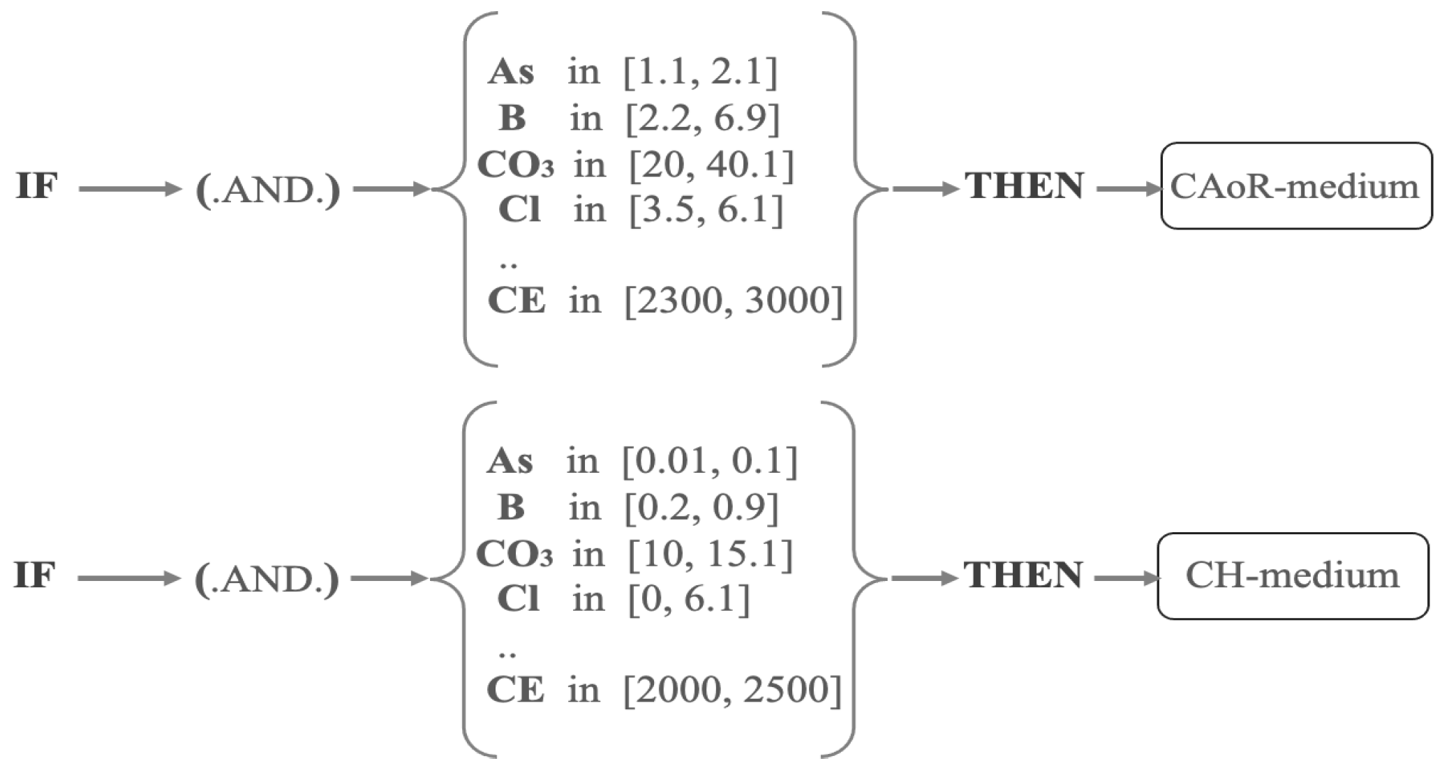
Production rules are as follows: IF <condition> THEN <actions>, where <condition> uses combinations of physicochemical parameters threshold values to give a conclusion. The conclusions correspond to the selection of a label x ∈ {CAoR-Low, CAoR-Medium, CAoR-High, CH-Low, CH-Medium, CH-High}.

3.

Expert validation and testing. For validation, randomly selected records from the different datasets (about 15% from each dataset) were used as input for WQ labels. The result was validated by a disciplinary expert.

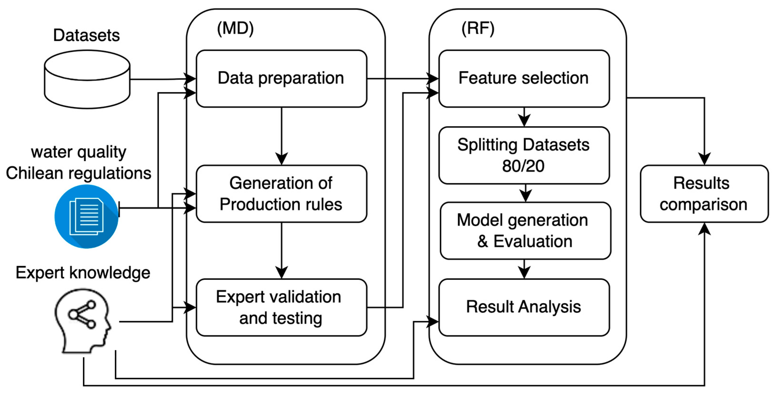
In Figure 2, (MD) shows the steps above. Two examples of production rules are shown in Figure 3.

For the predictive model using RF, relevant physicochemical parameters were selected as predictor variables, a WQ variable being added as the target variable to each dataset.

The methodological stages for generating predictive models at each monitoring point (Table 1) are described below.

• Feature Selection. This stage consisted in filtering and selecting WQ significant predictor variables. Selection criteria were based on expert knowledge and the interpretation of pairwise relationships to identify possible prior dependency relationships between predictor variables. Python was used to identify these types of relationships, particularly the scatter matrix function with the diagonal = “KDE” parameter.
• Splitting Datasets. In this stage, the original data from each of the monitoring points were divided (split) into 80% for training and tuning hyperparameters and 20% for testing the final model to obtain an unbiased estimate. The optimal model was found using K-fold cross-validation with five folds.
• Model Generation and Evaluation. In this stage, the RF models for each monitoring point were generated, and the results of the models were estimated and analyzed to determine their validity. Evaluation consisted in checking the performance of the models obtained with RF for each dataset. To accomplish this, values of certainty, such as accuracy, recall, and precision, were calculated and analyzed. The calculation of these values of certainty and their importance for the model quality are described below.
• Result Analysis. This was performed by analyzing aspects such as how optimal variable parametrization was or how well training set instances were classified (confusion matrix values).

Stages 2, 3, and 4 were designed and conducted similarly to [26,27].

To conduct the validation in stage 4 above, a confusion matrix was obtained for each of the models. This matrix facilitates the analysis to determine where classification errors occur. The confusion matrix is a table showing the error distribution in the four categories: true instances correctly classified (true positives), true instances incorrectly classified (false negatives), false instances correctly classified (true negatives), and false instances incorrectly classified (false positives). Next, the measures of merit of each classifier from previous studies [27] were used similarly.

The measures of merit used in this study help to determine the quality of the predictive models developed and are based on data from the confusion matrix and the result of training with each classification algorithm. These values of merit are as follows:

1. Accuracy (acc) corresponds to the ratio of correctly classified samples from all the samples in the dataset [26,27]. This indicator can be calculated with the confusion matrix data, according to Equation (2), assuming that the dataset is not empty.

acc = (a + d)/(a + b + c + d)

(2)

2. Precision (p) is the proportion of true positives (a) among the elements predicted as positive. Conceptually, precision refers to the dispersion of the set of values obtained from the repeated measurements of a quantity. Particularly, a high precision value (p) implies a low measurement dispersion [26,27]. This indicator can be calculated with Equation (3), assuming (a + b) ≠ 0.

p = (a/a + b) ×100

(3)

3. Recall (r) is the proportion of true positives predicted among the elements classified as positive, that is, the fraction of relevant instances classified [26,27]. Recall can be calculated with Equation (4), assuming (a + c) ≠ 0.

r = (a + d)/(a + c)

(4)

The final task is the comparison of results (Figure 2), which consists in comparing the results obtained from the generation of WQ labels and the results obtained from RF. This comparison focuses on determining the importance of the predictor variables and the number of samples placed in each set for each monitoring point.

Figure 4 shows two examples of scatter matrices of pairwise relationships between predictive variables. To better observe the relationships between variables, the plot was divided into two parts: Part (a) corresponds to the visualization of relationships between the first seven variables (parameters As, B, SO₄, CO₃, Cu, Mg, and Hg), while part (b) corresponds to the visualization of relationships between the remaining variables (parameters NO₃, Pb, Zn, Cl, O₂, pH, and EC).

Parameter As can be deduced from Figure 4 as the parameter least correlated with the rest of the other predictive variables of the datasets, this being particularly true for the relationship between parameters NO₃ and EC.

The relationship between NO₃ and EC can be explained because EC measures water salinity, and, since NO₃ is a salt, thus, the particular correlation between NO₃ and EC makes sense. However, NO₃ can chemically react with other elements, such as Mg, Cl, or even As. Therefore, high NO₃ concentrations could indicate a high presence of fertilizers or contamination by Mg and Cl ions.

Therefore, this parameter was included in the dataset due to the information it can provide. For this reason, these variables were used as predictor variables for the RF model generated in each of the seven datasets shown in Table 1. To generate the models, the free educational version of RapidMiner 9.7^® was used. This software allows developing models with the desired characteristics and available datasets [26,27].

4. Results

Here, pairwise independence was identified between the selected predictive variables. Table 3 shows the WQ ranges for the physicochemical parameters generated for Atacama Desert. These ranges (Table 3a,b) were built using both the criteria established in the Chilean WQ laws, as described in Section 2, and expert knowledge.

Another result is related to the ranges of the independent variables shown in Table 3, which result from the analysis of expert knowledge, available literature, and the WQ standards described in Section 2.3. Supplementary Materials Table S1 shows the descriptive statistics of the WQ physicochemical parameters at the observation points.

Using the ranges of the independent variables described in the previous paragraph, WQ values were generated. These WQ values were used as the dependent variable in the training datasets of WQ predictive models.

RF training was conducted independently with L1, L2, L3, L4, L5, L6, and L7 datasets, using the same algorithm parameter settings. This includes the number of trees = [30, 50, 70, and 100], criterion = [“gain ratio”, “accuracy”, “information gain”, and “Gini index”], maximal depth = 10, and strategy = confidence vote.

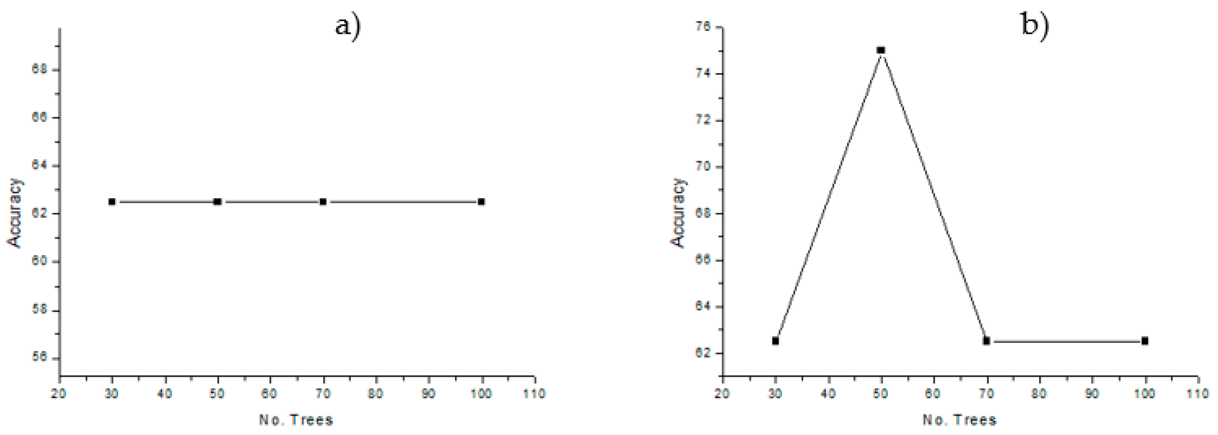
For the training configuration above, a comparative analysis of results was made, as shown in Figure 5, which shows that RF precision is better when “information gain” and “Gini index” are used. A 75% RF-model precision is achieved when the number of trees equals 50.

Here, seven predictive models were generated, using 80% of data for cross-validation and 20% for validation, similar to [27]. Three measures of merit, including acc, p, and r, were used for each algorithm to evaluate the quality of each of these models.

The result of the parameters “classification error” (Cl-Err), Class Precision, acc, p, and r can be observed in

Table 4. Cl-Err and merit values for predictive models.

Dataset	Class Precision	Cl-Err	acc	p	r
L1	98.9910	0.0173	0.8891	89.6631	0.9991
L2	99.9920	0.0142	0.9993	94.8289	1.0000
L3	100.0000	0.0703	0.9987	97.3427	1.0000
L4	99.9970	0.0159	0.9891	96.8731	1.0000
L5	99.4430	0.0369	0.9957	91.5359	1.0000
L6	93.6570	0.0407	0.9899	98.1137	1.0000
L7	99.8950	0.0077	0.9778	91.4342	1.0000

, showing that the classification precision for all the models is over 98.80%, while the ideal classification precision is 100%. The mean value of acc = 0.9770 indicates that almost all the samples in the datasets were correctly classified, while the worst absolute value in all the models was obtained for dataset L1.

Similarly, the mean value of p = 94.2559 indicates a reasonable medium dispersion value for all datasets, while the worst absolute value of p in all the models was obtained for dataset L1.

The low value of p for dataset L1 may be associated with high data dispersion in this dataset, different than the remaining datasets. The average value of r = 0.9998 indicates that the proportion of true positives predicted from the classified elements is very good and close to 100%.

In each dataset, the threshold values (Supplementary Materials Table S1) can be compared and better adapted to the context of the Loa River section studied here. This means that the threshold value ranges for the predictor variables may be further adjusted to the context of the Loa River section where the RF model was generated. In this way, predictions made can be better contextualized.

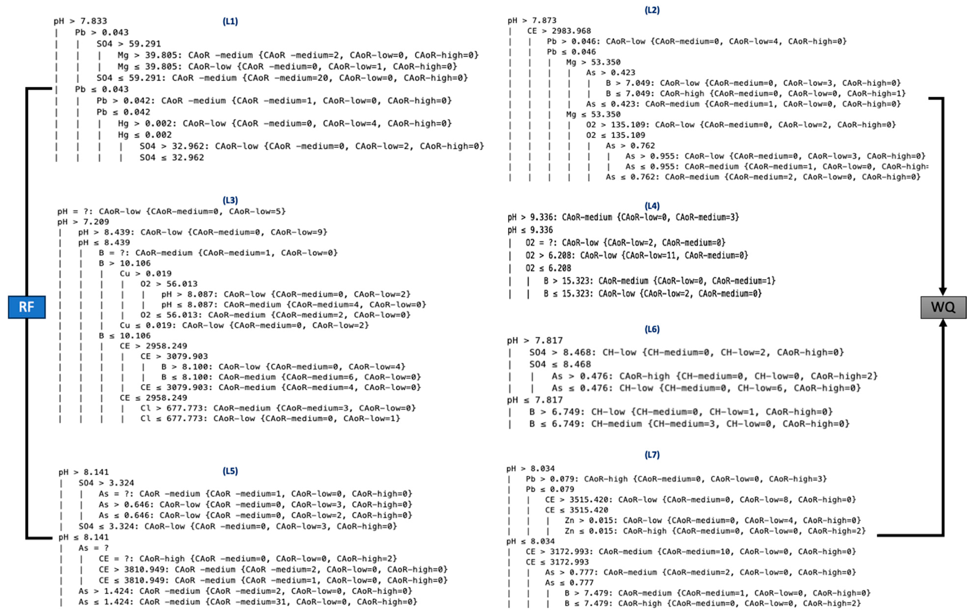
Figure 6 shows seven tree structures constructed using RF. Each section of the figure represents a selected tree where the principal node (root node) is pH, the important threshold values of parameters being related.

In detail, the tree in L1 indicates that “CAoR-Medium” values can be assigned when pH > 7.510 and parameter Pb > 0.020 and B > 8.157. Similarly, the tree in L2 indicates that “CAoR-Low” values can be assigned when pH > 7.873, CE > 2983, and Pb > 0.046.

A pH value similar to the root node is shown in L6 and L7 trees. The tree in L7 indicates that the “CAoR-High” value can be assigned when pH > 7.873 and CE ≤ 2903.465; the tree in L6 indicates that the “CAoR-High” value can be assigned when pH > 7.873 and CE ≤ 2903.465. These pH threshold values shown in the RF trees contrast with the previous ones calculated by expert experience and the regulation described in Section 2.3 (Table 3).

On the other hand, this contrasts with the range described in Table 3 for parameters such as B, Pb, and As, which were calculated by expert knowledge and using the description in Section 2.3. For example, the RF tree in L7 indicates that the “CAoR-Medium” value can be assigned when As ≤ 0.777, but it does not correspond to values in the minimum–maximum range in the Chilean regulation [31,32] (Table 2).

So, these results do not contradict WQ regulations in Section 2.3; however, they could be used for a classification further adapted to the context of the Loa River basin. Interpretations based on trees obtained with RF allow creating new ranges to classify new data arriving at the datasets from the different observation points. For example, the values of B should be in the range (12.382, 15.138), or the values of SO₄ should be in the range (0.1, 3.324), as shown in the RF tree of L5.

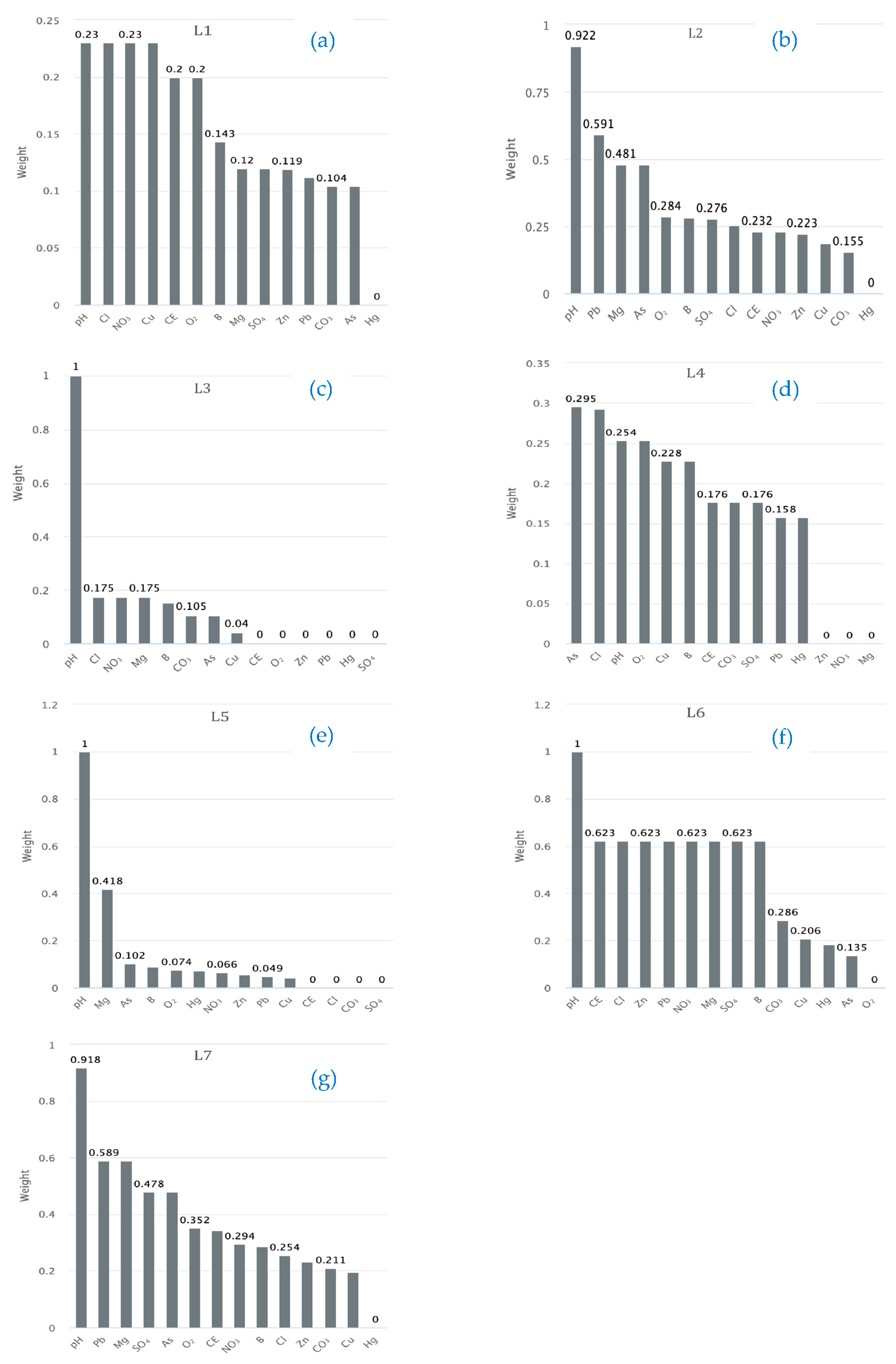
For each RF model, the most significant predictive variables (according to the Weight by Information Gain Ratio metric) were calculated, as shown in Figure 7. In this figure, a, b, c, d, e, f, and g correspond to the L1, L2, L3, L4, L5, L6, and L7 monitoring stations, respectively.

Six of the seven figures show that the physicochemical parameter pH is the most significant. Only in Figure 7d, parameter As is the most significant, followed by Cl and then pH. So, parameter (pH) predominates in all datasets when determining the WQ value. Similarly, parameter Cl is present as a significant variable in four of the seven graphs, while parameters As, Pb, and Cl appear as significant variables in three of the seven graphs.

The other parameters are repeated two or fewer times, as shown in Figure 7. In this case, some parameters were not relevant in some of the models, such as the one for L3 (Figure 7c), where parameters EC, O₂, Zn, Pb, Hg, and SO₄ were not significant. For future predictions using the RF model, it would be sufficient to have values of the other parameters that represent 64% of the data to be acquired.

To ensure optimal selection, only the five most significant physicochemical parameters were considered for the outlier validation of each model. Box-plot graphs shown in Figure 8 were generated using Python 3.11 for this purpose.

This task aimed to determine how much the sample mean could be affected by the presence of outliers, as this could have an impact on the conclusions drawn from each model. To reinforce this technique, the Interquartile Range (IQR) value was calculated for the most significant variable. IQR is related to outliers, as it is sensitive to the dispersion that may exist in each sample mean [33]. Both the graphs and IQR values were interpreted, their impact on the model being described below. Figure 8 shows that the most significant variables in each group contain few outliers.

In Figure 8, starting from the third most significant variable in the group of five variables, outliers begin to appear, suggesting that a good refinement to validate the quality of variable selection could be reducing the selection from five to the three most significant variables. This is reinforced by IQR indices: 0.351250, 0.412499, 0.557500, 0.241500, 0.342500, 0.415000, and 0.389999 for variables pH (from L1), pH (from L2), pH (from L3), As (from L4), pH (from L5), pH (from L6), and pH (from L7), respectively.

The IQR values are relatively low, the highest one corresponding to the most significant variable of L3, i.e., pH with a value of 0.557500. This can be interpreted as all models having a low impact of outliers.

Therefore, the RF method generates good models that can be used for new cases, given the level of certainty of the model quality and the verification of outliers described above. A limitation of this study is that the model was trained with data from only seven water quality monitoring stations in the Loa River basin, despite DGA monitoring more than 50 points in this basin.

5. Conclusions

This paper describes a novel method to identify the significant values of physicochemical parameters and heavy-ion metals, and also significant ranges of these physicochemical parameters and heavy-ion metals in an extremely arid desert environment. Interestingly, these ranges perfectly fit the Loa River basin characteristics. The method generates representative labels for Loa River geochemical characteristics. These labels are used to classify water quality into two large groups: for human and animal consumption and for irrigation. For each group below, three water quality labels were created.

Threshold values and expert knowledge were used to generate production rules to obtain threshold values for physicochemical parameters perfectly adapted to the characteristics of the Loa River section studied. Therefore, these values are significant for future studies in this extremely arid zone of Atacama Desert. In addition, this study considered recent research using machine learning techniques to generate predictive models for water quality. In this way, a technique that can be used in other contexts was developed to generate significant ranges for particular physicochemical parameters and water quality labels thoroughly adjusted to this particular context.

Additionally, this paper describes a novel approach using Random Forest to develop a water quality prediction model not considering the Water Quality Index. Instead, the model is based on: (1) historical data on physicochemical parameters in a region characterized by high aridity, mineral concentration, and water resources for sustaining the Atacama Desert ecosystem; (2) Chilean WQ regulations; and (3) expert knowledge. The RF model generation process allows further understanding physicochemical parameters and their influence on WQ for human and livestock consumption and for agricultural purposes. Both aspects of water use focus on the characteristics and particularities of the Loa River basin.

The RF model allows generating low, medium, or high WQ labels, which can be compared with those obtained in the first part of this study, to answer the research question and validate the RF model usefulness. The resulting models were validated using the cross-validation method. This allowed developing validated and reliable models for all the monitoring stations, with a minimal error value in training, resulting in over 96% average accuracy for all the predictive WQ models, using the seven datasets prepared for this study, and over 97% average precision for all the classifier training.

Moreover, measures of merit (acc, p, r) for each classifier were used to determine the quality of the predictive models developed. In this context, the models obtained show the following mean values: acc = 0.897, p = 89.73, r = 0.928. These values show good results. The results obtained with RF could be used to apply the same methodology and obtain threshold values for the parameters considered here. As stated above, these values are particular for the study domain and directly associated with Loa River quality.

A future line of research could involve adapting the models obtained at each of these physicochemical parameter observation points to other hydrometric stations in the Loa River basin, along with making WQ predictions to support tasks such as studying the possible environmental impact of the parameters studied here or validating parameters of interest to determine Loa River WQ. This study could be replicated in river basins on different geochemical conditions, generalizing the technology created here to develop predictive models adapted to different geochemical contexts.

References

1. Muñoz-Farías, S.; Ritter, B.; Dunai, T.J.; Morales-Leal, J.; Campos, E.; Spikings, R.; Riquelme, R. Geomorphological significance of the Atacama Pediplain as a marker for the climatic and tectonic evolution of the Andean forearc, between 26° to 28° S. Geomorphology 2023, 420, 108504. [Google Scholar] [CrossRef]
2. Alnahit, A.O.; Mishra, A.K.; Khan, A.A. Quantifying climate, streamflow, and watershed control on water quality across Southeastern US watersheds. Sci. Total Environ. 2020, 739, 139945. [Google Scholar] [CrossRef] [PubMed]
3. Muharemi, F.; Logofătu, D.; Leon, F. Machine learning approaches for anomaly detection of water quality on a real-world data set. J. Inf. Telecommun. 2019, 3, 294–307. [Google Scholar] [CrossRef] [Green Version]
4. Huang, H.; Lu, J. Identification of river water pollution characteristics based on projection pursuit and factor analysis. Environ. Earth Sci. 2014, 72, 3409–3417. [Google Scholar] [CrossRef]
5. USEPA. Parameters of Water Quality: Interpretation and Standards; Environmental Protection Agency: Wexford, Ireland, 2001. [Google Scholar]
6. Méndez, M.; Prieto, M.; Godoy, M. Production of subterranean resources in the Atacama Desert: 19th and early 20th-century mining/water extraction in The Taltal district, northern Chile. Political Geogr. 2020, 81, 102194. [Google Scholar] [CrossRef]
7. Kereszturi, Á. Unique and potentially Mars-relevant flow regime and water sources at a high Andes-Atacama site. Astrobiology 2020, 20, 723–740. [Google Scholar] [CrossRef]
8. Tapia, J.; González, R.; Townley, B.; Oliveros, V.; Álvarez, F.; Aguilar, G.; Calderón, M. Geology and geochemistry of the Atacama Desert. Antonie Leeuwenhoek 2018, 111, 1273–1291. [Google Scholar] [CrossRef]
9. Arias-Carrasco, R.; Rojas-Herrera, M.; Sepúlveda-Hermosilla, G.; Maracaja-Coutinho, V.; Huanca-Mamani, W.; Cárdenas-Ninasivincha, S.; Bastáas, E. Long Non-Coding RNAs Responsive to Salt and Boron Stress in the Hyper-Arid Lluteno Maize from Atacama Desert. Genes 2018, 9, 170. [Google Scholar]
10. Arriaza, B.; Amarasiriwardena, D.; Starkings, J.; Ogalde, J.P. Use of LA-ICP-MS to evaluate mercury exposure or diagenesis in Inca and non-Inca mummies from northern Chile. Archaeol. Anthropol. Sci. 2022, 14, 76. [Google Scholar] [CrossRef]
11. Bull, A.T.; Asenjo, J.A. Microbiology of hyper-arid environments: Recent insights from the Atacama Desert, Chile. Antonie Leeuwenhoek 2013, 103, 1173–1179. [Google Scholar] [CrossRef]
12. Flores-Varas, A.; Heine-Fuster, I.; López-Allendes, C.; Pizarro, H.; Castro, D.; Luque, J.A.; Aránguiz-Acuña, A. Ascotán, and Carcote salt flats as sensors of humidity fluctuations and anthropic impacts in the transition zone of the Andean Altiplano. J. S. Am. Earth Sci. 2021, 105, 102934. [Google Scholar] [CrossRef]
13. Pino-Vargas, E.; Chavarri-Velarde, E. Evidence of climate change in the hyper-arid region of the southern coast of Peru, head of the Atacama Desert. Tecnol. Cienc. Agua 2022, 13, 333–375. [Google Scholar] [CrossRef]
14. Díaz, F.P.; Latorre, C.; Carrasco-Puga, G.; Wood, J.R.; Wilmshurst, J.M.; Soto, D.C.; Gutiérrez, R.A. Multiscale climate change impacts on plant diversity in the Atacama Desert. Glob. Chang. Biol. 2019, 25, 1733–1745. [Google Scholar] [CrossRef] [PubMed]
15. Wang, Z.; Wei, J.; Peng, W.; Zhang, R.; Zhang, H. Contents and spatial distribution patterns of heavy metals in the hinterland of the Tengger Desert, China. J. Arid. Land. 2022, 14, 1086–1098. [Google Scholar] [CrossRef]
16. Vargas-Machuca, B.D.; Zanetta-Colombo, N.; De Pol-Holz, R.; Latorre, C. Variations in local heavy metal concentrations over the last 16,000 years in the central Atacama Desert (22° S) measured in rodent middens. Sci. Total Environ. 2021, 775, 145849. [Google Scholar] [CrossRef]
17. Yang, L.; Ma, X.; Luan, Z.; Yan, J. The spatial-temporal evolution of heavy metal accumulation in the offshore sediments along the Shandong Peninsula over the last 100 years: Anthropogenic and natural impacts. Environ. Pollut. 2021, 289, 117894. [Google Scholar] [CrossRef]
18. López-Berenguer, G.; Pérez-García, J.M.; García-Fernández, A.J.; Martínez-López, E. High levels of heavy metals detected in feathers of an avian scavenger warn of a high pollution risk in the Atacama Desert (Chile). Arch. Environ. Contam. Toxicol. 2021, 81, 227–235. [Google Scholar] [CrossRef]
19. Moreno, M.L.; Piubeli, F.; Bonfá, M.R.L.; García, M.T.; Durrant, L.R.; Mellado, E. Analysis and characterization of the cultivable extremophilic hydrolytic bacterial community in heavy-metal-contaminated soils from the Atacama Desert and their biotechnological potentials. J. Appl. Microbiol. 2012, 113, 550–559. [Google Scholar] [CrossRef]
20. Lintern, A.; Webb, J.A.; Ryu, D.; Liu, S.; Bende-Michl, U.; Waters, D.; Leahy, P.; Western, A.W. Key factors influencing differences in stream water quality across space. Wiley Interdiscip. Rev. Water 2018, 5, e1260. [Google Scholar] [CrossRef] [Green Version]
21. Abuzir, S.Y.; Abuzir, Y.S. Machine learning for water quality classification. Water Qual. Res. J. 2022, 57, 152–164. [Google Scholar] [CrossRef]
22. Ahmed, A.N.; Othman, F.B.; Afan, H.A.; Ibrahim, R.K.; Fai, C.M.; Hossain, M.S.; Ibrahim, R.K.; Fai, C.M.; Hossain Md Ehteram, M.; Elshafie, A. Machine learning methods for better water quality prediction. J. Hydrol. 2019, 578, 124084. [Google Scholar] [CrossRef]
23. Gayen, A.; Pourghasemi, H.R.; Saha, S.; Keesstra, S.; Bai, S. Gully erosion susceptibility assessment and management of hazard-prone areas in India using different machine learning algorithms. Sci. Total Environ. 2019, 668, 124–138. [Google Scholar] [CrossRef]
24. Plazas-Nossa, L.; Ávila Angulo, M.A.; Torres, A. Detection of outliers and imputing of missing values for water quality UV-Vis absorbance time series. Ingeniería 2017, 22, 111–124. [Google Scholar] [CrossRef]
25. Avila-Perez, H.; Flores-Munguía, E.J.; Rosas-Acevedo, J.L.; Gallardo-Bernal, I.; Ramirez-delReal, T.A. Comparative Analysis of Water Quality Applying Statistic and Machine Learning Method: A Case Study in Coyuca Lagoon and Tecpan River, Mexico. Water 2023, 15, 640. [Google Scholar] [CrossRef]
26. Flores, V. Determination of Trees Predictive Models for Surface Roughness in High-Speed Machining (HSP): A Study in Steel and Aluminum Metalworking Industry. In Research Highlights in Mathematics and Computer Science; BP International: Karuppur, India, 2023; Volume 4, pp. 42–66. [Google Scholar]
27. Flores, V.; Keith, B. Gradient boosted trees predictive models for surface roughness in high-speed milling in the steel and aluminum metalworking industry. Complexity 2019, 2019, 1536716. [Google Scholar] [CrossRef] [Green Version]
28. Zanetta-Colombo, N.C.; Fleming, Z.L.; Gayo, E.M.; Manzano, C.A.; Panagi, M.; Valdés, J.; Siegmund, A. Impact of mining on the metal content of dust in indigenous villages of northern Chile. Environ. Int. 2022, 169, 107490. [Google Scholar] [CrossRef]
29. Ruffino, B.; Campo, G.; Crutchik, D.; Reyes, A.; Zanetti, M. Drinking Water Supply in the Region of Antofagasta (Chile): A Challenge between Past, Present and Future. Int. J. Environ. Res. Public Health 2022, 19, 14406. [Google Scholar] [CrossRef]
30. Min, D.H.; Yoon, H.K. Suggestion for a new deterministic model coupled with machine learning techniques for landslide susceptibility mapping. Sci. Rep. 2021, 11, 6594. [Google Scholar] [CrossRef]
31. INN-NCh409; Official Chilean Drinking Water Standard. National Institute for Standardization. INN: Santiago, Chile, 2005.
32. INN-NCh1333; Official Chilean Standard NCh1333 Water Quality Requirements for Different Uses. INN, National Institute for Standardization: Santiago, Chile, 1987.
33. Dritsas, E.; Trigka, M. Efficient Data-Driven Machine Learning Models for Water Quality Prediction. Computation 2023, 11, 16. [Google Scholar] [CrossRef]
34. Alnahit, A.O.; Mishra, A.K.; Khan, A.A. Stream water quality prediction using boosted regression tree and random forest models. Stoch. Environ. Res. Risk Assess. 2022, 36, 2661–2680. [Google Scholar] [CrossRef]
35. Mori, T. Information gain ratio as term weight: The case of summarization of ir results. In Proceedings of the En Coling 2002: The 19th International Conference on Computational Linguistics, Taipei, Taiwan, 24 August–1 September 2002. [Google Scholar]
36. Johansson, C.; Zhang, Z.; Engardt, M.; Stafoggia, M.; Ma, X. Improving 3-day deterministic air pollution forecasts using machine learning algorithms. Atmos. Chem. Phys. Discuss. 2023; preprint. [Google Scholar]
37. Zhu, M.; Wang, J.; Yang, X.; Zhang, Y.; Zhang, L.; Ren, H.; Bing, W.; Ye, L. A review of the application of machine learning in water quality evaluation. Eco-Environ. Health 2022, 1, 107–116. [Google Scholar] [CrossRef]
38. Molina, M.; Flores, V. A knowledge-based approach for automatic generation of summaries of behavior. In Proceedings of the Artificial Intelligence: Methodology, Systems, and Applications: 12th International Conference, AIMSA 2006, Varna, Bulgaria, 12–15 September 2006; Springer: Berlin/Heidelberg, Germany, 2006. [Google Scholar]
39. Legasa, M.N.; Manzanas, R.; Calviño, A.; Gutiérrez, J.M. A posteriori random forests for stochastic downscaling of precipitation by predicting probability distributions. Water Resour. Res. 2022, 58, e2021WR030272. [Google Scholar] [CrossRef]
40. Regier, P.; Duggan, M.; Myers-Pigg, A.; Ward, N. Effects of random forest modeling decisions on biogeochemical time series predictions. Limnol. Oceanogr. Methods 2023, 21, 40–52. [Google Scholar] [CrossRef]
41. Herrera, C.; Godfrey, L.; Urrutia, J.; Custodio, E.; Jordan, T.; Jódar, J.; Barrenechea, F. Recharge and residence times of groundwater in hyper-arid areas: The confined aquifer of Calama, Loa River Basin, Atacama Desert, Chile. Sci. Total Environ. 2021, 752, 141847. [Google Scholar] [CrossRef] [PubMed]
Figure 1. Study area.
Water 15 02868 g001
Figure 2. WQ prediction methodology using real data and RF.
Water 15 02868 g002
Figure 3. Examples of production rules in the domain.
Water 15 02868 g003
Figure 4. Example of a scatter matrix of pairwise relationships between predictor variables.
Water 15 02868 g004
Figure 5. (a) “Gain ratio” and “accuracy” results; (b) “Information gain” and “gini index” results.
Water 15 02868 g005
Figure 6. Tree structures constructed with RF.
Water 15 02868 g006
Figure 7. Bar charts of predictor variables at each monitoring station. Variable weights estimated using Weight by Information Gain Ratio metric. Graphs (ag) correspond to the L1, L2, L3, L4, L5, L6, and L7 monitoring stations, respectively.
Water 15 02868 g007
Figure 8. Most significant WQ parameters at Loa River basin locations. Figure 8 shows box-plots as follows: Graph (a): pH, Cl, NO3, CU, and CE for L1; Graph (b): pH, Pb, Mg, As, and O2 for L2; Graph (c): pH, Cl, NO3, B, and CO3 for L3; Graph (d): As, Cl, pH, O2, and Cu for L4; Graph (e): pH, Mg, As, B, and O2 for L5; Graph (f): pH, CE, Cl, Zn, and Pb for L6; and Graph (g): pH, Pb, Mg, SO4, and As for L7.
Water 15 02868 g008