Evaluation of Legacy Forest Harvesting Impacts on Dominant Stream Water Sources and Implications for Water Quality Using End Member Mixing Analysis

Abstract

Forests are critical water supply regions that are increasingly threatened by natural and anthropogenic disturbance. Evaluation of runoff-generating processes within harvested and undisturbed headwater catchments provides insight into disturbance impacts on water quality and drinking water treatability. In this study, an extensive hydrologic dataset collected at the experimental Turkey Lakes Watershed (TLW) located on the Canadian Shield was used to quantify sources of stormflow in legacy clear-cut (24-years post harvesting) and forested (control) headwater catchments using an end member mixing analysis (EMMA) model. Stream water, groundwater, soil water, and throughfall water quality were evaluated during spring snowmelt, stormflow, and fall wet-up. Groundwater chemistry was similar to stream water chemistry in both catchments, suggesting that groundwater is a major contributor to stream flow. The water chemistry in small wetlands within the study catchments was comparable to stream water chemistry, suggesting that wetlands are also important contributors to stream flow. Differences in wetland position between the legacy clear-cut and control catchments appeared to have a greater influence on source contributions than legacy harvesting. Results from this study provide insight into runoff-generation processes that reflect event/seasonal flow dynamics and the impacts on water quality.

1. Introduction

Forested landscapes are critical for the provision of safe and reliable drinking water to a majority of Canadians and 60% of the U.S. population, and 60% of the world’s largest cities also rely on forests for water [1,2,3,4]. The ecosystem services of tropical and temperate forests have been valued at USD 23.32 trillion per year [5,6], with savings to global drinking water treatment costs valued at USD ~4.1 trillion per year [7]. Landscape disturbance threatens water supply through alterations to hydrologic and biogeochemical cycles that ultimately change water quantity and quality; these threats are further exacerbated by compound disturbance (e.g., heavy precipitation following wildfire) [1,8,9]. Forest disturbance typically intensifies the water cycle, resulting in more water moving through the landscape [10,11], which increases the transport of sediment and nutrients to stream channels [9,12,13,14]. Sediment and nutrients are transported downstream [15,16,17] and challenge drinking water treatment operations [1]. However, the varied hydrologic responses of forested catchments to landscape disturbance [18,19,20,21] make predicting disturbance effects difficult [22]. Explaining this variability requires an understanding of the impacts of landscape disturbance on water movement and storage in a variety of forested landscapes [20,22,23] and is essential to evaluate potential risks to drinking water treatment operations [1,22].

Harvesting of trees is a common anthropogenic disturbance in many forested ecosystems [24]. In addition to industrial forestry and silviculture, harvesting is increasingly advocated as a techno-ecological nature-based solution (TE-NBS) [25] for mitigating climate-change-exacerbated landscape disturbance (e.g., wildfire) threats to drinking water treatability [25,26]. Critically, however, harvesting can impact water storage and flow paths. Vegetation removal associated with harvesting can reduce rates of precipitation interception and transpiration and increase the water content of forest soils [11,27,28]. Additionally, heavy equipment can change the physical characteristics of forest soils by increasing soil bulk density and reducing soil porosity and infiltration rates [29,30,31,32]. These changes may increase soil saturation [33,34] and reduce the water-storage capacity of soils after harvesting [35,36]. Reduced water-storage capacity can increase the proportion of water transported via overland flow [29] and shallow subsurface pathways [37,38] that result in more frequent, quick flow events [36,39]. Notably, these combined changes result in higher annual and seasonal water yields [10,40] and increased peak flows [11].

Long-term experimental watersheds such as the Turkey Lakes Watershed (TLW) in Ontario, Canada, provide detailed historical hydro-chemical data that can be used to evaluate complex hydrological processes [41]. Previous work at TLW has shown that shallow soil water is a major contributor to stream flow during snowmelt [42] and that perched water tables over less permeable/impermeable soil layers direct flow through the upper soil profile [43]. Threshold relationships were observed between quick flow and precipitation [36], and stream flow generation is controlled through transmissivity feedback (rapid stream flow increases as the water table approaches soil surfaces) [38]. A forest harvesting experiment conducted at TLW showed that harvesting increased the proportion of water moving through the upper soil profile [10,38], reduced mean water travel times [23,37], and decreased the root-zone-storage capacity, resulting in a reduced precipitation threshold required for quick flow production [36]. Accordingly, increased instances of annual and seasonal water yields draining harvested catchments were observed, with some signs of recovery 15 years after harvesting [10]. Collectively, this work described key impacts of forest harvesting on hydrologic response during the first 15 years post harvest. However, few studies have been conducted to evaluate the longer-term (>20 years) legacy impacts of forest harvesting on hydrologic processes that control stream flow generation. [10,13,44].

End member mixing analysis (EMMA) is a commonly used tool that attempts to explain observed stream water chemistry composition as a mixture of different source areas or “end members”, assuming a linear mixing process [45,46,47,48]. End members are pre-defined hydrologic source areas such as groundwater, soil water, precipitation, and snowmelt that are hypothesized to contribute water to stream flow. The dimensionality of stream water chemistry datasets is removed using principal component analysis (PCA), and potential end members are projected into the mixing subspace defined by the stream water chemistry [46,49]. End members are then evaluated for their ability to explain stream water chemistry in the mixing subspace, and mass balance equations are used to calculate relative end member contributions to stream flow [46,48]. Diagnostic tools using eigenvector and residual analysis have been developed to estimate the number of end members required to explain the stream water chemistry without prior knowledge of the existing end members [50].

EMMA has provided numerous insights regarding runoff-generation processes and water quality. Many studies define end members differently, making direct comparisons difficult [51]. However, other studies have demonstrated that three end members are often sufficient to explain stream water chemistry [48,52] and that the prominent end member contributing to stream water can change depending on antecedent soil moisture conditions [48,53]. For example, at the Panola Mountain Research Watershed in Georgia, USA, end member contributions to stream flow changed from outcrop runoff to riparian groundwater with increasing antecedent moisture conditions [53]. Similarly, the number of end members contributing to stream flow increased from two to three under higher antecedent moisture conditions, as the transient saturated groundwater end member was only contributing to stream flow under wet antecedent moisture conditions in the Kiryu Experimental Watershed, Japan [52].

Additional insights into how changing end members contributes to water quality have also been assembled. For example, snowmelt was reported to drive episodic acidification within stream water by diluting base cations at the Hubbard Brook Experimental Forest in New Hampshire, USA [54]. This dilution effect shifted during summer storms as the end member contributions from upper soil horizons became more prominent and supplied organic acids to the stream channel [54]. At the H.J. Andrews Experimental Forest in Oregon, USA, EMMA was used to identify lateral subsurface flow originating from the organic and upper soil horizons as the dominant end member contributing dissolved organic carbon (DOC) and dissolved organic nitrogen (DON) to the stream network during the rising limb of the hydrograph [55]. These studies highlight the utility of EMMA for discerning end member contributions to stream water under different antecedent soil moisture conditions and subsequent impacts on water quality. However, few studies have utilized EMMA to evaluate landscape disturbance impacts on runoff-generation processes or inform the suitability of forest harvesting as a source-water-protection strategy.

This study presents the results from an intensive field sampling program that characterized the water chemistry of multiple end members contributing to stream flow in legacy clear-cut and forested control catchments on the Canadian Shield. Increased knowledge of these runoff-generation processes is critical to explaining water quality responses to landscape disturbance. The specific objectives of this study were to (1) assess the primary end member contributions to stream flow in a legacy clear-cut (>20 years post harvest) and unharvested (control) catchments using end member mixing analysis and (2) assess temporal variability in end member contributions to stream flow during spring snowmelt, summer storm events, and fall wet-up.

2. Materials and Methods

2.1. Study Site

The Turkey Lakes Watershed (TLW; 47°03′ N; 84°25′ W) is an experimental watershed located in the Great Lakes in the St. Lawrence Forest Region of central Ontario (Figure 1). The watershed drains an area of 10.5 km², and the relief is ~300 m [41,43]. From 1980 to 2017, the mean annual temperature and precipitation was 4.5 °C and 1203 mm, respectively, with ~35% of annual precipitation falling as snow [41,43]. The bedrock consists of Precambrian silicate greenstone (i.e., metamorphic basalt), with outcroppings of felsic igneous rock [41,56]. Overlying the bed rock is a two-component glacial till consisting of a compacted sandy basal till underlying a silt–loam ablation till [42,43]. Soils are classified as ortho humic–ferric podzols (spodosols), with well-defined L and F horizons typically 0.05 m thick [57]. The forest comprises predominantly uneven-aged, shade-tolerant, mature to over-mature hardwoods [56]. Sugar maple (Acer saccharum Marsh) comprises 90% of tree species, with yellow birch (Betula alleghaniensis Britton) and assorted conifers representing 9% and 1% of tree species, respectively [43,56].

2.2. Experimental Design

This study was conducted in two headwater sub-catchments within TLW. Catchment 31 (C31) has an area of 4.9 ha, total relief of 80 m, and a wetland area of ~2.0%. Catchment 32 (C32) has an area of 6.6 ha, total relief of 107 m, and a wetland area of ~1.5% [13]. In the fall of 1997, a silvicultural harvesting experiment was conducted in C31 to evaluate the effects of forest harvesting on soil productivity, stand recovery, biodiversity, and water quantity and quality [10]. C31 was treated with a diameter-limited or clear-cut harvesting strategy, which involved the felling and removal of all trees with a diameter at breast height (DBH) ≥ 20 cm. All trees with a DBH between 10 and 20 cm were felled and left on site, while trees with a DBH ≤ 10 cm were left standing [10,23]. Harvesting resulted in a 78% and 76% reduction in the stocking and basal area, respectively [36]. It should be noted that clear-cut harvesting is not a recommended harvesting strategy for Ontario’s shade-tolerant hardwood forests [58] but was selected to represent an extreme disturbance event [59]. C32 was not harvested to act as control because of its proximity and similar biophysical characteristics to C31. One notable difference between the two catchments is the position of the small, cryptic-treed wetlands (i.e., forested swamps) relative to the catchment outlet [60]. In C31, the wetland is in the upper parts of the catchment near the stream initiation point, whereas in C32, the wetland is located directly above the catchment outlet (Figure 1).

2.3. Field Methods

2.3.1. Flow and Stream Water Chemistry

C31 and C32 were instrumented with 90° v-notch weirs, stilling wells, and Steven’s Smart PT SDI-12™ pressure and temperature transducers to estimate stream flow at the basin outlet every 10 min. Stage–discharge rating curves were used to calculate instantaneous discharge. In addition, level loggers were placed in the upper parts of the stream channel near stream-initiation points. In C31, the stream originates from a small wetland referred to as C31 wetland, and in C32, the stream starts at the bottom of a hillslope referred to as the C32 initiation point. At these sampling locations, only the stream stage was recorded, as creating a stage–discharge rating curve was not possible due to the stream channel size and logistical constraints. Stream water samples were collected at both outlets and the two stream-initiation points using ISCO 6700 automated water samplers and stored in acid-washed, triple-rinsed 1 L polypropylene sampling bottles. ISCO samplers were programmed to collect daily composite (4 times a day) water samples during snowmelt and fall sampling periods. Additionally, the rising and falling limbs of select summer storms were sampled with ISCO samplers programmed to collect a sample every 0.5 to 2 h depending on the predicted size and length of the storm. Five storms were sampled during the summer. Finally, monthly water samples were collected by hand with 500 mL HDPE sampling bottles at all sampling locations to characterize baseflow conditions. All sampling bottles were acid-washed and triple-rinsed before being used in the field.

2.3.2. Groundwater

The ablation and basal till groundwater end member chemistry was characterized by collecting water samples from piezometer nests [37,38]. Piezometer nests consisted of two drive-point piezometers (Solinst Canada Ltd., Georgetown, ON, Canada) with 10 or 25 cm screens and an inside diameter (i.d.) of 2 or 4 cm, which were driven into the ablation or basal till [38]. Each catchment was instrumented with a total of 12 piezometer nests in two transects located in the upper and lower parts of the catchments. Each transect ran perpendicular to the stream channel, with three piezometer nests located on each side of the channel. Average depths of the piezometers were 0.45 ± 0.05 m and 0.40 ± 0.03 m in the ablation till and 1.09 ± 0.19 m and 0.93 ± 0.09 m in the basal till in C31 and C32, respectively [38]. In addition, wetland groundwater was characterized by a single transect of 4 cm i.d. piezometers installed to an average depth of 0.39 ± 0.03 m and 0.37 ± 0.03 m into the wetlands of C31 and C32, respectively. Groundwater samples collected using a peristaltic pump were obtained weekly during the snowmelt and fall sampling periods and during each storm event. Groundwater samples were also collected once per month during the summer to characterize groundwater chemistry during summer baseflow. Piezometers were purged for five minutes or until dry and then sampled the next day to allow the basal till piezometers sufficient time to recharge [37].

2.3.3. Soil Water

Soil pits with two zero-tension lysimeters were installed to collect soil water flowing through the soil profile next to each piezometer nest (excluding wetlands). Soil pits were dug by hand to an average depth of 0.65 ± 0.10 m and 0.64 ± 0.10 m in C31 and C32, respectively. Lysimeters were installed directly below the LFH layer and 20 cm below the LFH mineral soil interface. Lysimeter construction consisted of PVC pipe (15.23 cm i.d.), PVC sheeting, and a plastic screen mesh over the top to create a contact point between the lysimeter and soil/LFH layer. Additionally, the mineral soil lysimeters had glass wool, and a mixture of soil and deionized water was placed on top of the plastic screen mesh to strengthen the contact between the lysimeter and the soil matrix. Water drained from the lysimeters into acid-washed, triple-rinsed 1 L HDPE plastic sampling bottles. Sample bottles were placed in a plastic tote within each soil pit to protect them from the elements. All lysimeters were installed in the fall of 2020 to allow six months to equilibrate with the soil profile before sample collection in the spring of 2021. Two of the soil pits were completely saturated, preventing the installation of the lysimeters. As these soil pits were in small depressions, a drive-point piezometer was installed to a depth of 20 cm approximately one meter upslope of the soil pit to sample water flowing through the upper parts of the soil profile. Soil water samples were collected once a week during the snowmelt and fall sampling period and after each storm event. Fresh sampling bottles were placed in the soil pits before each storm to ensure any sample collected was representative of each storm. Lysimeter samples were also collected once a month in the summer corresponding with the groundwater sampling described above.

2.3.4. Throughfall

A throughfall collector was installed in each catchment to characterize precipitation chemistry. These collectors were constructed from plastic funnels with a mesh zip tied over the top to prevent clogging from leaf litter. The funnel was placed on a steel post next to a soil pit with a sample line running from the funnel to a 1 L HDPE sampling bottle within the tote containing the lysimeter sample bottles. Throughfall water samples were collected under the same sampling schedule as the lysimeters described above.

2.4. Laboratory Methods

All water samples were analyzed at the accredited Water Chemistry Laboratory in the Great Lakes Forestry Centre of the Canadian Forest Service in Sault Ste. Marie, Ontario, Canada. Water samples were analyzed for SO₄²⁻, Ca²⁺, K⁺, Mg²⁺, Na⁻, Al³⁺, Ba²⁺, Sr²⁺, and DOC using standardized procedures and quality control methods [61]. Water chemistry tracers were selected based on tracers used in previous EMMA studies [48,49,53,54]. Due to the COVID-19 pandemic, there were several closures of the water chemistry laboratory, requiring sample freezing and storage for up to four months before processing and analysis could be completed.

2.5. End Member Mixing Analysis Model

End members used in EMMA model were selected based on physical characteristics of the catchments, existing monitoring equipment, and a prior understanding of the hydrological processes within TLW [23,37,38,43,60]. The specific end members selected included basal till groundwater, ablation till groundwater, wetland groundwater, mineral soil percolate, LFH percolate, and throughfall. Stream and end member sampling occurred during four different flow conditions defined as snowmelt, summer, summer storms, and fall.

2.5.1. Tracer Selection

Assumptions required for EMMA include the following: (i) tracer concentrations within end members need to be constant in time; (ii) tracers must be sufficiently different between end members; and (iii) tracers need to exhibit conservative behavior [45,46,48,49]. For the first assumption, end member tracers were grouped by season to remove any seasonal effects. The second assumption was tested using the Kruskal–Wallis H-test and tracer variability ratio (TVR). The Kruskal–Wallis H-test confirms for each tracer that at least one end member is significantly different (p ≤ 0.05) from another [48]. The TVR ratio, typically used in sediment source-fingerprinting studies, was used to determine if the difference in tracer concentrations between two end members was larger than the variation within either end member [62]. TVR was calculated using Equation (1) for each tracer and each end member group pairing:

$$TVR=\frac{\frac{{\tilde{X}}_{max}-{\tilde{X}}_{min}}{{\tilde{X}}_{min}}\ast 100}{mean\left({CV}_{End Member 1},{CV}_{End Member 2}\right)}$$

(1)

where ${\tilde{X}}_{max}$ and ${\tilde{X}}_{min}$ are the maximum and minimum median tracer concentrations of the two potential end members, and $CV$ is the coefficient of variation of either end member [62,63,64]. A TVR ratio ≥ 2 was required for the tracer to be included in the EMMA, as recommended by [62,63]. The third assumption was evaluated using bivariate plots that are commonly used to assess conservative mixing in EMMA studies [47,48,50,63]. Linear relationships between tracers suggest conservative behavior, as nonlinearity may be evidence of chemical reactions occuring between solutes [46]. A Pearson’s r correlation coefficient ≥ 0.5 (p < 0.01) was used as the cutoff to represent a linear relationship between two tracers [48], and a tracer that had a linear relationship with at least one other tracer was deemed acceptable. All tracers that passed the critical assumptions unperdinning EMMA were considered appropriate.

2.5.2. End Member Mixing Analysis Model

The EMMA model was created following the methods of Christopherson and Hooper [46] and Hooper [50]. For detailed, step-by-step instructions, the readers can refer to any of the following [48,51,53,65]. The mixing sub-space (or U space) was created for each sampling location under the different flow conditions to create a two-dimensional (2D) mixing sub-space [46]. Two dimensions were selected for ease of visualization [63]. Stream water chemistry (n samples × p tracers) was standardized and centered (subtracted by the mean and divided by the standard deviation) to create equal weighting between tracers. PCA was conducted on the correlation matrix of the standardized and centered data using the prcomp function in R [66]. PCA analysis was completed on all tracers, and every combination of four up to p tracers was computed, and the PCA model that explained the most variation in two dimensions was retained [53,54]. Median ± median absolute deviation (MAD) end member tracer concentrations were then standardized and centered around the stream water chemistry and projected into the mixing subspace defined by the stream water chemistry. If all end members were characterized correctly, and conservative mixing did occur, then end members were bound within the stream water chemistry.

The diagnostic tool described by Hooper [49] was used to confirm that a two-dimensional mixing subspace was appropriate. Residual analysis between the original stream water chemistry and the orthogonal projections for each solute was completed, with a random pattern between the residuals and the original stream water chemistry describing a good mixing subspace. If a random pattern was not observed, then additional eigenvectors (dimensions) were retained until a random pattern was observed [48,50,67]. Additionally, the fit between the orthogonal projections and observed stream water chemistry was evaluated using the relative root-mean-square error (RRMSE) for each solute and dimension:

$$RRMSE=\frac{\sqrt{{\sum }_{i=1}^n{\left({\widehat{X}}_{ip}-X_{ip}\right)}^2}}{n{\overline{X}}_p}$$

(2)

where n represents the number of stream water samples, ${\overline{X}}_p$ represents the median concentration of solute p, ${\widehat{X}}_{ip}$ is the orthogonal projection from the mixing space, and $X_{ip}$ is the observed concentration of solute p in sample $i$. Tracers with a RRMSE < 15% were deemed appropriate for EMMA [47].

3. Results

3.1. Hydrometeorological Characterization

Stream flow sampling during snowmelt occurred from 25 March 2021 to 9 May 2021 and captured the latter half of snowmelt, which typically starts at the beginning of March in these study catchments [41]. Total precipitation during this period was 117.5 mm, and runoff in the clear-cut and control catchments was 140.1 mm and 151.6 mm, respectively. Maximum daily runoff for the clear-cut and control catchments was 16.6 mm day⁻¹ and 16.6 mm day⁻¹, respectively (

Table 1. Precipitation and stream flow statistics for the clear-cut and control catchment during the snowmelt and fall sampling periods.

Parameter	Snowmelt	Fall
Precipitation Depth (mm)	117.5	97.9
2-Day Antecedent Precipitation (mm)	23.0	10.3
7-Day Antecedent Precipitation (mm)	24.3	25.6
14-Day Antecedent Precipitation (mm)	53.5	39.5
Peak Daily Precipitation (mm day−1)	17.8	27.5
Total Stream Flow (mm)	Clear-Cut: 140.1; Control: 151.6	Clear-Cut: 18.5; Control: 27.4
Peak Daily Runoff (mm day−1)	Clear-Cut: 16.6; Control: 16.6	Clear-Cut: 5.1; Control: 2.7
Stream Yield (%)	Clear-Cut: 119.2; Control: 130.3	Clear-Cut: 18.9; Control: 28.0

). Fall sampling occurred from 9 October 2021 to 30 October 2021, with a total precipitation of 97.9 mm and total stream flow of 18.5 mm and 27.4 mm in the clear-cut and control catchments, respectively. Peak daily stream flow was 5.1 mm day⁻¹ in the clear-cut and 2.7 mm day⁻¹ in the control catchments (Table 1). The number of zero-flow days observed during the field sampling period at the four sampling locations was highest at the C32 initiation point, with 124 zero-flow days (

Table 2. Number of zero-flow days observed at the four sampling locations during the sampling period from 25 March 2021 to 30 October 2021.

Location	Number of Zero-Flow Days *
Clear-Cut	48
Control	0
Clear-Cut Wetland	65
Control Initiation Point	124

Notes: * Spans the field sampling period of this study from 25 March 2021 to 30 October 2021.

). The clear-cut and clear-cut wetland experienced 48 and 65 zero-flow days, respectively, while the control catchment had no zero-flow days at its outflow (Table 2).

Two summer storms (storm 1 and storm 4) selected for end member mixing analysis occurred from 24 May 2021 to 26 May 2021 and 24 June 2021 to 26 June 2021 for storm 1 and storm 4, respectively. Total precipitation of storm 1 was 25.4 mm, and total runoff for the clear-cut and control was 2.1 mm and 1.7 mm, respectively. Peak instantaneous stream flow was 0.3 L s⁻¹ ha⁻¹ and 0.3 L s⁻¹ ha⁻¹ in the clear-cut and control catchments, respectively (

Table 3. Precipitation and stream flow statistics for the clear-cut and control catchment during the two summer storms.

Parameter	Storm 1	Storm 4
Precipitation Depth (mm)	25.4	14.1
2-Day Antecedent Precipitation (mm)	25.7	14.1
7-Day Antecedent Precipitation (mm)	26.0	22.2
14-Day Antecedent Precipitation (mm)	41.8	43.9
Peak Instantaneous Precipitation Rate (mm 10 min−1)	3.4	2.4
Total Stream Flow (mm)	Clear-Cut: 2.1; Control: 1.7	Clear-Cut: 2.8; Control: 1.9
Peak Instantaneous Runoff Rate (L s−1 ha−1)	Clear-Cut: 0.6; Control: 0.3	Clear-Cut: 0.7; Control: 0.2
Stream Yield (%)	Clear-Cut: 8.2; Control: 6.7	Clear-Cut: 19.5; Control: 13.6

). Total precipitation for storm 4 was 14.1 mm, while total stream flow was 2.8 mm for the clear-cut and 1.9 mm for the control. Peak instantaneous stream flow was 0.7 L s⁻¹ ha⁻¹ and 0.2 L s⁻¹ ha⁻¹ for the clear-cut and control catchments, respectively (Table 3). Antecedent 2-, 7-, and 14-day precipitation metrics were 25.7 mm, 26.0 mm, and 41.8 mm for storm 1 and 14.1 mm, 22.2 mm, and 43.9 mm for storm 4 (Table 3).

3.2. Tracer Selection

The number of samples needed for each end member during the four flow conditions was evaluated to ensure sufficient data were available for end member characterization. Few observations were available for the ablation and basal till end members during the summer storm sampling periods (

Table 4. Number of observations available for each end member under the different flow conditions in the clear-cut and control catchments.

Catchment	End Member	Snowmelt	Summer Storms	Summer	Fall
Clear-Cut	Throughfall	3	4	6	3
	LFH Percolate	10	17	35	15
	Wetland Groundwater	34	14	16	13
	Mineral Soil	17	10	11	9
	Ablation Till	15	3	2	3
	Basal Till	12	4	4	4
Control	Throughfall	3	3	6	2
	LFH Percolate	2	6	19	7
	Wetland Groundwater	0	3	8	5
	Mineral Soil	4	3	8	5
	Ablation Till	33	0	1	3
	Basal Till	24	0	1	4

) because the groundwater table was often below the ablation and basal till piezometers. Accordingly, the summer and summer storm data were combined to create the end members for this period. It was hypothesized that there would be no difference in tracer concentration between these two sampling periods, as they both occurred during the dry summer months. It should be noted that even after combining the data, only one datapoint was available for the ablation and basal tills in the control catchment. This is not sufficient to characterize these end members, but they were still included in EMMA, as the variation around the groundwater end members is small (Figure 2). To be consistent with the changes made for the ablation and basal till end members, all end member data for the summer and summer storms sampling periods were combined. Significant differences (Kruskal–Wallis H-test p ≤ 0.05) were found between all end members for all tracers in both the clear-cut and control catchments (Figure 2). TVR ratios were >2 for all end member comparisons for all tracers for both clear-cut and control catchments. A bivariate plot of stream water chemistry in the clear-cut during snowmelt is shown in Figure 3 and highlights that each tracer behaves conservatively, as each has a Pearson’s r correlation coefficient ≥ 0.5 [48]. All bivariate plots can be seen in Figures S1–S11. A summary of the tracer selection processes is shown in

Table 5. Summary of tracers that passed the tracer selection criteria and those chosen for the final EMMA model in the clear-cut, control, and clear-cut wetland sampling locations for snowmelt, the two summer storms and the fall sampling period.

Location	Flow Condition	Tracer Selection	Al3+	Ba2+	Ca2+	K+	Mg2+	Na−	DOC	SO42−	Sr2+
Clear-Cut	Snowmelt	Passed Tracer Selection	✔	✔	✔	✔	✔	✔	✔	✔	✔
		Used in EMMA Model				✔	✔	✔		✔
	Storm 1	Passed Tracer Selection	✔		✔	✔	✔	✔	✔	✔	✔
		Used in EMMA Model	✔		✔		✔		✔	✔
	Storm 4	Passed Tracer Selection	✔	✔	✔	✔	✔	✔	✔	✔	✔
		Used in EMMA Model	✔				✔		✔	✔	✔
	Fall	Passed Tracer Selection	✔	✔	✔	✔	✔	✔	✔	✔	✔
		Used in EMMA Model	✔		✔		✔			✔	✔
Control	Snowmelt	Passed Tracer Selection	✔		✔	✔	✔	✔	✔	✔	✔
		Used in EMMA Model	✔				✔	✔		✔
	Storm 1	Passed Tracer Selection	✔	✔	✔	✔	✔	✔		✔
		Used in EMMA Model			✔	✔	✔	✔
	Storm 4	Passed Tracer Selection	✔	✔	✔	✔	✔	✔	✔	✔	✔
		Used in EMMA Model			✔		✔	✔		✔
	Fall	Passed Tracer Selection	✔	✔	✔	✔	✔	✔	✔	✔	✔
		Used in EMMA Model			✔	✔	✔	✔
Clear-Cut Wetland	Snowmelt	Passed Tracer Selection	✔	✔	✔		✔	✔	✔	✔	✔
		Used in EMMA Model			✔		✔		✔		✔
	Storm 1	Passed Tracer Selection	✔	✔	✔		✔	✔	✔	✔	✔
		Used in EMMA Model			✔		✔	✔	✔	✔
	Storm 4	Passed Tracer Selection	✔		✔	✔	✔	✔	✔	✔	✔
		Used in EMMA Model	✔		✔		✔	✔	✔
	Fall	Passed Tracer Selection	✔	✔	✔	✔	✔	✔	✔	✔	✔
		Used in EMMA Model			✔		✔	✔		✔

.

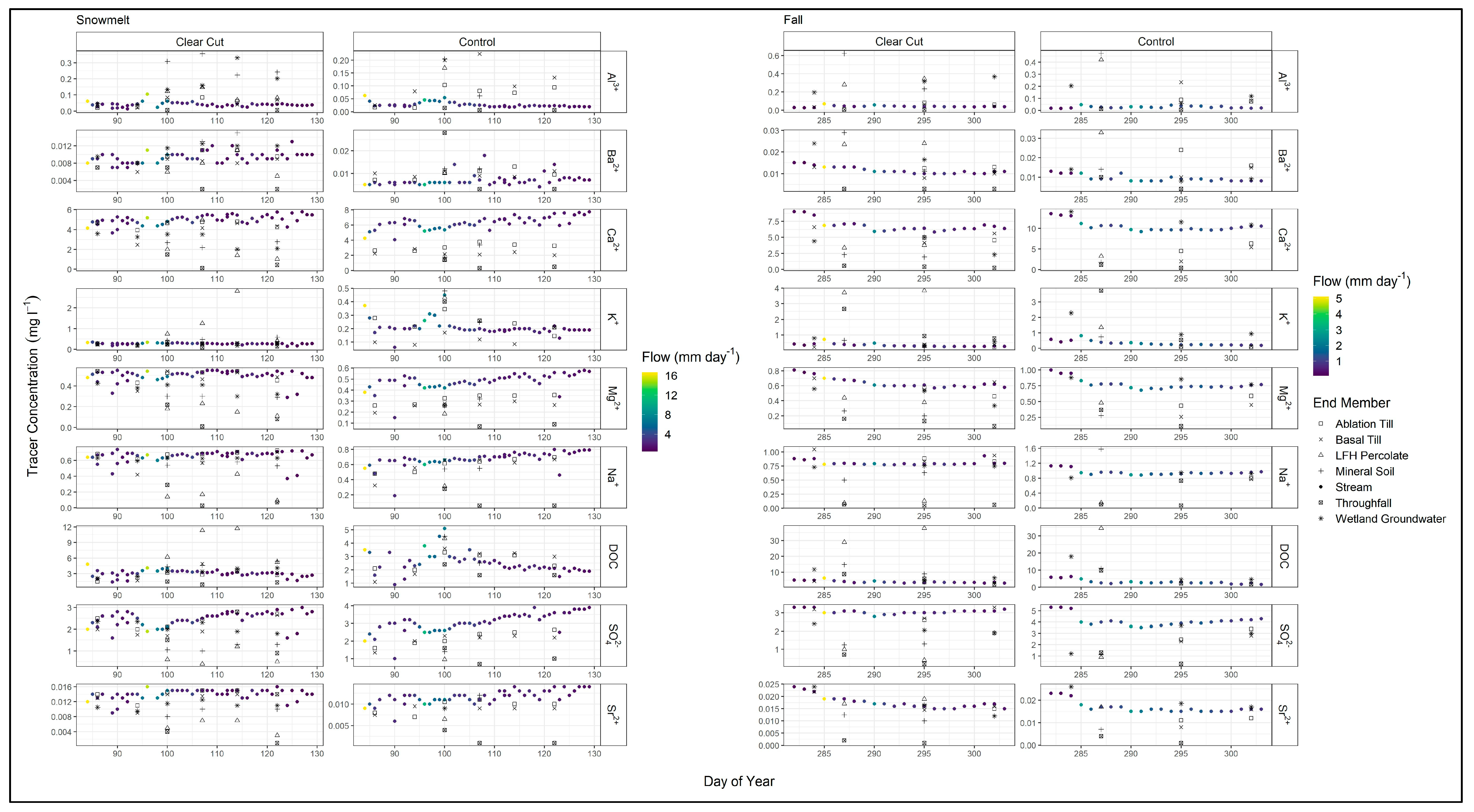
3.3. End Member and Stream Water Characterization

Solute concentrations ordered by throughfall, LFH percolate, wetland groundwater, mineral soil percolate, ablation till, basal till, and stream water (Figure 2) indicate that concentrations either increased or decreased sequentially from throughfall to the basal till groundwater end members. Generally, concentrations of Ca²⁺, Mg²⁺, Na⁻, SO₄²⁻, and Sr²⁺ were highest in the ablation and basal till groundwater end members and lowest in the throughfall and LFH percolate end members (Figure 2). Conversely, Al³⁺, K⁺, and DOC were elevated in the throughfall and LFH end members and lower in the ablation and basal till groundwater end members (Figure 2). One exception to the above patterns was Ba²⁺, which showed the highest concentrations in the wetland groundwater and mineral soil percolate end members and the lowest concentrations in the throughfall end member (Figure 2). There were few differences in these patterns between the clear-cut and control catchments and the snowmelt, summer, and fall flow conditions.

Tracer concentrations that were highest in the groundwater end members (Ca²⁺, Mg²⁺, Na⁻, SO₄²⁻, and Sr²⁺) increased throughout snowmelt in both the control and clear-cut catchments (Figure 4) while showing episodic decreases with increasing flow rates. During the fall wet-up, stream concentrations of Ca²⁺, Mg²⁺, Na⁻, SO₄²⁻, and Sr²⁺ decreased as flow increased and then showed no change as flow stabilized. During the summer storms, Ca²⁺, Mg²⁺, Na⁻, SO₄²⁻, and Sr²⁺ were inversely related to increasing stream flow (Figure 5). The opposite pattern was observed for Al³⁺, K⁺, and DOC, which were highest in the throughfall and LFH end members and increased with increasing flow during snowmelt, fall, and summer storms (Figure 4 and Figure 5). No pattern was observed for Ba²⁺ in stream water for any sampling period (Figure 4 and Figure 5).

3.4. EMMA Results

Stream water chemistry was not bounded by end members in the dataset (mixing subspace), and therefore, hydrograph separation was not possible. However, prominent end members contributing to the stream water mixture were identified based on their proximity to stream water values as described by Spencer et al. [63].

3.4.1. Snowmelt

During snowmelt, two principal components (PCs) explained 97.4%, 98.2%, and 95.5% of the variance for the clear-cut, control, and clear-cut wetland, respectively (Figure 6). The ablation and basal till groundwater end members were most like stream water chemistry for all three sampling locations, with the wetland end member being the next-closest for the clear-cut and clear-cut wetland. No wetland groundwater data were available in the control catchment during snowmelt. Throughfall and LFH percolate end members were most dissimilar from the stream water for all three end members. Higher flow rates in the clear-cut and control catchments trended towards the LFH percolate and mineral soil percolate end members. No obvious pattern was observed for increasing stream stage in the clear-cut wetland, and loadings trended away from the end members. Exceptions include K⁺ in the clear-cut and control trending towards the mineral soil and LFH percolate end members and DOC in the clear-cut wetland trending towards wetland groundwater, mineral soil, and LFH percolate in PC2.

3.4.2. Summer Storms

In the clear-cut, control, and clear-cut wetland, two PCs explained 97.8%, 96.6%, and 97.3% of the variance during storm 1 (Figure 7). Stream water values were closest to the ablation and basal till end members in the clear-cut, control, and clear-cut wetland. Additionally, the wetland groundwater and mineral soil water percolate were close to the stream water values in the control and mineral soil percolate in the clear-cut wetland. Increasing stream flow trended towards the wetland groundwater, throughfall, mineral soil, and LFH percolate in the clear-cut and clear-cut wetland. In the clear-cut catchment, Al³⁺ trended towards the wetland groundwater, mineral soil, and LFH percolate end member, while Mg²⁺ and Ca²⁺ trended towards the ablation and basal till end members. In the control catchment, Mg²⁺ and Ca²⁺ trended towards the wetland groundwater end member, while K⁺ trended towards the throughfall, mineral soil, and LFH percolate end members. For the clear-cut wetland, SO₄²⁻ trended towards the ablation till end member, while Mg²⁺ and Ca²⁺ trended towards the basal till end member.

For storm 4, two PCs explained 98.3%, 97.3%, and 98.2% of the variance in the clear-cut, control, and clear-cut wetland, respectively (Figure 7). Stream water chemistry was closest to the ablation and basal till end members in the clear-cut and clear-cut wetland, while wetland groundwater and ablation till end members were closest in the control. Increasing stream flow trended towards the mineral soil and LFH percolate in the clear-cut and towards all end members in the control. DOC trended towards the mineral soil and LFH percolate in the clear-cut, while all loadings trended away from end members in the control. DOC and Al³⁺ trended towards the wetland groundwater and LFH percolate in the clear-cut wetland.

3.4.3. Fall

Two PCs explained 99.1%, 99.4%, and 99.2% of the variance in the clear-cut, control, and clear-cut wetland, respectively (Figure 6). The ablation and basal till groundwater end members were closest to the stream water values at the clear-cut weir and clear-cut wetland, while the mineral soil percolate end member was closest to the stream water values in the control catchment. Higher flow rates trended towards the LFH percolate and wetland groundwater in the clear-cut and control catchments, respectively. Most loadings trended away from the end members. Exceptions include K⁺ moving towards wetland groundwater in the control and SO₄²⁻ towards all end members in PC1 for the clear-cut wetland.

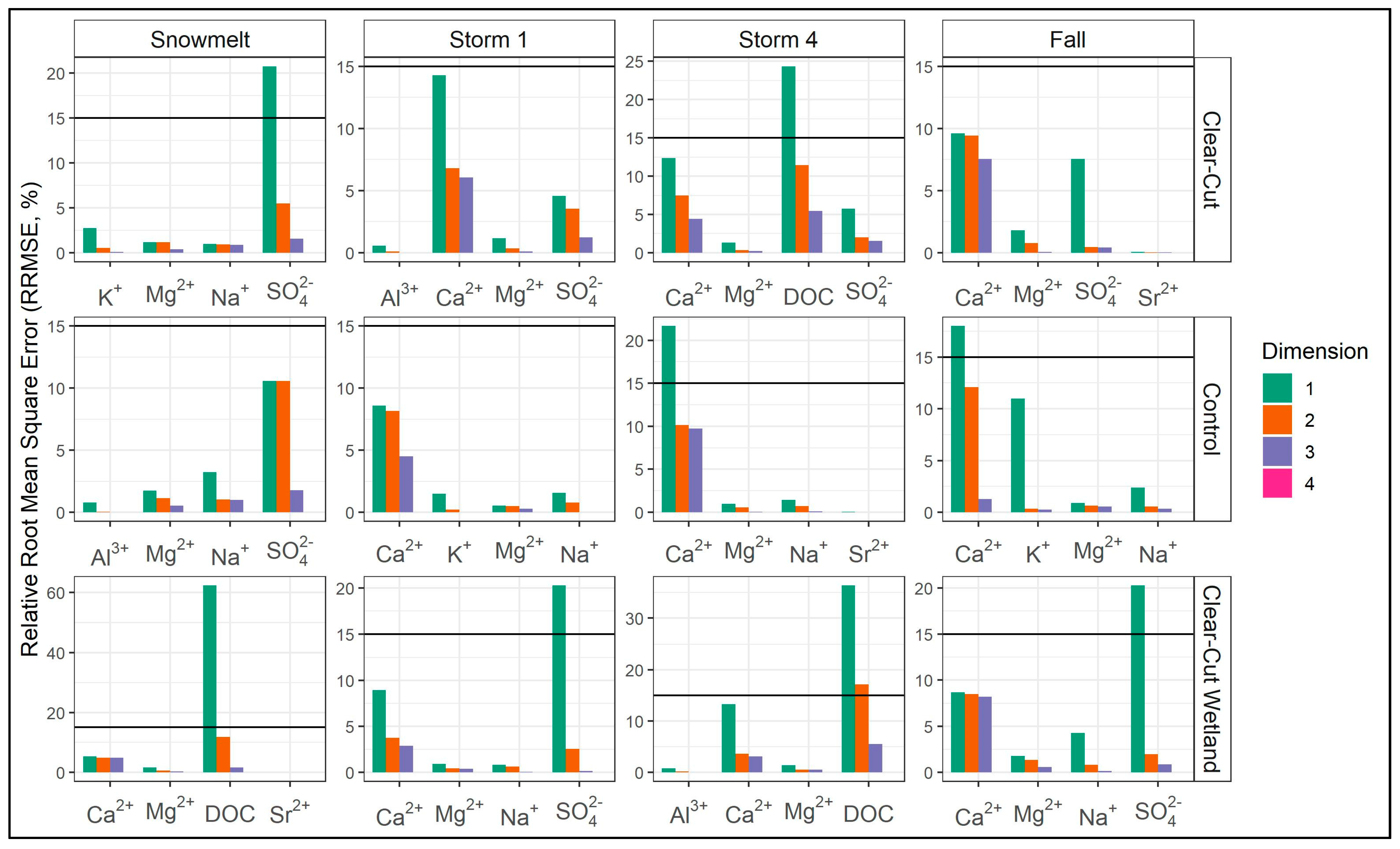
3.4.4. Residuals Analysis

Residuals analysis (RRMSE < 15%) confirmed that a two-dimensional mixing space was sufficient to explain the stream water chemistry for most sample locations for a range of flow conditions (Figure 8). Exceptions included the clear-cut wetland during storm 4, as DOC was above the 15% cut-off in the EMMA model (Figure 8). If stream water chemistry was properly bound by the end members, then a three-dimensional mixing space (four end members) would be required to explain the stream water chemistry in the clear-cut wetland during storm 4.

4. Discussion

4.1. Validity of EMMA at TLW

Three end members are required to explain stream water chemistry in the catchments (Figure 8) [50], and the data provided herein are comparable to other studies [48,52]. However, hydrograph separation in the present study was not completed because the stream water was not bound by end members within the mixing subspace. The only scenario where hydrograph separation could have been calculated was for the clear-cut wetland and the control catchment during storm 1 (Figure 7). However, this analysis still provides key insight into hydrologic processes that control runoff generation within these catchments and forms the conceptual framework to explain changes in stream chemistry. Studies have reported that while end members were not bound by stream water chemistry, they were previously used to infer runoff-generating processes in the Rocky Mountains of Alberta [63] and Canadian Shield of Quebec [48]. The lack of bounding of stream water by end member tracer concentrations could be caused by a missing end member that contributes to stream water [48,63]. Figure 2 and Figure 4 show that concentrations of Ca²⁺, Mg²⁺, Na⁻, SO₄²⁻, and Sr²⁺ within stream water lay outside the range observed in all the end members, which suggests that another end member is missing from this analysis. Missing end members could include a deeper groundwater source or a specific hillslope position that contribute to preferential inflows, which was not sampled in this study. Ali et al. [48] discussed the important role that aspect and specific hillslope positions, such as gullies, played in contributing to stream flow in the hardwood forests of the Hermine catchment at the Station de Biologie des Laurentides, Quebec, Canada, a study area having similar climate, geology, soils, and vegetation to the TLW. Additionally, specific hillslope positions or preferential inflows have been shown to influence stream water quality parameters such as DOC [68] and temperature [69]. Notably, the sampling design employed in this study may have precluded measurement of the complete range of water quality parameters for soil water and preferential surface flow pathways that contribute end members to stream flow.

It has been suggested that EMMA is not appropriate for hydrograph separation because spatial and temporal variation in solute end member chemistry with changing antecedent moisture conditions violates the assumptions of this procedure [70]. In the present study, end member chemistry was split by season to minimize these changes; however, the variability in solute chemistry (Figure 6 and Figure 7) and shifting median end member solute concentrations (Figure 4) suggest these assumptions were invalidated [48,70]. Accordingly, this provides further support that hydrograph separation using the mass balance equations should be avoided. Notably, this observation combined with the labor-intensive sampling regime required for EMMA may lead to the perception that it is not a cost-effective method for discerning hydrologic processes. However, using the proximity of end members to stream water chemistry within the mixing subspace (Figure 6 and Figure 7) and the hydro-chemical response of stream water (Figure 4 and Figure 5), inferences on hillslope channel connectivity and runoff-generation processes were still obtained. Additionally, this study highlights the importance of utilizing appropriate and thus different EMMA models (i.e., different tracers or end members) to represent different hydrologic scenarios, as shown by Ali et al. [48].

4.2. Insights into Hydrologic Processes

Ablation and basal till groundwater chemistries were the end members most similar to stream water in the mixing subspace, highlighting their role as primary sources contributing to stream water. This pattern was consistent across all three sampling locations with few seasonal differences (Figure 6 and Figure 7). This agrees with previous work at TLW, which showed that during snowmelt, a perched water table over the basal till routed water through the ablation till before reaching the stream channel [42,43]. Stream water chemistry at high flows trended towards the wetland groundwater, mineral soil water, and LFH percolate (Figure 6 and Figure 7), suggesting that the upper portions of the soil profile are only hydrologically connected during higher-flow conditions. Figure 4 supports this, with Al³⁺, K⁺, and DOC concentrations, which are highest in the LFH percolate, mineral soil water, and wetland groundwater end members, peaking in stream water at higher flows. Similar studies have shown that groundwater is often the dominant contributing end member to stream water in forested headwater catchments [52,53,65], and only under higher-flow conditions do the upper parts of the soil profile and hillslope become hydrologically connected [48,71].

Few seasonal differences in end member contributions to stream flow were observed and were rarely consistent among the three sampling locations. Exceptions were observed with the wetland groundwater and mineral soil percolate end members being closest to stream water values for the control catchment during the fall and summer storms (Figure 6 and Figure 7). The lower contributions from the ablation and basal till may be due to the lack of data from these end members in the control catchment during summer. Given that few groundwater samples were collected during storm events, and a stream response to storms was still observed, it could be hypothesized that these end members were not major contributors to stream water, as there was rarely enough ground water to collect a sample. The location of the piezometers may have also missed critical subsurface flow paths such as those described by Ali et al. [48]. Additionally, the proximity of the wetland to the catchment outlet explains the prominent contributions of wetland groundwater to stream flow in the control catchment.

4.3. Wetland Contributions to Stream Flow

While groundwater contributions were the primary source of water within the clear-cut and control catchments, wetland groundwater contributions were an important secondary source, especially during summer storms (Figure 6 and Figure 7). This is especially apparent in the control catchment, where the wetland is directly upstream of the catchment outlet. During the summer storms, wetland groundwater solute chemistry was closest to stream water in the mixing subspace in the control catchment, while the groundwater end members were closest in the clear-cut (Figure 7). The wetland signal within the clear-cut may be diluted by hillslope contributions, as the wetland is near the stream-initiation point, unlike its location directly above the catchment outlet in the control. Further support for this hypothesis is the number of zero-flow days observed in these catchments. Flow was sustained in the control catchment during the summer (no zero-flow days), while the clear-cut had 48 zero-flow days (Table 2). While these differences may be caused by the impacts of legacy harvesting, they are more likely the result of differences in wetland position between the two study catchments. Studies have shown that small wetlands can act as sponges that fill up during wet periods and slowly drain, sustaining flow during dry periods [24,72]. Work exploring the effect of wetland cover on mean water-travel times supports this theory, as the relationship between travel times and wetland cover is dependent on the antecedent moisture conditions [23,73]. During wet time periods, wetlands rapidly transport water laterally through the upper parts of the soil profile due to low water-storage capacity and high hydraulic conductivities [23]. During dry periods, wetlands may act as a small reservoir collecting water from surrounding hillslopes and slowly draining into the stream channel [23,73]. Notably, in the present study, stream flow within the control catchment was mostly sourced by wetland groundwater. The proximity of the wetland to the control catchment outlet maintained flow throughout the summer.

4.4. Legacy Harvesting Effects on End Member Contributions to Stream Flow

Despite the differences in wetland groundwater contributions to stream flow between the control and clear-cut catchments, there are few differences between the clear-cut and control catchments, suggesting legacy forest harvesting has limited impact on the prominent end member contributions to stream flow. Previous work at TLW found that forest harvesting increased the proportion of water moving through the upper parts of the soil profile based on K:SiO₂ molar ratios four years after harvesting [38]. If harvesting was still impacting these flow paths, it would be expected that the clear-cut mineral soil and LFH percolate end member contributions to stream water would be larger than in the control. As no differences were observed in end member contributions to stream flow between the control and clear-cut catchments, it can be assumed that the harvesting-induced flow path changes have recovered. As signs of flow path recovery have been observed 15 years after harvesting [10], it is reasonable to assume a complete recovery may have occurred by the time of this study. This suggests that forest harvesting may be a suitable source-water-protection strategy for this landscape, as there are limited long-term harvesting impacts on runoff-generation processes that most affect stream water quality. However, recent work conducted at TLW has shown how harvesting impacts on water yield in an adjacent catchment that was subject to a selection harvest treatment may have persisted until 2020 [10,74]. This in combination with the high variability observed in end member concentrations suggests the results from this study should be interpreted cautiously. However, the lack of change in end member contributions to stream flow does not necessarily mean there would be no change in stream water yield. Future work should continue to explore the impacts of forest harvesting on these runoff-generation processes to further inform the impacts on both water quantity and quality.

4.5. Implications for Water Quality and Treatability

Previous work has provided insights to the behavior of numerous water quality parameters and their response to harvesting at TLW [13,61]. Solutes such as K⁺ and DOC were still elevated in the study catchments 21 years after harvesting; these responses were attributed to long-term changes in solute demand/availability and hillslope channel connectivity [13]. As both solutes are generally associated with shallow flow paths, it follows that mineral soil and LFH end members may contribute more to stream flow in harvested catchments. However, the results from EMMA did not support this hypothesis and may suggest that changes in solute availability on the landscape are driving the observed harvesting response. This shows the importance of quantifying not only hillslope channel connectivity but also nutrient and solute availability when evaluating the suitability of landscape management decisions such as forest harvesting as source-water-protection strategies.

Previous studies have identified wetlands as a critical source of numerous water quality parameters at TLW [23,60,75]. Solutes such as DOC, dissolved organic nitrogen (DON), total phosphorus (TP), and total dissolved phosphorus (TDP) were all elevated in catchments with large wetland fractions at TLW [60,75]. The unique biogeochemical processes occurring in these wetlands heavily influence the solubility, lability, and mobility of these nutrients [60,75]. The results from this study clearly show the important influence wetlands play in runoff generation within these headwater catchments, providing further evidence of their influence on both water quantity and quality. Wetlands appear to have a disproportionately larger influence on stream water quantity and quality relative to other landscape features such as hillslopes. Therefore, special care should be taken by land managers to ensure wetlands protection given their sensitivity to landscape disturbance [24].

5. Conclusions

End member mixing analysis was used to evaluate the dominant sources of hillslope runoff that contribute to the generation of stream flow in a legacy clear-cut and control catchment at TLW. Tracer concentrations either increased (Ca²⁺, Mg²⁺, Na⁻, SO₄²⁻, and Sr²⁺) or decreased (Al³⁺, K⁺, and DOC) sequentially from throughfall to the basal till groundwater end members. Stream water was not bounded by end members in the mixing subspace, making hydrograph separation impossible using this dataset. Despite this limitation, results suggest that ablation and basal till groundwater end members were the major contributors to stream flow in both the legacy clear-cut and control catchments during snowmelt and fall. Groundwater originating from wetlands within the stream network was also identified as a prominent source of stream flow in both catchments. During the summer storms, wetland groundwater was the dominant source of stream flow to the control catchment. However, wetland position in the landscape and the degree of hydrologic connectivity to the stream channel influenced the contributions of wetland groundwater to stream flow. There were few differences between end member contributions to stream flow in the legacy clear-cut and control catchments suggesting hydrologic recovery had largely occurred 24 years post harvesting. Future studies should focus on identifying critical hillslope positions or preferential inflows that likely represent large contributions to stream flow within these catchments. Identifying these critical positions may increase the chances of hydrograph separation using EMMA and provide more quantitative insight into the impacts of changing antecedent moisture conditions and landscape disturbances on runoff-generation processes. Overall, the results from this study suggest that legacy forest harvesting has a relatively small impact on hydrological processes. Accordingly, forest harvesting may be a suitable source-water-protection strategy for Canadian Shield catchments. Additionally, this study demonstrates the utility of EMMA to evaluate key drivers that influence the relationship between hydrologic processes and water quality. Such information is critical for land managers and drinking water providers to develop and evaluate source-water-protection strategies and drinking-water safety plans and inform landscape management decisions.

References

1. Emelko, M.B.; Silins, U.; Bladon, K.D.; Stone, M. Implications of Land Disturbance on Drinking Water Treatability in a Changing Climate: Demonstrating the Need for “Source Water Supply and Protection” Strategies. Water Res. 2011, 45, 461–472. [Google Scholar] [CrossRef] [PubMed]
2. MacDonald, R.; Shemie, D. Urban Water Blueprint; The Nature Conservancy: Washington, DC, USA, 2014. [Google Scholar]
3. Stein, S.; Butler, B. On the Front Line: Private Forests & Water Resources; US Department of Agriculture, Forest Service: Washington, DC, USA, 2004; Volume FS-790.
4. Stein, S.M.; McRoberts, R.E.; Alig, R.J.; Nelson, M.D.; Theobald, D.M.; Eley, M.; Dechter, M.; Carr, M. Forests on the Edge: Housing Development on America’s Private Forests; US Department of Agriculture, Forest Service, Pacific Northwest Research Station: Washington, DC, USA, 2005.
5. Sun, G.; Vose, J.M. Forest Management Challenges for Sustaining Water Resources in the Anthropocene. Forests 2016, 7, 68. [Google Scholar] [CrossRef] [Green Version]
6. de Groot, R.; Brander, L.; van der Ploeg, S.; Costanza, R.; Bernard, F.; Braat, L.; Christie, M.; Crossman, N.; Ghermandi, A.; Hein, L.; et al. Global Estimates of the Value of Ecosystems and Their Services in Monetary Units. Ecosyst. Serv. 2012, 1, 50–61. [Google Scholar] [CrossRef]
7. Costanza, R.; d’Arge, R.; de Groot, R.; Farber, S.; Grasso, M.; Hannon, B.; Limburg, K.; Naeem, S.; O’Neill, R.V.; Paruelo, J.; et al. The Value of the World’s Ecosystem Services and Natural Capital. Ecol. Econ. 1998, 25, 3–15. [Google Scholar] [CrossRef]
8. Caretta, M.A.; Mukherji, A.; Arfanuzzaman, M.; Betts, R.A.; Gelfan, A.; Hirabayashi, Y.; Lissner, T.K.; Liu, J.; Gunn, E.L.; Morgan, R.; et al. Water. In Climate Change 2022: Impacts, Adaptation, and Vulnerability. Contribution of Working Group II to the Sixth Assessment Report of the Intergovernmental Panel on Climate Change; Pörtner, H.-O., Roberts, D.C., Tignor, M., Poloczanska, E.S., Mintenbeck, K., Alegría, A., Craig, M., Langsdorf, S., Löschke, S., Möller, V., et al., Eds.; Cambridge University Press: Cambridge, UK; New York, NY, USA, 2022; pp. 551–712. ISBN 9781009325844. [Google Scholar]
9. Smith, H.G.; Sheridan, G.J.; Nyman, P. Wildfire Effects on Water Quality in Forest Catchments: A Review with Implications for Water Supply. J. Hydrol. 2011, 396, 170–192. [Google Scholar] [CrossRef]
10. Buttle, J.M.; Beall, F.D.; Webster, K.L.; Hazlett, P.W.; Creed, I.F.; Semkin, R.G.; Jeffries, D.S. Hydrologic Response to and Recovery from Differing Silvicultural Systems in a Deciduous Forest Landscape with Seasonal Snow Cover. J. Hydrol. 2018, 557, 805–825. [Google Scholar] [CrossRef]
11. Jones, J.A. Hydrologic Processes and Peak Discharge Response to Forest Removal, Regrowth, and Roads in 10 Small, Experimental Basins, Western Cascades, Oregon. Water Resour. Res. 2000, 36, 2621–2642. [Google Scholar] [CrossRef] [Green Version]
12. Neary, D.G.; Ice, G.G.; Jackson, C.R. Linkages between Forest Soils and Water Quality and Quantity. For. Ecol. Manage. 2009, 258, 2269–2281. [Google Scholar] [CrossRef]
13. Webster, K.L.; Leach, J.A.; Hazlett, P.W.; Buttle, J.M.; Emilson, E.J.; Creed, I. Long Term Stream Chemistry Response to Harvesting in a Northern Hardwood Forest Watershed Experiencing Environmental Change. For. Ecol. Manag. 2022, 519, 120345. [Google Scholar] [CrossRef]
14. Silins, U.; Stone, M.; Emelko, M.B.; Bladon, K.D. Catena Sediment Production Following Severe Wildfire and Post-Fire Salvage Logging in the Rocky Mountain Headwaters of the Oldman River Basin, Alberta. Catena 2009, 79, 189–197. [Google Scholar] [CrossRef]
15. Emelko, M.B.; Stone, M.; Silins, U.; Allin, D.; Collins, A.L.; Williams, C.H.S.; Martens, A.M.; Bladon, K.D. Sediment-Phosphorus Dynamics Can Shift Aquatic Ecology and Cause Downstream Legacy Effects after Wildfire in Large River Systems. Glob. Chang. Biol. 2016, 22, 1168–1184. [Google Scholar] [CrossRef] [PubMed]
16. Stone, M.; Collins, A.L.; Silins, U.; Emelko, M.B.; Zhang, Y.S. The Use of Composite Fingerprints to Quantify Sediment Sources in a Wildfire Impacted Landscape, Alberta, Canada. Sci. Total Environ. 2014, 473–474, 642–650. [Google Scholar] [CrossRef]
17. Stone, M.; Krishnappan, B.G.; Silins, U.; Emelko, M.B.; Williams, C.H.S.; Collins, A.L.; Spencer, S.A. A New Framework for Modelling Fine Sediment Transport in Rivers Includes Flocculation to Inform Reservoir Management in Wildfire Impacted Watersheds. Water 2021, 13, 2319. [Google Scholar] [CrossRef]
18. Buttle, J.M. The Effects of Forest Harvesting on Forest Hydrology and Biogeochemistry. In Forest Hydrology and Biogeochemistry: Synthesis of Past Research and Future Directions; Springer Science & Business Media: Berlin/Heidelberg, Germany, 2011; pp. 659–677. ISBN 978-94-007-1362-8. [Google Scholar]
19. Jones, J.A.; Creed, I.F.; Hatcher, K.L.; Warren, R.J.; Adams, M.B.; Benson, M.H.; Boose, E.; Brown, W.A.; Campbell, J.L.; Covich, A.; et al. Ecosystem Processes and Human Influences Regulate Streamflow Response to Climate Change at Long-Term Ecological Research Sites. Bioscience 2012, 62, 390–404. [Google Scholar] [CrossRef] [Green Version]
20. Creed, I.F.; Jones, J.A.; Archer, E.; Claassen, M.; Ellison, D.; McNulty, S.G.; van Noordwijk, M.; Vira, B.; Wei, X.; Bishop, K.; et al. Managing Forests for Both Downstream and Downwind Water. Front. For. Glob. Chang. 2019, 2, 64. [Google Scholar] [CrossRef] [Green Version]
21. Zhang, M.; Wei, X.; Li, Q. Do the Hydrological Responses to Forest Disturbances in Large Watersheds Vary along Climatic Gradients in the Interior of British Columbia, Canada? Ecohydrology 2017, 10, e1840. [Google Scholar] [CrossRef]
22. McDonnell, J.J.; Evaristo, J.; Bladon, K.D.; Buttle, J.; Creed, I.F.; Dymond, S.F.; Grant, G.; Iroume, A.; Jackson, C.R.; Jones, J.A.; et al. Water Sustainability and Watershed Storage. Nat. Sustain. 2018, 1, 378–379. [Google Scholar] [CrossRef]
23. Leach, J.A.; Buttle, J.M.; Webster, K.L.; Hazlett, P.W.; Jeffries, D.S. Travel Times for Snowmelt-Dominated Headwater Catchments: Influences of Wetlands and Forest Harvesting, and Linkages to Stream Water Quality. Hydrol. Process. 2020, 34, 2154–2175. [Google Scholar] [CrossRef]
24. Webster, K.L.; Beall, F.D.; Creed, I.F.; Kreutzweiser, D.P. Impacts and Prognosis of Natural Resource Development on Water and Wetlands in Canada’s Boreal Zone. Environ. Rev. 2015, 23, 78–131. [Google Scholar] [CrossRef] [Green Version]
25. Blackburn, E.A.J.; Emelko, M.B.; Dickson-Anderson, S.; Stone, M. Advancing on the Promises of Techno-Ecological Nature-Based Solutions: A Framework for Green Technology in Water Supply and Treatment. Blue-Green Syst. 2021, 3, 81–94. [Google Scholar] [CrossRef]
26. Emelko, M.; Ho Sham, C. Wildfire Impacts on Water Supplies and the Potential for Mitigation, Web Report #4529; Water Research Foundation: Denver, CO, USA; Canadian Water Network: Waterloo, ON, Canada, 2014. [Google Scholar]
27. Mackay, D.S.; Band, L.E. Forest Ecosystem Processes at the Watershed Scale: Dynamic Coupling of Distributed Hydrology and Canopy Growth. Hydrol. Process. 1997, 11, 1197–1217. [Google Scholar] [CrossRef]
28. Murray, C.D.; Buttle, J.M. Impacts of Clearcut Harvesting on Snow Accumulation and Melt in a Northern Hardwood Forest. J. Hydrol. 2003, 271, 197–212. [Google Scholar] [CrossRef]
29. Chanasyk, D.S.; Whitson, I.R.; Mapfumo, E.; Burke, J.M.; Prepas, E.E. The Impacts of Forest Harvest and Wildfire on Soils and Hydrology in Temperate Forests: A Baseline to Develop Hypotheses for the Boreal Plain. J. Environ. Eng. Sci. 2003, 2, S51–S62. [Google Scholar] [CrossRef]
30. Startsev, A.D.; McNabb, D.H. Effects of Skidding on Forest Soil Infiltration in West-Central Alberta. Can. J. Soil Sci. 2000, 80, 617–624. [Google Scholar] [CrossRef]
31. Whitson, I.R.; Chanasyk, D.S.; Prepas, E.E. Hydraulic Properties of Orthic Gray Luvisolic Soils and Impact of Winter Logging. J. Environ. Eng. Sci. 2003, 2, S41–S49. [Google Scholar] [CrossRef]
32. Williamson, J.R.; Neilsen, W.A. The Influence of Forest Site on Rate and Extent of Soil Compaction and Profile Disturbance of Skid Trails during Ground-Based Harvesting. Can. J. Fish. Aquat. Sci. 2000, 30, 1196–1205. [Google Scholar] [CrossRef]
33. Johnson, A.C.; Edwards, R.T.; Erhardt, R. Ground-Water Response to Forest Harvest: Implicaitons for Hillslope Stability. J. Am. Water Resour. Assoc. 2007, 43, 134–147. [Google Scholar] [CrossRef]
34. Murray, C.D.; Buttle, J.M. Infiltration and Soil Water Mixing on Forested and Harvested Slopes during Spring Snowmelt, Turkey Lakes Watershed, Central Ontario. J. Hydrol. 2005, 306, 1–20. [Google Scholar] [CrossRef]
35. Nijzink, R.; Hutton, C.; Pechlivanidis, I.; Capell, R.; Arheimer, B.; Freer, J.; Han, D. The Evolution of Root-Zone Moisture Capacities after Deforestation: A Step towards Hydrological Predictions under Change? Hydrol. Earth Syst. Sci. 2016, 20, 4775–4799. [Google Scholar] [CrossRef] [Green Version]
36. Buttle, J.M.; Webster, K.L.; Hazlett, P.W.; Jeffries, D.S. Quickflow Response to Forest Harvesting and Recovery in a Northern Hardwood Forest Landscape. Hydrol. Process. 2019, 33, 47–65. [Google Scholar] [CrossRef] [Green Version]
37. Monteith, S.S.; Buttle, J.M.; Hazlett, P.W.; Beall, F.D.; Semkin, R.G.; Jeffries, D.S. Paired-Basin Comparison of Hydrological Response in Harvested and Undisturbed Hardwood Forests during Snowmelt in Central Ontario: I. Streamflow, Groundwater and Flowpath Behaviour. Hydrol. Process. 2006, 20, 1095–1116. [Google Scholar] [CrossRef]
38. Monteith, S.S.; Buttle, J.M.; Hazlett, P.W.; Beall, F.D.; Semkin, R.G.; Jeffries, D.S. Paired-Basin Comparison of Hydrologic Response in Harvested and Undisturbed Hardwood Forests during Snowmelt in Central Ontario: II. Streamflow Sources and Groundwater Residence Times. Hydrol. Process. 2006, 20, 1117–1136. [Google Scholar] [CrossRef]
39. Sørensen, R.; Ring, E.; Meili, M.; Högbom, L.; Seibert, J.; Grabs, T.; Laudon, H.; Bishop, K. Forest Harvest Increases Runoff Most during Low Flows in Two Boreal Streams. AMBIO 2009, 38, 357–363. [Google Scholar] [CrossRef]
40. Bosch, J.M.; Hewlett, J.D. A Review of Catchment Experiments to Determine the Effect of Vegetation Changes on Water Yield and Evapotranspiration. J. Hydrol. 1982, 55, 3–23. [Google Scholar] [CrossRef]
41. Webster, K.L.; Leach, J.A.; Hazlett, P.W.; Fleming, R.L.; Emilson, E.J.S.; Houle, D.; Chan, K.H.Y.; Norouzian, F.; Cole, A.S.; O’Brien, J.M.; et al. Turkey Lakes Watershed, Ontario, Canada: 40 Years of Interdisciplinary Whole-Ecosystem Research. Hydrol. Process. 2021, 35, e14109. [Google Scholar] [CrossRef]
42. Hazlett, P.W.; Semkin, R.G.; Beall, F.D. Hydrologic Pathways during Snowmelt in First-Order Stream Basins at the Turkey Lakes Watershed. Ecosystems 2001, 4, 527–535. [Google Scholar] [CrossRef]
43. Semkin, R.G.; Hazlett, P.W.; Beall, F.D.; Jeffries, D.S. Development of Stream Water Chemistry during Spring Melt in a Northern Hardwood Forest. Water Air Soil Pollut. Focus 2002, 2, 37–61. [Google Scholar] [CrossRef]
44. Swank, W.T.; Vose, J.M.; Elliott, K.J. Long-Term Hydrologic and Water Quality Responses Following Commercial Clearcutting of Mixed Hardwoods on a Southern Appalachian Catchment. For. Ecol. Manag. 2001, 143, 163–178. [Google Scholar] [CrossRef]
45. Christophersen, N.; Neal, C.; Hooper, R.P.; Vogt, R.D.; Andersen, S. Modelling Streamwater Chemistry as a Mixture of Soilwater End-Members—A Step towards Second-Generation Acidification Models. J. Hydrol. 1990, 116, 307–320. [Google Scholar] [CrossRef]
46. Christophersen, N.; Hooper, R. Multivariate Analysis of Stream Water Chemical Data: The Use of Principal Components Analysis for the End-Member Mixing Problem. Water Resour. Res. 1992, 28, 99–107. [Google Scholar] [CrossRef]
47. James, A.L.; Roulet, N.T. Investigating the Applicability of End-Member Mixing Analysis (EMMA) across Scale: A Study of Eight Small, Nested Catchments in a Temperate Forested Watershed. Water Resour. Res. 2006, 42, 1–17. [Google Scholar] [CrossRef] [Green Version]
48. Ali, G.A.; Roy, A.G.; Turmel, M.C.; Courchesne, F. Source-to-Stream Connectivity Assessment through End-Member Mixing Analysis. J. Hydrol. 2010, 392, 119–135. [Google Scholar] [CrossRef]
49. Hooper, R.P. Applying the Scientific Method to Small Catchment Studies: A Review of the Panola Mountain Experience. Hydrol. Process. 2001, 15, 2039–2050. [Google Scholar] [CrossRef]
50. Hooper, R.P. Diagnostic Tools for Mixing Models of Stream Water Chemistry. Water Resour. Res. 2003, 39, 1–13. [Google Scholar] [CrossRef]
51. Inamdar, S. The Use of Geochemical Mixing Models to Derive Runoff Sources and Hydrologic Flow Paths. In Forest Hydrology and Biogeochemistry: Synthesis of Past Research and Future Directions; Springer Science & Business Media: Berlin/Heidelberg, Germany, 2011; Volume 216, pp. 163–183. ISBN 978-94-007-1362-8. [Google Scholar]
52. Katsuyama, M.; Ohte, N.; Kobashi, S. A Three-Component End-Member Analysis of Streamwater Hydrochemistry in a Small Japanese Forested Headwater Catchment. Hydrol. Process. 2001, 15, 249–260. [Google Scholar] [CrossRef]
53. Burns, D.A.; Mcdonnell, J.J.; Hooper, R.P.; Peters, N.E.; Freer, J.E.; Kendall, C.; Beven, K. Quantifying Contributions to Storm Runoff through End-Member Mixing Analysis and Hydrologic Measurements at the Panola Mountain Research Watershed (Georgia, USA). Hydrol. Process. 2001, 15, 1903–1924. [Google Scholar] [CrossRef]
54. Wellington, B.I.; Driscoll, C.T. The Episodic Acidification of a Stream with Elevated Concentrations of Dissolved Organic Carbon. Hydrol. Process. 2004, 18, 2663–2680. [Google Scholar] [CrossRef]
55. van Verseveld, W.J.; McDonnell, J.J.; Lajtha, K. A Mechanistic Assessment of Nutrient Flushing at the Catchment Scale. J. Hydrol. 2008, 358, 268–287. [Google Scholar] [CrossRef]
56. Jeffries, D.S.; Kelso, J.R.M.; Morrison, I.K. Physical, Chemical, and Biological Characteristics of the Turkey Lakes Watershed, Central Ontario, Canada. Can. J. Fish. Aquat. Sci. 1988, 45, 3–13. [Google Scholar] [CrossRef]
57. Hazlett, P.W.; Foster, N.W. Topographic Controls of Nitrogen, Sulfur, and Carbon Transport From a Tolerant Hardwood Hillslope. Water Air Soil Pollut. Focus 2002, 2, 63–80. [Google Scholar] [CrossRef]
58. OMNRF. Forest Management Guide to Silviculture in the Great Lakes-St. Lawrence and Boreal Forests of Ontario; Queens Printer for Ontario: Toronto, ON, USA, 2015; ISBN 9781460650998.
59. Morrison, I.K.; Cameron, D.A.; Foster, N.W.; Groot, A. Forest Research at the Turkey Lakes Watershed. For. Chron. 1999, 75, 395–399. [Google Scholar] [CrossRef] [Green Version]
60. Creed, I.F.; Sanford, S.E.; Beall, F.D.; Molot, L.A.; Dillon, P.J. Cryptic Wetlands: Integrating Hidden Wetlands in Regression Models of the Export of Dissolved Organic Carbon from Forested Landscapes. Hydrol. Process. 2003, 17, 3629–3648. [Google Scholar] [CrossRef]
61. Webster, K.L.; Leach, J.A.; Houle, D.; Hazlett, P.W.; Emilson, E.J.S. Acidification Recovery in a Changing Climate: Observations from Thirty-Five Years of Stream Chemistry Monitoring in Forested Headwater Catchments at the Turkey Lakes Watershed, Ontario. Hydrol. Process. 2021, 35, e14346. [Google Scholar] [CrossRef]
62. Pulley, S.; Collins, A.L. Tracing Catchment Fine Sediment Sources Using the New SIFT (SedIment Fingerprinting Tool) Open Source Software. Sci. Total Environ. 2018, 635, 838–858. [Google Scholar] [CrossRef] [PubMed]
63. Spencer, S.A.; Anderson, A.E.; Silins, U.; Collins, A.L. Hillslope and Groundwater Contributions to Streamflow in a Rocky Mountain Watershed Underlain by Glacial till and Fractured Sedimentary Bedrock. Hydrol. Earth Syst. Sci. 2021, 25, 237–255. [Google Scholar] [CrossRef]
64. Pulley, S.; Foster, I.; Antunes, P. The Uncertainties Associated with Sediment Fingerprinting Suspended and Recently Deposited Fluvial Sediment in the Nene River Basin. Geomorphology 2015, 228, 303–319. [Google Scholar] [CrossRef] [Green Version]
65. Fuss, C.B.; Driscoll, C.T.; Green, M.B.; Groffman, P.M. Hydrologic Flowpaths during Snowmelt in Forested Headwater Catchments under Differing Winter Climatic and Soil Frost Regimes. Hydrol. Process. 2016, 30, 4617–4632. [Google Scholar] [CrossRef]
66. R Core Team. R: A Language and Environment for Statistical Computing. Available online: https://www.r-project.org/ (accessed on 1 September 2019).
67. Liu, F.; Bales, R.C.; Conklin, M.H.; Conrad, M.E. Streamflow Generation from Snowmelt in Semi-Arid, Seasonally Snow-Covered, Forested Catchments, Valles Caldera, New Mexico. Water Resour. Res. 2008, 44, 1–13. [Google Scholar] [CrossRef] [Green Version]
68. Ploum, S.W.; Leach, J.A.; Laudon, H.; Kuglerová, L. Groundwater, Soil, and Vegetation Interactions at Discrete Riparian Inflow Points (DRIPs) and Implications for Boreal Streams. Front. Water 2021, 3, 669007. [Google Scholar] [CrossRef]
69. Leach, J.A.; Lidberg, W.; Kuglerová, L.; Peralta-Tapia, A.; Ågren, A.; Laudon, H. Evaluating Topography-Based Predictions of Shallow Lateral Groundwater Discharge Zones for a Boreal Lake-Stream System. Water Resour. Res. 2017, 53, 5420–5437. [Google Scholar] [CrossRef]
70. Inamdar, S.; Dhillon, G.; Singh, S.; Dutta, S.; Levia, D.; Scott, D.; Mitchell, M.; Van Stan, J.; McHale, P. Temporal Variation in End-Member Chemistry and Its Influence on Runoff Mixing Patterns in a Forested, Piedmont Catchment. Water Resour. Res. 2013, 49, 1828–1844. [Google Scholar] [CrossRef] [Green Version]
71. Detty, J.M.; Mcguire, K.J. Topographic Controls on Shallow Groundwater Dynamics: Implications of Hydrologic Connectivity between Hillslopes and Riparian Zones in a till Mantled Catchment. Hydrol. Process. 2010, 24, 2222–2236. [Google Scholar] [CrossRef]
72. Wagener, T.; Sivapalan, M.; Troch, P.; Woods, R. Catchment Classification and Hydrologic Similarity. Geogr. Compass 2007, 1, 901–931. [Google Scholar] [CrossRef]
73. Lane, D.; McCarter, C.P.R.; Richardson, M.; McConnell, C.; Field, T.; Yao, H.; Arhonditsis, G.; Mitchell, C.P.J. Wetlands and Low-Gradient Topography Are Associated with Longer Hydrologic Transit Times in Precambrian Shield Headwater Catchments. Hydrol. Process. 2020, 34, 598–614. [Google Scholar] [CrossRef]
74. Leach, J.A.; Hudson, D.T.; Moore, R.D. Assessing Stream Temperature Response and Recovery for Different Harvesting Systems in Northern Hardwood Forests Using 40 Years of Spot Measurements. Hydrol. Process. 2022, 36, e14753. [Google Scholar] [CrossRef]
75. Mengistu, S.G.; Creed, I.F.; Webster, K.L.; Enanga, E.; Beall, F.D. Searching for Similarity in Topographic Controls on Carbon, Nitrogen and Phosphorus Export from Forested Headwater Catchments. Hydrol. Process. 2014, 28, 3201–3216. [Google Scholar] [CrossRef]
Figure 1. Maps of Turkey Lakes Watershed (left) and sub catchments C31 (clear-cut; top right) and C32 (control; bottom right). Locations of stream water sampling sites, groundwater piezometers, soil pits, throughfall collectors, and wetlands are marked.
Water 15 02825 g001
Figure 2. Boxplots of tracer concentrations for each end member and stream chemistry in the clear-cut (C31) and control (C32) catchments during the snowmelt, summer, and fall sampling periods. Results from the Kruskal–Wallis H-test are shown above (* p ≤ 0.05, ** p ≤ 0.01, *** p ≤ 0.001, and **** p ≤ 0.0001).
Water 15 02825 g002
Figure 3. Example bivariate plot from the clear-cut catchment (C31) during snowmelt. Top right of the plot represents the Pearson’s correlation coefficient and level of significance (* p ≤ 0.05, ** p ≤ 0.01, and *** p ≤ 0.001) for the linear relationships between each tracer. Red line shows the line of best fit using linear regression.
Water 15 02825 g003
Figure 4. Time series of median end member and stream water tracer concentrations (mg L−1) on the day of sampling for the snowmelt and fall sampling periods. Color represents daily stream flow (mm day−1), and symbols represent the different end members.
Water 15 02825 g004
Figure 5. Hydrograph (black line) and tracer (blue dots) response of stream water during the two summer storms. Stream flow is in L s−1 ha−1, and tracer concentrations are in mg L−1.
Water 15 02825 g005
Figure 6. EMMA models for the clear-cut, control, and clear-cut wetland sampling locations during the snowmelt and fall sampling periods using the first two principal components that explain stream water chemistry. Grey circles show stream water points, with circle size denoting either stream flow (mm) for the clear-cut and control catchment or head (cm) for the clear-cut wetland. Colored points and error bars denote the median ± median absolute deviation (MAD) end member tracer concentrations that were projected into the mixing subspace defined by the stream water chemistry. Arrows denote the loadings from the principal component analysis (PCA) for each tracer used in the EMMA model.
Water 15 02825 g006
Figure 7. EMMA models for the clear-cut, control, and clear-cut wetland sampling locations during storm 1 and storm 4 using the first two principal components that explain the most variation in stream water chemistry. Grey circles show stream water points, with circle size denoting either stream flow (L s−1 ha−1) for the clear-cut and control catchment or head (cm) for the clear-cut wetland. Colored points and error bars denote the median ± MAD end member tracer concentrations that were projected into the mixing subspace defined by the stream water chemistry. Arrows denote the loadings from the principal component analysis (PCA) for each tracer used in the EMMA model.
Water 15 02825 g007
Figure 8. Relative root-mean-square error (RRMSE, %) for the tracers used in the EMMA models. Horizontal line represents the 15% cut-off threshold recommended by James and Roulet [47]. Color represents the RRMSE explained by each principal component or dimension of the mixing subspace.
Water 15 02825 g008